Interferometry using spinor Bose-Einstein condensates

Abstract

We study the time-evolution of an optically trapped spinor Bose-Einstein condensate under the influence of a dominating magnetic bias field in the $z$-direction, and a perpendicular smaller field that couples the spinor states. We show that if the bias field depends quadratically on time, the relative phases of the spinor components affect the populations of the final state. This allows one to measure the differences in the time-evolution of the relative phases, thereby realizing a multi-arm interferometer in a spinor Bose-Einstein condensate.

I Introduction

The realization of Bose-Einstein condensation (BEC) in optically trapped ultracold atomic gases Opttrap has made it possible to study the spinor dynamics of multicomponent, or spinor, BECs. The theoretical framework describing their dynamics provides a set of coupled time-dependent Gross-Pitaevskii equations for the different components of the order parameter Machida ; Ho ; Bigelow . The internal dynamics can be studied experimentally by taking advantage of the coupling between the hyperfine spin of the condensed atoms and an external magnetic field. By choosing appropriately the magnetic field it is possible to control and detect the state of the spinor condensate. The time scale characterizing changes in the external magnetic field can be made much shorter than the time scale of the spin mixing dynamics Bigelow2 . Then the latter can be neglected, resulting in a simplified theoretical description.

One possible experimental configuration consists of an initially strong magnetic field in the $z$-direction (bias field) and a weaker perpendicular field (coupling field) in the $xy$-plane. The spinor states become Zeeman-shifted by the bias field, and adjacent states are coupled resonantly when the bias field actually crosses a zero-value point (i.e., reverses its direction). Then the spinor dynamics can be described by the Landau-Zener level crossing model (LZ) Landau32 ; Zener32 ; Majorana32 . Note that this is not the only possible scenario, and towards the end of the paper we discuss other possibilities.

In this paper we consider a level crossing model known as the parabolic model, in which the energy levels have a quadratic time-dependence. Depending on the value of the parameters the energy levels either do not cross, cross at one point, or cross twice. In the double crossing case the propagator can be, to a very good approximation, obtained by applying the LZ model once at each crossing and taking into account the dynamical phase accumulated by the different spinor components between the crossings Suominen92 . The standard version of the parabolic model involves two energy levels. However, we are interested in applying it in the context of spinor Bose-Einstein condensates, which have an odd number of energy levels. We thus generalize the parabolic model to these situations using the Majorana representation Majorana32 ; Bloch45 ; Vitanov97 ; Xia08 .

The new feature we want to point out is that by using the parabolic model we can realize a multi-arm interferometer in a spinor Bose-Einstein condensate. The role of the two crossings is to mix spinor components, thus they work as beam splitters in quantum optics GerryKnight . Between the crossings the spinor state changes due to the external magnetic field and the time-evolution determined by the Gross-Pitaevskii equations. The original parabolic model does not take into account interparticle interactions or other additional phase effects, so in this paper we analyze their role.

The paper is organized as follows. In Section II we introduce the Majorana representation and apply it to the Landau-Zener model. In Section III we describe the two-level parabolic model and its generalization to higher dimensions. Finally in Section IV we show how the parabolic model can be used to detect the phase differences of the spinor components developed between the crossings.

II The Majorana representation and the Landau-Zener model

Any two-level system Hamiltonian, with explicit time dependence, can be written as

$$H^{(2)}(t)=A(t)I^{(2)}+\sum_{i=1}^{3}D_{i}(t)S^{(2)}_{i},$$ (1)

where $I^{(2)}$ is the identity matrix and $S^{(2)}_{i}=\sigma_{i}/2$ is the spin-$1/2$ operator in the $i$th direction, given in terms of the Pauli matrices $\sigma_{i}$. The time evolution determined by this Hamiltonian is obtained by solving the time-dependent Schrödinger equation

$$i\hbar\frac{\partial\psi(t)}{\partial t}=H^{(2)}(t)\psi(t).$$ (2)

The solution can be written in terms of an evolution operator, or propagator $U^{(2)}(t,t_{0})$, which generates the state at time $t$ when the state at a previous time $t_{0}$ is given. The general unitary form of the propagator for a two-level system is

$$U^{(2)}(t,t_{0})=\left(\begin{array}[]{cc}\alpha&\beta\\ -\beta^{*}&\alpha^{*}\\ \end{array}\right),\quad|\alpha|^{2}+|\beta|^{2}=1.$$ (3)

Its exact or approximate expression is known only for a few specific cases of Hamiltonian (1). When these models are generalized into a higher number of levels forming the spinor components, the elements of the corresponding propagator can be given in terms of the elements of $U^{(2)}$ using the Majorana representation. Explicitly, if the Hamiltonian of an $n$-level spinor system is

$$H^{(n)}(t)=A(t)I^{(n)}+\sum_{i=1}^{3}D_{i}(t)S^{(n)}_{i},$$ (4)

with $A$ and $D_{i}$ as in Eq. (1), and $S^{(n)}_{i}$ are the spin $S$ ($S=2n+1$) angular momentum operators, then the elements of the propagator $U^{(n)}(t,t_{0})$ are given by

$$(U^{(n)})_{ij}=\sum_{k=0}^{n-i}\sum_{l=1}^{i-1}\alpha^{k}\beta^{n-i-k}(-\beta^{*})^{l}(\alpha^{*})^{i-l-1}$$

$$\times\frac{\sqrt{(n-i)!(i-1)!(k+l)!(n-k-2)!}}{k!l!(n-i-k)!(i-l-1)!},$$ (5)

where we have not explicitly denoted the time-dependence. This result has been derived in Majorana32 ; Bloch45 (see also Vitanov97 ; Meckler58 ). We emphasize that Eq. (II) is valid only if the Hamiltonian of an $n$-level system can be written as in Eq. (4). This is true for bosonic atoms in an external magnetic field as long as we have only the linear Zeeman shift.

Let us now apply the Majorana representation to the Landau-Zener model Landau32 ; Zener32 ; Majorana32 , i.e., the linear crossing model. The LZ Hamiltonian is

$$H_{LZ}^{(2)}(t)=\left(\begin{array}[]{cc}\lambda t&V_{0}\\ V_{0}&-\lambda t\\ \end{array}\right),$$ (6)

where $\lambda$ and $V_{0}$ are positive constants. Many different approaches have been developed to study the dynamics of such a two-level system. In this paper we work in the instantaneous eigenstate basis, i.e. the adiabatic basis of Hamiltonian (6), since it allows us to use the results of Ref. Suominen92 directly. In the LZ model as well as in the parabolic double crossing model the state vectors of the adiabatic basis coincide (apart from possible sign differences) with those of the original diabatic basis of Eq. (6) far from the crossing region. If we choose $t_{0}=-\infty$ and $t=+\infty$, the propagator in the adiabatic basis is Kazantsev1990

$$U_{LZ}^{(2)}(+\infty,-\infty)=\left(\begin{array}[]{cc}\sqrt{1-R^{2}}e^{-i\phi}&-R\\ R&\sqrt{1-R^{2}}e^{i\phi}\\ \end{array}\right),$$ (7)

where

$$R = \exp\left[-\frac{\pi\Lambda}{2}\right],$$ (8)

$$\Lambda = \frac{V_{0}^{2}}{\hbar\lambda},$$ (9)

and $\Lambda$ is the Landau-Zener parameter. The Landau-Zener phase $\phi$ appearing in Eq. (7) is

$$\phi=\frac{\pi}{4}+\frac{\Lambda}{2}\ln\left(\frac{\Lambda}{2e}\right)+\arg\left[\Gamma(1-\frac{i\Lambda}{2})\right],$$ (10)

where $\Gamma$ denotes the Euler Gamma function. The value of $\phi$ decreases monotonically from $\pi/4$ to 0 as $\Lambda$ goes from 0 to infinity. Note that the propagator (7) is given in the interaction picture (e.g., Eq. (5) in Ref. Suominen92 ). In the Landau-Zener model (in both diabatic and adiabatic basis) the energy level separations are initially and finally infinite, which means that it is convenient to use the interaction picture.

Applying Eq. (II) we can now evaluate the propagator for any number $n$ of levels. In the simplest case of $n=3$ we have

$$\begin{split}\footnotesize U^{(3)}_{LZ}(+\infty,-\infty)=\qquad\qquad\qquad\qquad\qquad\qquad\qquad\qquad\qquad\qquad&\\ \footnotesize\left(\begin{array}[]{ccc}(1-R^{2})e^{-2i\phi}&-R\sqrt{2(1-R^{2})}e^{-i\phi}&R^{2}\\ R\sqrt{2(1-R^{2})}e^{-i\phi}&1-2R^{2}&-R\sqrt{2(1-R^{2})}e^{i\phi}\\ R^{2}&R\sqrt{2(1-R^{2})}e^{i\phi}&(1-R^{2})e^{2i\phi}\\ \end{array}\right)&.\end{split}$$ (11)

In the following section we consider the special case of the parabolic model in which two consecutive crossings appear. We work under the independent crossing approximation (ICA), which states that the two crossings can be treated as separate linear crossings. The relevant time scale in a single linear crossing is given by the Zener time $t_{Z}$,

$$t_{Z}=\left\{\begin{array}[]{ll}\frac{V_{0}}{\lambda},&\Lambda\gg 1,\\ \\ \sqrt{\frac{\hbar}{\lambda}},&\Lambda\ll 1,\end{array}\right.$$ (12)

where the upper line corresponds to the adiabatic limit and the lower one to the sudden limit. Then the condition for ICA reads simply as

$$t_{Z}\ll t_{c},$$ (13)

where $t_{c}$ is the time interval between the crossings Mullen89 . The parameters of the parabolic model will be chosen to satisfy this requirement (see Fig. 1).

III Parabolic model

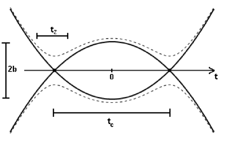
Figure 1: The two-level parabolic model. Solid lines are the diabatic energy levels as a function of time, and dashed lines are the adiabatic energy levels (featuring an avoided crossings). We choose the scaled coupling $b>0$ in order to have a double crossing case. The Zener time $t_{Z}$ and the crossing separation $t_{c}$ are also shown.

We now discuss the two-level parabolic model Bykhovskii65 ; Crothers77 ; Shimshoni91 ; Suominen92 and its extensions to a higher number of levels. The Hamiltonian of the parabolic model is

$$H_{Para}^{(2)}=\left(\begin{array}[]{cc}at^{2}-b&v\\ v&-at^{2}+b\\ \end{array}\right),$$ (14)

where $a$ and $v$ are positive and $b$ is a real number. The sign of $b$ determines whether we have a double crossing ($b>0$), a single crossing ($b=0$), or a tunneling case ($b<0$). In this paper we will consider only the $b>0$ case (Fig. 1). In terms of the spin-1/2 operators the parabolic Hamiltonian can be written as $H_{Para}^{(2)}=2v\,S_{x}^{(2)}+2(at^{2}-b)S_{z}^{(2)}$. It is convenient to scale the system by defining a dimensionless time $\tau=vt/\hbar$ which leads to the new Hamiltonian

$$\bar{H}_{Para}^{(2)}=\left(\begin{array}[]{cc}\epsilon\tau^{2}-\mu&1\\ 1&-\epsilon\tau^{2}+\mu\\ \end{array}\right),$$ (15)

where $\epsilon=\hbar^{2}a/v^{3}$ and $\mu=b/v$ are dimensionless parameters Suominen92 .

Analytic solutions for the propagator $U^{(2)}_{Para}(+\infty,-\infty)$ have been presented in the literature Shimshoni91 ; Suominen92 in some limiting cases. Reference Suominen92 provides an analytic solution in the adiabatic limit, using the interaction picture and the adiabatic basis representation. If generalized, this solution suggests that more generally, if condition (13) is satisfied, so that the two resonances can be treated as independent linear crossings (ICA), their contribution can be described by the Landau-Zener propagator of Eq. (7). Linearizing $\bar{H}_{Para}^{(2)}$ at the crossings we find that the associated Zener time is given in terms of the scaled time as

$$\tau_{Z}=\left\{\begin{array}[]{ll}\frac{1}{2\sqrt{\mu\epsilon}},&2\sqrt{\mu\epsilon}\ll 1,\\ \\ \sqrt{\frac{1}{2\sqrt{\mu\epsilon}}},&2\sqrt{\mu\epsilon}\gg 1,\end{array}\right.$$ (16)

with the upper line corresponding to the adiabatic and the lower line to the sudden limit. The distance between the crossings is $\tau_{c}=2\sqrt{\mu/\epsilon}$. Thus the ICA condition (13) is satisfied when $\mu\gg 1$ (adiabatic limit) or $(\mu^{3}/\epsilon)^{1/4}\gg 1$ (sudden limit).

We assume that between the crossings only the phase evolves. The propagator relative to this evolution reads

$$U_{ph}^{(2)}=\left(\begin{array}[]{cc}e^{-i\sigma/2}&0\\ 0&e^{i\sigma/2}\\ \end{array}\right),$$ (17)

where $\sigma$ characterizes the adiabatic dynamical phase. As it is found out in Suominen92 and confirmed by our numerical calculations, the propagator obtained in this way works very well when ICA is satisfied. The total propagator in the interaction picture can be written as

$$U_{Para}^{(2)}(+\infty,-\infty)=U_{LZ}^{T(2)}U_{ph}^{(2)}U_{LZ}^{(2)}=\left(\begin{array}[]{cc}\alpha&\beta\\ -\beta^{*}&\alpha^{*}\\ \end{array}\right),$$ (18)

where $U_{LZ}^{T(2)}$ indicates the transpose of (7). The reason of using the transpose lies in the fact that after the first crossing one of the adiabatic states changes sign. Thus the propagator at the second crossing needs to be written in the new adiabatic basis. We need to change the signs of the non-diagonal elements of (7), or equivalently in our case, to take its transpose.

In Eq. (18) we have

$$\alpha = e^{i\sigma/2}[R^{2}+e^{-i(\sigma+2\phi)}(1-R^{2})],$$ (19)

$$\beta = 2iR\sqrt{1-R^{2}}\sin(\phi+\sigma/2).$$ (20)

Here $R$ and $\phi$ are obtained from Eqs. (8) and (10) by defining

$$\Lambda=\frac{1}{2\sqrt{\epsilon\mu}},\qquad R=\exp\left[-\frac{\pi}{4\sqrt{\epsilon\mu}}\right].$$ (21)

Additionally, the dynamical phase is obtained as

$$\sigma = 4\int_{0}^{\sqrt{\mu/\epsilon}}d\tau\,\sqrt{(\epsilon\tau^{2}-\mu)^{2}+1}$$ (22)

$$= \frac{2\tau_{c}}{3}\left\{1+2\sqrt{\frac{\mu+i}{\mu}}\left(\mu\,\textrm{EE}\left[\arcsin\sqrt{\frac{\mu}{\mu-i}},\frac{\mu-i}{\mu+i}\right]\right.\right.$$

$$\left.\left.-i\textrm{EF}\left[\arcsin\sqrt{\frac{\mu}{\mu-i}},\frac{\mu-i}{\mu+i}\right]\right)\right\}.$$

This is the full phase difference accumulated by the adiabatic states between the two crossings. Here EE stands for EllipticE and EF for EllipticF. These are defined as $\textrm{EllipticE}[\alpha,m]=\int_{0}^{\alpha}d\theta\,\sqrt{1-m\sin^{2}\theta}$ and $\textrm{EllipticF}[\alpha,m]=\int_{0}^{\alpha}d\theta\,1/\sqrt{1-m\sin^{2}\theta}$. Equation (22) shows that the dynamical phase $\sigma$ can be written as a product of $\tau_{c}$ and a function which only depends on $\mu$. When $\mu$ is large we can approximate $\sigma\approx 8\mu^{3/2}/(3\sqrt{\epsilon})=4\tau_{c}\mu/3$, which correspond to the value of $\sigma$ obtained in the absence of coupling. Therefore, when the energy separation between the two levels at $t=0$ is large compared with the coupling, it is possible to calculate the dynamical phase in the diabatic basis. This approximation has been used in Ref. Shimshoni91 in the derivation of an approximate propagator for the parabolic model. However, when the exact result (22) is used, the resulting propagator works well also when $v$ is not small compared with the energy separation at $t=0$.

As we noted with the LZ model, working in the interaction picture is a necessity due to the otherwise infinite dynamical phases. If we start either the LZ model or the parabolic model in a superposition of states in the Schrödinger picture, problems will arise. Since we are modelling here the idea of an interferometer, where the first beamsplitter creates the superposition, we can avoid the infinite phase problem by restricting our study to situations where only a single eigenstate on the system is populated initially.

In a two-level model, starting from level $1$, the transition probability to level $2$ is now

$$P^{(2)}_{1\rightarrow 2}=|\beta|^{2}=4R^{2}(1-R^{2})\sin^{2}(\sigma/2+\phi).$$ (23)

We note that the expression for $P^{(2)}_{1\rightarrow 2}$ given in Ref. Suominen92 contains misprints, the correct form is given by Eq. (23).

As an example we discuss the generalization of the parabolic model to three-level systems. The Hamiltonian is now

$$H_{Para}^{(3)}=\left(\begin{array}[]{ccc}2(at^{2}-b)&\sqrt{2}v&0\\ \sqrt{2}v&0&\sqrt{2}v\\ 0&\sqrt{2}v&-2(at^{2}-b)\end{array}\right),$$ (24)

Using Eq. (II) together with Eq. (18) we find the solution for a three-level system propagator as

$$U^{(3)}_{Para}=\left(\begin{array}[]{ccc}\alpha^{2}&\sqrt{2}\alpha\beta&\beta^{2}\\ -\sqrt{2}\alpha\beta^{*}&|\alpha|^{2}-|\beta|^{2}&\sqrt{2}\alpha^{*}\beta\\ \beta^{*2}&-\sqrt{2}\alpha^{*}\beta^{*}&\alpha^{*2}\\ \end{array}\right),$$ (25)

where $\alpha$ and $\beta$ are given by Eqs. (19) and (20). Starting again with level $1$ initially populated we find that the transition probability to level $3$ is

$$P^{(3)}_{1\rightarrow 3}=|\beta|^{4}=16R^{4}(1-R^{2})^{2}\sin^{4}(\sigma/2+\phi).$$ (26)

If we ignore the rather small $\Lambda$-dependence of $\phi$, we see that the parameter $\Lambda$ controls the amplitude, and the oscillations arise only from $\sigma$.

IV Interferometry using spinor condensates

IV.1 Theoretical analysis

The order-parameter of a spin-$F$ condensate can be written as

$$\psi(t)=\sum_{m_{F}=-F}^{F}\psi_{m_{F}}(\mathbf{r},t)\displaystyle{|F,m\rangle},$$ (27)

with the normalization $\sum_{m_{F}=-F}^{F}|\psi_{m_{F}}(\mathbf{r},t)|^{2}=n(\mathbf{r},t)$, where $n(\mathbf{r},t)$ is the total particle density. We assume that the condensate is confined in an optical dipole trap so that all the components of the hyperfine spin can be trapped simultaneously, and they are degenerate in the absence of any magnetic fields. In the following we concentrate on an $F=1$ condensate. In the degenerate case the time-evolution of an $F=1$ condensate is given by the following set of time-dependent Gross-Pitaevskii equations Machida ; Ho ; Isoshima

$$i\hbar\frac{\partial\psi_{1}}{\partial t} = {\cal L}\psi_{1}+\lambda_{a}\left(\psi_{0}^{2}\psi_{-1}^{*}+|\psi_{1}|^{2}\psi_{1}+|\psi_{0}|^{2}\psi_{1}\right.$$

$$\left.-|\psi_{-1}|^{2}\psi_{1}\right),$$

$$i\hbar\frac{\partial\psi_{0}}{\partial t} = {\cal L}\psi_{0}+\lambda_{a}\left(2\psi_{1}\psi_{-1}\psi_{0}^{*}+|\psi_{-1}|^{2}\psi_{0}+|\psi_{1}|^{2}\psi_{0}\right),$$

$$i\hbar\frac{\partial\psi_{-1}}{\partial t} = {\cal L}\psi_{-1}+\lambda_{a}\left(\psi_{0}^{2}\psi_{1}^{*}+|\psi_{-1}|^{2}\psi_{-1}+|\psi_{0}|^{2}\psi_{-1}\right.$$ (28)

$$\left.-|\psi_{1}|^{2}\psi_{-1}\right),$$

with ${\cal L}=-\hbar^{2}\nabla^{2}/(2m)+U(\mathbf{r},t)+\lambda_{s}n(\mathbf{r},t)$, $\lambda_{s}=4\pi\hbar^{2}(a_{0}+2a_{2})/(3m)$ and $\lambda_{a}=4\pi\hbar^{2}(a_{2}-a_{0})/(3m)$. The $a_{k}$’s are the $s$-wave scattering lengths in the scattering channels with total spin $k$. The trapping potential is denoted by $U$, and it affects all spinor components equivalently. The first term inside each parentheses describes spin mixing processes where atoms in $m_{F}=+1$ and $m_{F}=-1$ states collide and create two atoms in $m_{F}=0$ state, or vice versa. The number of particles in the $i$th component is by definition $N_{i}\equiv\int d^{3}r\,|\psi_{i}|^{2}$. From Eqs. (28) we get

$$\frac{\partial N_{1}}{\partial t}=\frac{\partial N_{-1}}{\partial t}=-\frac{1}{2}\frac{\partial N_{0}}{\partial t}=\frac{2\lambda_{a}}{\hbar}\int d^{3}r\,\textrm{Im}[\psi_{0}^{2}\psi^{*}_{-1}\psi^{*}_{1}].$$ (29)

It follows that

$$\left|\frac{\partial N_{0}}{\partial t}\right|<\gamma N_{0},\quad\gamma\equiv\frac{4|\lambda_{a}|n_{max}}{\hbar},$$ (30)

where $n_{max}$ is the maximum density. Using the scattering lengths relevant for ⁸⁷Rb vanKempen02 and a maximum density $n_{max}=10^{14}\textrm{ cm}^{-3}$ we find $\gamma\simeq 90\ s^{-1}$. If for example we have $\Delta t=100\ \mu$s the change in the populations is less than 1 %. The time-evolution given by the Gross-Pitaevskii equations (28) is then restricted to changes in the phases of the spinor components. Thus we can describe it defining the following effective propagator

$$U_{GP}^{(3)}=\left(\begin{array}[]{ccc}e^{i\theta_{1}}&0&0\\ 0&1&0\\ 0&0&e^{-i\theta_{-1}}\\ \end{array}\right),$$ (31)

where we set one of the three independent phases to zero. The phases $\theta_{1}$ and $\theta_{-1}$ can be calculated by solving Eqs. (28).

IV.2 The spinor interferometer

We base our interferometer proposal for the analogy between optical beamsplitters and the level crossings. The initial single-state signal is split into two parts at the splitter-crossing. The two parts travel along the different arms of the interferometer, and combine again in the second splitter-crossing, to form a detectable signal. Thus any difference in phase evolution along the two paths is mapped into variation of populations. The closest counterpart of our spinor interferometer is the quantum optical Mach-Zehnder interferometer. In our case, however, the interferometer can have more than two arms.

Let us consider a few points in our analogue. The splitting at the level crossings can be controlled by the speed of change for the bias field and by the coupling field strength. Thus we are not limited to the 50-50 splitting. Here the controlling parameter is the Landau-Zener term $R$. As for the phase evolution, Eq. (26) demonstrates that it decouples from the splitting, although we must remember that the standard phase evolution $\sigma$ will depend on the same parameters as $R$. On the other hand, we have altogether three parameters [$a$, $b$ and $v$ in Eq. (14)], so it is possible to fix $R$ and $\sigma$ independently.

The time-evolution of spinor states between the crossings represents the internal part of the spinor interferometer. This is the time region during which the phenomena to be investigated take place. As discussed earlier, we consider temporal crossing separations which are much shorter than the typical time scales of spin mixing processes. Thus we suggest that the contribution (31) is included to the total propagator, which becomes now

$$U_{TOT}^{(3)}=U_{LZ}^{T(3)}U_{ph}^{(3)}U_{GP}^{(3)}U_{LZ}^{(3)},$$ (32)

where $U_{ph}^{(3)}$ is obtained from (17) through Eq. (II). Thus the solution is obtained as a sequence of separate events.

It is important to notice that the propagator (18) is written in the adiabatic basis while (31) is written in the diabatic basis [following Eqs. (28)]. But the result (32) is still well-defined. The reason lies in the ICA approximation. Since $v\ll b$, the adiabatic and diabatic state evolution coincide approximately outside the crossing regions. The only problem arises in the vicinity of the crossings, but these time intervals are much shorter ($t_{Z}\ll t_{c}$) and do not contribute much to the phase evolution.

As an example let us start with the state $\displaystyle{|1,1\rangle}$ initially populated. The final population of the state $\displaystyle{|1,-1\rangle}$ is

$$P^{(3)}_{1\rightarrow-1}=16R^{4}(1-R^{2})^{2}\left\{\sin^{4}\chi+\cos 2\chi\sin^{2}\Psi\right\},$$ (33)

where

$$\chi\equiv\frac{\sigma}{2}+\phi-\frac{\theta_{1}+\theta_{-1}}{4},\qquad\Psi\equiv\frac{\theta_{1}-\theta_{-1}}{4}.$$ (34)

The result (33) depends on the parameters $\sigma$ and $\phi$, which one can control externally, and on the GP phases $\theta_{1}$ and $\theta_{-1}$. Thus the measure of the final population of the $\displaystyle{|1,-1\rangle}$ state (the output of the interferometer) gives information on the Gross-Pitajevskii dynamics. We can also see that the visibility of the interferometric oscillations is maximized when $R=1/\sqrt{2}$.

A simple interferometric measurement would be thus to set $R=1/\sqrt{2}$ to maximize the signal, then to vary $\chi$ (keeping $R$ constant). As one can see from Eq. (33), the difference between minima and maxima gives information about $\Psi$. Interestingly, possible fluctuations in the magnetic fields affect the Zeeman shifts between adjacent spinor states equally, thus affecting only $\sigma$.

One should note that because of the $\sin^{4}$-function, the fringes are ”sharper” than in the standard two-arm interferometer. If we go to higher values of spin, such as $F=2$, the fringes become even sharper. In analogy to diffraction patterns, the double slit is replaced by a $2F+1$-slit. Note that in this case the number of independent relative phases is $2F$.

IV.3 Experimental realization

In this section we estimate the values of the parameter of the interferometer looking at a real situation. The effect of the interaction with an external magnetic field is described by the general linear Zeeman model

$$H_{B}^{(3)}=-g_{F}\mu_{B}\mathbf{B}\cdot\mathbf{\hat{F}},$$ (35)

where $\mu_{B}$ is the Bohr magneton, $g_{F}$ is the Lande $g$-factor (equal to 1/2 for ⁸⁷Rb and ²³Na), $\mathbf{B}=(B_{x},B_{y},B_{z})$ is the magnetic field, and $\mathbf{\hat{F}}=(F_{x},F_{y},F_{z})$ is the spin operator of a spin-1 particle (with $\hbar=1$). We can identify $H_{B}^{(3)}$ with $H_{Para}^{(3)}$ defining $B_{x}=-4v/\mu_{B}$, $B_{y}=0$, and $B_{z}=-4(at^{2}-b)/\mu_{B}$. With these definitions we get ($g_{F}=1/2$)

$$\mu = \frac{|B_{z}(t=0)|}{B_{x}},$$

$$\epsilon\mu = \left(\frac{2\hbar\dot{B}_{z}^{c}}{\mu_{B}B_{x}^{2}}\right)^{2},$$ (36)

$$t_{c} = \frac{4|B_{z}(t=0)|}{|\dot{B}_{z}^{c}|},$$

where $|\dot{B}_{z}^{c}|$ is the rate of change of $B_{z}(t)$ at the crossings. The Zener time becomes

$$t_{Z}=\left\{\begin{array}[]{ll}\frac{B_{x}}{2\dot{B}_{c}},&\frac{4\hbar\dot{B}_{z}^{c}}{\mu_{B}B_{x}^{2}}\ll 1,\\ &\\ \sqrt{\frac{2\hbar}{\mu_{B}\dot{B}_{z}}},&\frac{4\hbar\dot{B}_{z}^{c}}{\mu_{B}B_{x}^{2}}\gg 1.\end{array}\right.$$ (37)

We estimate the values of $\epsilon$ and $\mu$ by choosing $B_{x}=60$ mG and $\dot{B}_{z}^{c}=5\cdot 10^{4}$ G/s, and $B_{z}(0)=300$ mG. These give $\epsilon\approx 2$ and $\mu=5$. The distance between the crossings is $t_{c}=24\ \mu$s while the Zener time is $t_{LZ}\approx 2\ \mu$s, which shows that the ICA is well satisfied, and our approach should be applicable. From the previous values we also get $R\approx 0.78$ which is very close to the value $1/\sqrt{2}$ which maximizes the interferometric signal in (33).

In our experimental scenario we have considered a constant coupling field. Alternatively, we could use an rf-field scenario in analogy to evaporative cooling Pethick2008 . By performing the rotating wave approximation and moving to a rotaing coordinate frame we get a situation that is euivalent to the constant coupling field scenario. Then the crossings take place when the bias-field-induced Zeeman shifts become resonant with the rf-frequency, and the bias field does not have to pass a zero-point value. Yet another variation would involve chirping of the rf-frequency, as it can also be described as time-dependent variation of the energy of the spinor states.

V Conclusions

In this paper we have presented the basic idea of a spinor interferometer. It is based on applying time-dependent magnetic fields to provide level crossings of spinor states in analogy to optical beam splitters. Interferometer-like studies that apply the Landau-Zener model twice and show path-related interference are not uncommon in physics, see e.g. Ref. Sillanpaa06 . The spinor interferometer is a partial extension into the case of a multi-arm interferometer, which is perhaps harder to realize in quantum optics. The extension is only partial due to the nature of the spinor. For spin-$F$ we get $2F+1$ paths and $2F$ independent phases, but the spinor dynamics is nevertheless characterized by the same small number of parameters as the corresponding two-state model, as the Majorana representation shows. Instead of being a limitation, one can see this spinor property as an advantage when considering possible error sources.

It should also be clear that one is not limited to the parabolic model. We have chosen to use it because then we can link the intuitive concept of using the LZ model twice within ICA to the full solution of the model in the adiabatic limit, as done in Ref. Suominen92 . Our next step is to consider more carefully how the dynamics of Eqs. (28) appear in the phase evolution given by Eq. (31).

- (1) D. M. Stamper-Kurn, M. R. Andrews, A. P. Chikkatur, S. Inouye, H.-J. Miesner, J. Stenger, and W. Ketterle, Phys. Rev. Lett. 80, 2027 (1998).
- (2) T. Ohmi and K. Machida, J. Phys. Soc. Jap. 67, 1822 (1998).
- (3) T.-L. Ho, Phys. Rev. Lett. 81, 742 (1998).
- (4) C. K. Law, H. Pu, and N. P. Bigelow, Phys. Rev. Lett. 81, 5257 (1998).
- (5) H. Pu, C. K. Law, S. Raghavan, J. H. Eberly, and N. P. Bigelow, Phys. Rev. A 60, 1463 (1999).
- (6) E. Majorana, Nuovo Cimento 9, 43 (1932).
- (7) L. D. Landau, Phys. Z. Sowjet Union 2, 46 (1932).
- (8) C. Zener, Proc. R. Soc. Lond. A 137, 696 (1932).
- (9) K.-A. Suominen, Opt. Comm. 93, 126 (1992).
- (10) F. Bloch and I. I. Rabi, Rev. Mod. Phys. 17, 237 (1945).
- (11) N. V. Vitanov and K.-A. Suominen, Phys. Rev. A 56, R4377 (1997).
- (12) L. Xia, X. Xu, R. Guo, F. Yang, W. Xiong, J. Li, Q. Ma, X. Zhou, H. Guo, and X. Chen, Phys. Rev. A 77, 043622 (2008).
- (13) C. Gerry and P. Knight, Introductory Quantum Optics (Cambridge University Press, Cambridge, 2005).
- (14) A. Meckler, Phys. Rev. 111, 1447 (1958).
- (15) A. P. Kazantsev, G. I. Surdutovich, and V. P. Yakovlev, Mechanical Action of Light on Atoms (World Scientific, Singapore, 1990).
- (16) K. Mullen, E. Ben-Jacob, Y. Gefen, and Z. Schuss, Phys. Rev. Lett. 62, 2543 (1989).
- (17) V. K. Bykhovskii, F. F. Nikitin, and M. Ya. Ovchinnikova, Sov. Phys. JETP 20, 500 (1965).
- (18) D. S. F. Crothers and J. G. Hughes, J. Phys. B: Atom. Molec. Phys. 10, L557 (1977).
- (19) E. Shimshoni and Y. Gefen, Ann. Phys. (N.Y) 210, 16 (1991).
- (20) T. Isoshima, M. Nakahara, T. Ohmi, and K. Machida, Phys. Rev. A 61, 063610 (2000).
- (21) E. G. M. van Kempen, S. J. J. M. F. Kokkelmans, D. J. Heinzen, and B. J. Verhaar, Phys. Rev. Lett. 88, 093201 (2002).
- (22) C. J. Pethick and H. Smith, Bose-Einstein Condensation in Dilute Gases, 2nd ed. (Cambridge University Press, Cambridge, 2008).
- (23) M. Sillanpää, T. Lehtinen, A. Paila, Y. Makhlin, and P. Hakonen, Phys. Rev. Lett. 96, 187002 (2006).