Partons and jets in a strongly–coupled plasma from AdS/CFT

Abstract:

We give a pedagogical review of recent progress towards understanding the response of a strongly coupled plasma at finite temperature to a hard probe. The plasma is that of the ${\mathcal{N}}=4$ supersymmetric Yang–Mills theory and the hard probe is a virtual photon, or, more precisely, an ${\mathcal{R}}$–current. Via the gauge/gravity duality, the problem of the current interacting with the plasma is mapped onto the gravitational interaction between a Maxwell field and a black hole embedded in the $AdS_{5}\times S^{5}$ geometry. The physical interpretation of the AdS/CFT results can be then reconstructed with the help of the ultraviolet/infrared correspondence. We thus deduce that, for sufficiently high energy, the photon (or any other hard probe: a quark, a gluon, or a meson) disappears into the plasma via a universal mechanism, which is quasi–democratic parton branching: the current develops a parton cascade such that, at any step in the branching process, the energy is almost equally divided among the daughter partons. The branching rate is controlled by the plasma which acts on the colored partons with a constant force $\sim T^{2}$. When reinterpreted in the plasma infinite momentum frame, the same AdS/CFT results suggest a parton picture for the plasma structure functions, in which all the partons have fallen at very small values of Bjorken’s $x$. For a time–like current in the vacuum, quasi–democratic branching implies that there should be no jets in electron–positron annihilation at strong coupling, but only a spatially isotropic distribution of hadronic matter.

1 Introduction: From RHIC physics and lattice QCD to AdS/CFT

One of the most interesting suggestions emerging from the heavy ion program at RHIC is the fact that the deconfined, ‘quark–gluon’ matter produced in the early stages of an ultrarelativistic nucleus–nucleus collision might be strongly interacting (see the summary of the experimental results in the “white papers” of the four experiments at RHIC [1, 2, 3, 4] and the review articles [5, 6, 7, 8, 9] for discussions of their theoretical interpretations). This represents an important paradigm shift, since the prevalent opinion for quite some time was that this form of hadronic matter should be weakly coupled, because of its high density and of the asymptotic freedom of QCD. This shift of paradigm intervened only a few years after the recognition of the AdS/CFT correspondence [10, 11, 12, 13] — a theoretical revolution which offered a whole new framework, based on string theory, to address problems in strongly coupled gauge theories. The advent of the RHIC data has motivated an intense theoretical activity over the last few years, aiming at using the AdS/CFT correspondence to understand properties of QCD–like matter at finite temperature and/or high energy (see, e.g., the recent review paper [14] and Refs. therein).

One should emphasize here that the experimental evidence in favour of strong–coupling dynamics at RHIC is rather indirect — its physical interpretation also involves theoretical assumptions which are generally model–dependent —, but some of the data seem quite robust and compelling. This is especially the case for those which reflect the long–range, collective properties of the hadronic matter. For instance, the RHIC data exhibit a form of collective motion called ‘elliptic flow’ [15], which demonstrates that the partonic matter produced in the early stages of a Au+Au collision behaves like a fluid. Remarkably, these data can be well accommodated within theoretical analyses using hydrodynamics, which assume early thermalization and nearly zero viscosity — or, more precisely, a very small viscosity to entropy–density ratio $\eta/s$. These features are hallmarks of a system with very strong interactions: indeed, at weak coupling $g\ll 1$, the equilibration time and the ratio $\eta/s$ are both parametrically large, since proportional to the mean free path $\sim 1/g^{4}$. On the other hand, AdS/CFT calculations for gauge theories with a gravity dual [16] suggest that, in the limit of an infinitely strong coupling, the ratio $\eta/s$ should approach a universal lower bound which is $\hbar/4\pi$ [17]. (The existence of such a bound is also required by the uncertainty principle.) Interestingly, it appears that, within the error bars, the ratio $\eta/s$ extracted from the RHIC data [18, 19] is roughly consistent with this lower bound, thus supporting the new paradigm of a strongly coupled Quark–Gluon Plasma (sQGP).

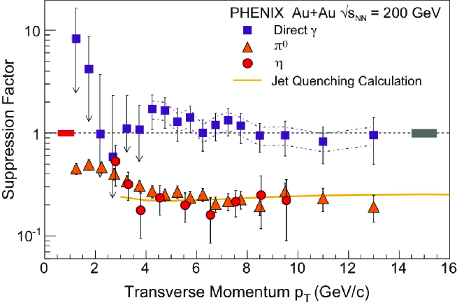
Figure 1: The ratio $R_{AA}$ of measured versus expected yield of various particles ($\pi^{0},\eta,\gamma$) in Au+Au collisions at $\sqrt{s_{\rm NN}}=200$ GeV as function of the transverse momentum $p_{T}$ (RHIC, PHENIX collaboration). Unlike the direct photons, the mesons shows a strong amount of suppression at high $p_{T}$, which is moreover the same for pions and $\eta$–mesons. This suggests that the suppression is an effect related to the absorption (energy loss) of energetic partons in the medium.

But experimental indications in favour of strong interactions have also emerged from different type of data — those associated with hard probes. A ‘hard process’ in QCD is a scattering involving a large momentum exchange, $Q\gg\Lambda_{{\rm QCD}}\sim 200$ MeV. In the context of heavy ion collisions, the ‘hard probes’ are highly energetic ‘jets’ (partons, virtual photons, dileptons, heavy–quark mesons), which are produced by the hard scattering of the incoming quarks and gluons, and which on their way towards the detectors measure the properties of the surrounding matter with a high resolution, meaning on very short space–time scales. One would expect such hard interactions to lie within the realm of perturbative QCD, yet some of the experimental results at RHIC seem difficult to explain by perturbative calculations at weak coupling. One of these results is the ratio $R_{AA}$ between the particle yield in Au+Au collisions and the respective yield in proton–proton collisions rescaled by the number of participating nucleons. This ratio would be one if a nucleus–nucleus collision was the incoherent superposition of collisions between the constituents nucleons (protons and neutrons) of the two incoming nuclei. But the RHIC measurements show that $R_{AA}$ is close to one only for direct photon production, whereas for hadron production it is strongly suppressed (roughly, by a factor of 5; see Fig. 1). This suggests that, after being produced through a hard scattering, the partonic jets are somehow absorbed by the surrounding medium.

  

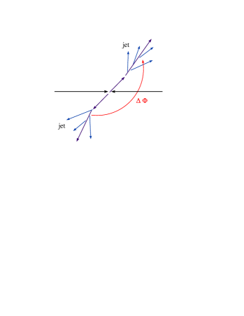
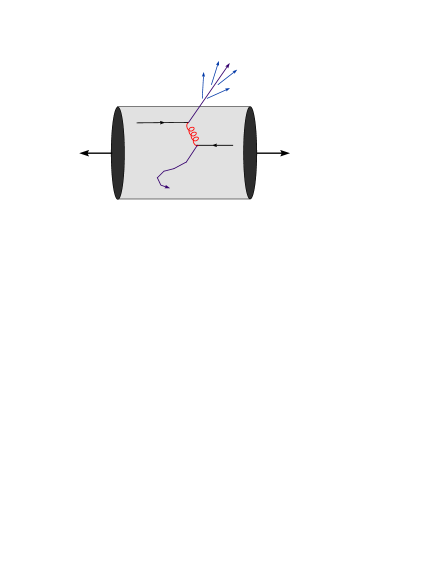
Figure 2: Jet production in high–energy scattering. Left: the typical situation in a proton–proton collision: the leading partons fragment into two back–to–back hadronic jets, which are both observed by the detector. Right: a nucleus–nucleus collision: one of the leading partons escapes the interaction region and yields a jet in the detector, but the other one is absorbed by the surrounding matter.

Additional evidence in that sense comes from studies of jets and, more precisely, of the angular correlation of the radiation associated with a trigger particle with high transverse momentum (the ‘near side jet’). A high–energy proton–proton (or electron–positron) collision generally produces a pair of partons whose subsequent evolution (through fragmentation and hadronisation) leaves two jets of hadrons which propagate back–to–back in the center of mass frame (see Fig. 2 left). Hence, if one uses a hard particle in one of these jets to trigger the detector, then the distribution of radiation in the azimuthal angle $\Delta\Phi$ shows two well pronounced peaks, at $\Delta\Phi=0$ and $\Delta\Phi=\pi$, as shown in Fig. 3 (the curve denoted there as ‘p+p min. bias’). A similar distribution is seen in deuteron–gold collisions (the points d+Au in Fig. 3), but not in central Au+Au collisions, where the peak at $\Delta\Phi=\pi$ (the ‘away side jet’) has disappeared, as shown by the respective RHIC data in Fig. 3. It is then natural to imagine that the hard scattering producing the jets has occurred near the edge of the interaction region, so that the near side jet has escaped to the detector, while the away side jet has been absorbed while crossing through the medium (see Fig. 2 right).

The Au+Au results in Figs. 1 and 3 show that the matter produced right after a heavy ion collision is opaque, which may well mean that this matter is dense, or strongly–coupled, or both. The theoretical way to describe the disappearance of a parton in this matter is by computing the rate for energy loss ${\rm d}E/{\rm d}t$, which is proportional to a specific transport coefficient — the ‘jet quenching parameter’ $\hat{q}$ — which characterizes the parton interactions in the medium (see, e.g., [8] and Refs. therein). This extraction of this parameter from the RHIC data is accompanied by large uncertainties, so the obtained values lies within a wide window: $\hat{q}\,\simeq\,0.5\div 15$ ${\rm GeV}^{2}/{\rm fm}$ (see, e.g., [20, 21]). It is often stated that this value is too large to be accommodated by weak coupling calculations, but this is still under debate [22]. What is clear, however, is that a complimentary analysis of these phenomena in the non–perturbative regime at strong coupling would be highly valuable, and this is where the AdS/CFT correspondence comes into the play.

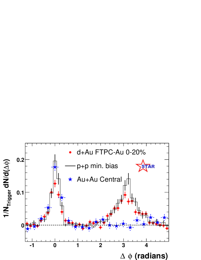
Figure 3: Azimuthal correlations for jet measurements at RHIC (STAR collaboration) in p+p, d+Au, and Au+Au collisions. The selected events are such that the trigger particle has transverse momentum 4 GeV $<p_{T}<$ 6 GeV and the associated radiation has $p_{T}>$ 2 GeV.

The standard non–perturbative technique in QCD, which is lattice gauge theory, is not applicable (at least, in its current formulation) for dynamical observables, so like real–time evolution, transport coefficients, or interaction rates. On the other hand, such problems can be addressed via the AdS/CFT correspondence, but the applicability of the latter is restricted to the limit where the ‘t Hooft coupling is strong $\lambda\equiv g^{2}N_{c}\gg 1$ (which in practice means a large number of colors: $N_{c}\gg 1$), and to special gauge theories which are more symmetric than QCD and for which a ‘gravity dual’ (i.e., an alternative representation as a string theory living in a curved space–time geometry in $D=1+9$ dimensions) has been identified. The original, and so far best established, such duality is that between the ${\mathcal{N}}=4$ supersymmetric Yang–Mills (SYM) theory and the type IIB superstring theory living in a background geometry which is asymptotically $AdS_{5}\times S^{5}$ [10, 11, 12] (see Sect. 3 below). The ${\mathcal{N}}=4$ theory is a priori quite different from her QCD ‘cousin’ : it is maximally supersymmetric, it has conformal symmetry at quantum level (meaning that the coupling is fixed), it has no confinement (and hence no hadronic asymptotic states), and the fields in the Lagrangian are all in the adjoint representation of the ‘colour’ gauge group SU$(N_{c})$ (unlike QCD, where the fermions lie in the fundamental representation). So the relevance of the AdS/CFT results for our real world is generally far from being clear. Yet, the particular context of ultrarelativistic heavy ion collisions, as explored at RHIC and in the near future at LHC, is quite exceptional in that respect, because many of the limitations of the AdS/CFT correspondence become less important in this context.

  

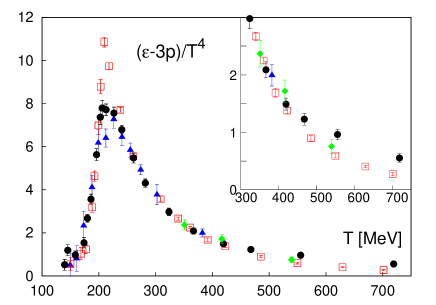
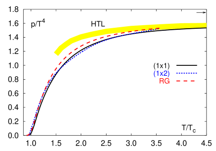
Figure 4: Lattice results for the trace anomaly, $T^{\mu}_{\mu}=\epsilon-3p$, in units of $T^{4}$ (left) [23] and for the pressure of the SU$(3)$ gauge theory (right) [24]. In the right figure, different lines correspond to different gauge actions, whereas the upper band denoted as ‘HTL’ (for ‘Hard Thermal Loop’) represents the results of a parameter–free resummation of perturbation theory [25]. The small arrow in the upper right corner indicated the pressure of an ideal gas, i.e., the zero–coupling limit $g\to 0$.

Indeed, the QCD matter of interest is anyway in a deconfined, quark–gluon plasma, phase, for which the ‘conformal anomaly’ — the breaking of the conformal symmetry of the QCD Lagrangian by the running of the coupling — appears to be relatively small. This is confirmed by lattice simulations for the QCD thermodynamics within the temperature range corresponding to the energy density produced at RHIC and (in perspective) LHC: the relevant range for $T$ is $2T_{c}\leq T\leq 5T_{c}$, where $T_{c}\simeq\Lambda_{{\rm QCD}}\simeq 200$ MeV is the critical temperature for the deconfinement phase transition. The running of the QCD coupling $g(\mu)$ is negligible within such a restricted range and, besides, the relevant value turns out to be quite large: $g\gtrsim 1.5$, meaning $\lambda\gtrsim 6$, which leaves the hope for a strong–coupling behaviour. Moreover, the lattice calculation of the ‘trace anomaly’ $\langle T^{\,\mu}_{\mu}\rangle$, which is proportional to the QCD $\beta$–function,

$$\langle T^{\,\mu}_{\mu}\rangle\,=\,\epsilon-3p\,=\,\beta(g)\,\frac{{\rm d}p}{{\rm d}g}\,,$$ (1.1)

($\epsilon$ is the energy density and $p$ is the pressure) yields a relatively small result — less than 10% of the total energy density — for all temperatures above $2T_{c}\simeq 400$ MeV (see Fig. 4 left).

But lattice QCD at finite temperature also illustrates the difficulty to decide whether the quark–gluon plasma is strongly–coupled, or not, within the relevant range of temperatures. To explain this, consider the lattice results for the pressure, as shown in Fig. 4 (right): after a sharp increases around $T_{c}$, the QCD pressure is slowly approaching, for temperatures $T\gtrsim 1.5T_{c}$, towards the corresponding value $p_{0}$ for an ideal gas, which in Fig. 4 (right) is indicated by the small arrow in the upper right corner. As visible in this figure, the deviation $(p-p_{0})/p_{0}$ is quite small, less than $20\%$, for all temperatures $T\gtrsim 2T_{c}$. One may thus conclude that the QGP is weakly coupled at these temperatures. And, indeed, a weak–coupling calculation [25], based on a resummation of the perturbation theory and whose results are indicated by the upper, ‘HTL’, band in Fig. 4 right, provides a rather good description of the lattice results for $T\gtrsim 2.5T_{c}$. However, this conclusion is challenged by the AdS/CFT calculation of the pressure in the ${\mathcal{N}}=4$ SYM plasma in the strong coupling limit $\lambda\to\infty$ [26], which yields a remarkable result : the pressure at infinite coupling is exactly 3/4 of the corresponding ideal–gas value $p_{0}$ :

$$p(\lambda\to\infty)\,=\,\frac{\pi^{2}}{8}\,N_{c}^{2}T^{4}\,=\,\frac{3}{4}\,p_{0}\,.$$ (1.2)

This ratio $p/p_{0}=0.75$ is close to the value $p/p_{0}\approx 0.85$ found in lattice QCD at $T=2.5T_{c}$ (see Fig. 4 right), so the latter might be consistent with strong coupling as well !

Since the lattice QCD results cannot be unambiguously interpreted, it is interesting to have a closer look at the ${\mathcal{N}}=4$ SYM theory at large $N_{c}$, for which both weak–coupling and strong–coupling calculations are possible. The corresponding expansions are known to next–to–leading order, i.e., to $\mathcal{O}{(\lambda^{3/2})}$ at weak coupling [27] and, respectively, $\mathcal{O}{(\lambda^{-3/2})}$ at strong coupling [26], and can be summarized as follows (for the entropy density $s$, for convenience): writing $s=f(\lambda)s_{0}$ with $s_{0}=({2\pi^{2}}/{3})N_{c}^{2}T^{3}$ (the ideal gas value), one finds

$$f(\lambda) \,=\, 1-\,\frac{3}{2\pi^{2}}\lambda\,+\,\frac{\sqrt{2}+3}{\pi^{3}}\lambda^{3/2}\,+\ldots\quad\mbox{for small $\lambda$\,,}$$ (1.3)

$$f(\lambda) \,=\, \frac{3}{4}\left(1+\frac{15\zeta(3)}{8}\lambda^{-3/2}+\ldots\right)\quad\mbox{for large $\lambda$}\,.$$ (1.4)

These expansions are illustrated in Fig. 5 [28], together with an interpolation between them which is nicely monotonic and can be viewed as the ‘true’ non–perturbative result (by lack of better approximations for intermediate values of the coupling). Also shown in Fig. 5 (the band denoted as ‘2PI’ there) is the result of a resummation of perturbation theory obtained via the same method as the ‘HTL’ band in Fig. 4 right. The resummation is necessary since, as also manifest in Fig. 5, the usual expansion in powers of $g$ (or $\lambda$) is poorly convergent and has no predictive power except at extremely small values of the coupling. This problem is generic to field theories at finite temperature, and is associated with collective phenomena which provide screening effects and thermal masses proportional to powers of $g$ ; the ‘resummations’ consist in keeping such medium effects within dressed propagators and vertices, instead of expanding them out in perturbation theory. (See the review papers [29] for more details and references.) As also visible in Fig. 5, the resummed perturbation theory yields a monotonic curve which matches with the ‘true’ result up to $\lambda\simeq 4$, where $s/s_{0}\simeq 0.85$. By comparison, the strong coupling expansion in Eq. (1.4) approaches the ‘true’ result only for $\lambda\gtrsim 8$. This suggests that a value $p/p_{0}\approx 0.85$ as found by lattice QCD around $2.5T_{c}$ truly corresponds to an intermediate value of the coupling (neither weak, nor strong), which is at least marginally within the reach of (properly organized) perturbation theory.

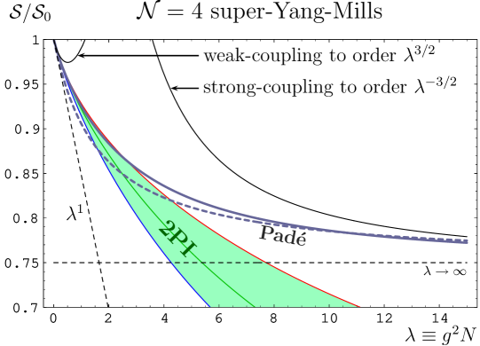
Figure 5: Weak and strong coupling results for the entropy density of $\mathcal{N}=4$ SYM theory together with the result of the resummed perturbation theory (the band denoted as ‘2PI’). The dashed and full heavy gray lines represent the Padé approximants $R_{[1,1]}$ and $R_{[4,4]}$ which interpolate between weak and strong coupling results to leading and next-to-leading orders, respectively.

To summarize, the lattice results for QCD thermodynamics at $T\gtrsim 2T_{c}$ do not provide strong evidence in favour of a strong–coupling dynamics, but they do not exclude it either. Moreover, the $\mathcal{N}=4$ SYM theory together with the AdS/CFT correspondance offers an unique opportunity to perform explicit calculations at both weak and strong coupling, with conclusions which may guide our interpretation of the corresponding results from lattice QCD. The purpose of these lectures is to present a similar guidance, but for a different physical problem: that of a ‘hard probe’ (a high–energy parton) propagating through a strongly–coupled $\mathcal{N}=4$ SYM plasma at finite temperature. There are clearly many differences between this idealized problem and the corresponding one in the phenomenology of heavy–ion collisions (like the replacement of QCD by the $\mathcal{N}=4$ SYM theory, or the assumption that the deconfined matter is at thermal equilibrium), but the crucial assumption in our opinion is that the coupling is strong. Thus, by comparing the conclusions of this AdS/CFT analysis with the respective data at RHIC (and in perspective LHC), and may hope to answer the following, fundamental question: is this particular regime of QCD mostly on the strong–coupling side, or on the weak–coupling one ?

In the recent literature, the problem of a hard probe propagating through a strongly coupled plasma has been addressed from different perspectives and within different approaches, depending upon the nature of the hard probe and of its string theory ‘dual’. The results of these various approaches appear to be consistent with each other at a fundamental level, and they point towards a universal mechanism for parton energy loss at strong coupling. Our main purpose in what follows will be to explain how this mechanism emerges from the results of the AdS/CFT calculations. To that aim we shall focus on the case where the ‘hard probe’ is a virtual photon (more precisely, an $\mathcal{R}$–current; see below) [30, 31]. This choice is motivated by simplicity: from the experience with QCD one knows that an electromagnetic current is the simplest device to produce and study hadronic jets. In deep inelastic scattering (DIS), the exchange of a highly virtual space–like photon between a lepton and a hadron acts as a probe of the hadron parton structure on the resolution scales set by the process kinematics. Also, the partonic fluctuation of a space–like current can mimic a quark–antiquark ‘meson’, which is nearly on–shell in a frame in which the current has a high energy. Furthermore, the decay of the time–like photon produced in electron–positron annihilation is the simplest device to produce and study hadronic jets in QCD. Thus, the propagation of an energetic current through the plasma gives access to quantities like the plasma parton distributions, the meson screening length, or the jet energy loss. The relation between our results for the virtual photon and the corresponding ones for other ‘hard probes’ — a heavy quark [32, 33, 34, 35, 36, 37, 38, 39], a quark–antiquark meson (built with heavy quarks) [40, 41, 42, 43, 44, 45, 46, 47], or a massless gluon [48, 49, 50] — will be described at appropriate places.

Within the ${\mathcal{N}}=4$ SYM theory, the role of the electromagnetic current is played by the ‘${\mathcal{R}}$–current’ — a conserved Abelian current whose charge is carried by fermion and scalar fields in the adjoint representation of the color group (see Sect. 3 for more details). Thus, DIS at strong coupling can be formulated as the scattering between this ${\mathcal{R}}$–current and some appropriate ‘hadronic’ target. The first such studies [51, 52] have addressed the zero–temperature problem, where the target was a ‘dilaton’ — a massless string state ‘dual’ to a gauge–theory ‘hadron’, whose existence requires the introduction of an infrared cutoff $\Lambda$ to break down conformal symmetry. These studies led to an interesting picture for the partonic structure at strong coupling: through successive branchings, all partons end up ‘falling’ below the ‘saturation line’, i.e., they occupy — with occupation numbers of order one — the phase–space at transverse momenta below the saturation scale $Q_{s}(x)$. This scale rises with $1/x$ as $Q_{s}^{2}(x)\sim 1/x$ which is much faster than for the corresponding scale in perturbative QCD [53]. This comes about because the high–energy scattering at strong coupling is governed by a spin $j\simeq 2$ singularity (corresponding to graviton exchange in the dual string theory), rather than the usual $j\simeq 1$ singularity associated with gluon exchange at weak coupling.

In Refs. [30, 31] these studies and the corresponding partonic picture have been extended to a finite–temperature ${\mathcal{N}}=4$ SYM plasma and also to the case of a time–like current (the strong–coupling analog of $e^{+}e^{-}$ annihilation). Note that this finite–$T$ case is conceptually clearer than the zero–temperature one, in that it does not require any ‘deformation’ of the gauge theory, like an IR cutoff. It is also technically simpler, in that the calculations can be performed in the strong ’t Hooft coupling limit $\lambda\equiv g^{2}N_{c}\to\infty$ at fixed $g^{2}\ll 1$ (meaning $N_{c}\to\infty$). This is so since the large number of degrees of freedom in the plasma, of order $N_{c}^{2}$ per unit volume, compensates for the $1/N_{c}^{2}$ suppression of the individual scattering amplitudes; hence, a strong–scattering situation can be achieved even in the strict large–$N_{c}$ limit. The AdS/CFT calculation shows that the saturation momentum of the plasma rises with the energy even faster than for a hadronic target, namely like $Q_{s}^{2}(x)\sim 1/x^{2}$. This difference is easily understood: the additional factor of $1/x$ is associated with the longitudinal extent of the interaction region, which for an infinite target (so like the plasma) grows with the energy, by Lorentz time dilation.

The results of Refs. [30, 31] will be described in Sects. 4 and 5 below, together with their physical interpretations. But before that, in Sect. 2, we shall briefly remind the perturbative QCD viewpoint on the simplest processes mediated by a virtual photon — $e^{+}e^{-}$ annihilation and DIS —, which will serve as a level of comparison for the corresponding discussion at strong coupling. Then, in Sect. 3, we shall give a succinct introduction to the AdS/CFT correspondence, whose purpose is not to be exhaustive — more details can be found in the review papers and textbooks listed in the references [13, 14, 54, 55] — but merely to present in a minimal but self–contained way that part of the formalism which is needed for our present purposes.

But more than describing the formalism, our main objective in these lectures is to present a physical picture for the dynamics at strong coupling, as originally proposed in Refs. [30, 31]. Building such a picture is generally difficult and in any case ambiguous, because of the lack of a direct connection between the AdS/CFT approach and the standard tools of quantum field theory, like Feynman diagrams. For the problem at hand, we shall rely on the intuition coming from perturbative QCD in order to propose a physical interpretation for the AdS/CFT results. But the most important tool in that sense will be the ultraviolet–infrared correspondence [56, 51, 57, 31], which relates the radial distance in $AdS_{5}$ to the virtuality of the partonic fluctuation created by the ${\mathcal{R}}$–current in the gauge theory. We feel that a more systematic use of this duality could provide more physical insight into other related calculations in the literature. For the same purpose, it turns out to be very useful to have a space–time representation for the dual processes in AdS/CFT, in addition to the more standard momentum–space picture, which is used to compute correlations. As we shall explain, via the UV/IR correspondence the space–time picture on the string theory side can be mapped onto an intuitive physical picture for the strong–coupling dynamics on the gauge theory side.

Our main physical conclusion is that a partonic interpretation for the high–energy processes makes sense even at strong coupling, and that the main mechanism for parton evolution in this regime is quasi–democratic parton branching, i.e., a successive branching process through which the energy of the incoming current, or parton, is rapidly and quasi–democratically divided among the daughter partons. This process takes place both in the vacuum (where, for instance, it leads to an isotropic distribution of particles in the final state of $e^{+}e^{-}$ annihilation, instead of the jet structure familiar in QCD), and in the finite–temperature plasma, where the rate for branching is influenced by the medium properties (we shall then speak of medium–induced parton branching). This branching process which, in the case of a plasma, continues until the partons have energies and virtualities of order $T$, represents the dominant mechanism for energy loss in the large–$N_{c}$ limit, where other mechanisms, like thermal rescattering, are suppressed.

2 Partons and jets in QCD at weak coupling

Before we turn to our main goal, which is a study of hard probes propagating through a strongly–coupled plasma, let us briefly discuss the situation in QCD, where hard scattering is rather associated with weak coupling. (More details on these pQCD topics can be found in textbooks like [58, 59].) By “hard scattering” we mean that the momentum transfer $Q$ in the collision (the scale which determines the relevant value of the QCD running coupling) is much larger than $\Lambda_{{\rm QCD}}\sim 200$ MeV, so that $\alpha_{s}(Q^{2})$ is reasonably small. (In practice, $Q^{2}\sim 4$ GeV² is already a ‘hard scale’, in which case $\alpha_{s}\simeq 0.25$.) We shall focus on processes which are mediated by a hard, virtual, electromagnetic current, since these are the processes that we shall later be interested in at strong coupling. At weak coupling at least, these are the processes in which the partonic picture of QCD is most directly revealed. In our subsequent discussion, we shall briefly review this picture and in particular emphasize those aspects which transcend a purely perturbative point of view, and hence may be expected to survive at strong coupling.

2.1 Electron–positron annihilation

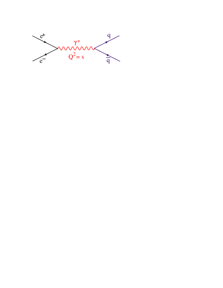
Figure 6: Electron–positron annihilation to lowest order in perturbative QCD

The simplest process in perturbative QCD is electron–positron ($e^{+}e^{-}$) annihilation into hadrons. To lowest order in the electromagnetic ($\alpha_{\rm em}$) and strong ($\alpha_{s}$) coupling constants, this process proceeds as depicted in Fig. 6: the electron and positron annihilate with each other into a time–like virtual photon, with positive virtuality $Q^{2}\equiv-q^{\mu}q_{\mu}=s$ (with $s=(E_{e^{+}}+E_{e^{-}})^{2}$ the total energy squared in the center–of–mass (COM) frame and $q^{\mu}$ the 4–momentum of the photon), which then decays into a quark–antiquark ($q\bar{q}$) pair. This process is ‘hard’ provided the energy is high enough : $\sqrt{s}\gg\Lambda_{{\rm QCD}}$. In a confining theory like QCD, quarks cannot appear in the final state, which must involve only hadrons. Hence, the structure of the final state, as seen by a detector, will be determined by the subsequent evolution of the quark and the antiquark via parton branching (see Fig. 7), with the emerging partons eventually combining into hadrons. Since hadronisation is a non–perturbative process, one may wonder whether it makes any sense at all to use a partonic picture (which is rooted in perturbation theory), even for the early and the intermediate stages of the collision. This is however justified by the separation of time scales in the problem: quantum processes are not instantaneous, rather it takes some time to emit a parton — the more so the softer the parton. Hard processes occur very fast and determine the probability for a scattering to happen, i.e., the total cross–section for $e^{+}e^{-}$ annihilation, which is therefore computable in perturbation theory. The processes responsible for hadronisation involve ‘soft’ quanta with momenta $k\sim\Lambda_{{\rm QCD}}$, hence they occur relatively late and affect only the precise structure of the final state in terms of hadrons, but not the total cross–section.

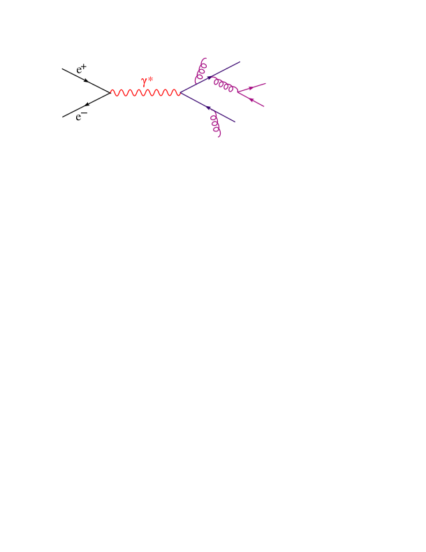
Figure 7: Parton evolution in the final state of $e^{+}e^{-}$ annihilation.

Let us be more specific about these lifetime arguments, as they will play an important role in what follows. One can estimate the duration of a process from the uncertainty principle. The fastest process is the one depicted in Fig. 6 — the $e^{+}e^{-}$ annihilation into a $q\bar{q}$ pair — which in the COM frame lasts for a time $\Delta t_{0}\sim 1/Q=1/\sqrt{s}$. The emitted quark and antiquark are themselves off–shell — each of them carries roughly half of the energy of the virtual photon and half of its virtuality — so they will decay by radiating softer gluons (cf. Fig. 7). The lifetime of a time–like quark (more generally, parton) with 4–momentum $p^{\mu}=(\omega,{\bf p})$ is estimated as

$$\Delta t\,\sim\,\frac{1}{P}\,\gamma\,=\,\frac{\omega}{P^{2}}\,,$$ (2.5)

where the first factor $1/P$ (with $P^{2}=\omega^{2}-p^{2}$ and $p=|{\bf p}|$) is the parton lifetime in its own rest frame and the second factor $\gamma=1/\sqrt{1-v^{2}}={\omega}/{P}$, with $v=p/\omega$, is the Lorentz factor for the relativistic time dilation. This $\Delta t$ can be also interpreted as the formation time of the radiated gluon, and can be alternatively expressed in terms of the kinematics of the latter (see Fig. 7). A simple calculation yields (we assume here that $k_{\parallel}\ll p$)

$$\Delta t\,\sim\,\frac{k_{\parallel}}{k_{\perp}^{2}}\,,$$ (2.6)

where $k_{\parallel}$ and $k_{\perp}$ are the components of the gluon spatial momentum which are parallel and, respectively, perpendicular to the 3–momentum ${\bf p}$ of the parent quark. As anticipated, it takes longer time to emit softer gluons, i.e., gluons with lower transverse momenta $k_{\perp}$. In particular, the hadronisation time is estimated as $t_{\rm hadr}\sim{k_{\parallel}}/\Lambda_{{\rm QCD}}^{2}$ with $k_{\parallel}\lesssim\sqrt{s}$. This means that, at high energy, there exists a parametrically wide interval, namely,

$$\frac{1}{\sqrt{s}}\ <\ t\ <\frac{\sqrt{s}}{\Lambda_{{\rm QCD}}^{2}}\,,$$ (2.7)

during which the effects of confinement can be safely neglected and a parton description applies. Note that the value of the coupling constant did not play any role in this argument, which is rather controlled by the kinematics via the uncertainty principle. On the other hand, the details of the partonic pictures are very different at weak and, respectively, strong coupling, as we shall later discover.

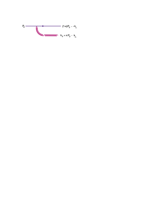
Figure 8: Gluon bremsstrahlung out of a parent quark to lowest order in pQCD.

Sticking to weak coupling for the time being, parton branching is controlled by bremsstrahlung, which to lowest order in pQCD yields the following rate for emitting a gluon out of a parent quark or gluon (see also Fig. 8 and, e.g., [58] for details):

$${\rm d}\mathcal{P}_{\rm Brem}\,\simeq\,\frac{\alpha_{s}C_{R}}{\pi^{2}}\,\frac{{\rm d}^{2}k_{\perp}}{k_{\perp}^{2}}\,\frac{{\rm d}x}{x}\,,$$ (2.8)

where $k_{\perp}$ is the gluon transverse momentum and $x=k_{\parallel}/p$ is the fraction of the parent parton longitudinal momentum which is taken away by the gluon. $C_{R}$ is the Casimir for the SU$(N_{c})$ representation pertinent to the parent parton: $C_{F}=(N_{c}^{2}-1)/N_{c}$ for a quark, or $C_{A}=N_{c}$ for a gluon. In writing Eq. (2.8) we have specialized to $x\ll 1$ since this is the most interesting regime at high energy and weak coupling: as manifest on this equation, the bremsstrahlung favors the emission of relatively soft gluons, with small longitudinal fractions $x\ll 1$ and transverse momenta logarithmically distributed within the range $\Lambda_{{\rm QCD}}<k_{\perp}<k_{\parallel}$, since the corresponding phase–space is large and compensates for the smallness of the coupling:

$$\Lambda_{{\rm QCD}}\,\ll\,k_{\perp}\,\ll\,k_{\parallel}=xp\,\ll\,\sqrt{s}\ \ \Longrightarrow\ \ \mathcal{P}_{\rm soft}\,\sim\,\alpha_{s}(Q^{2})\,\ln^{2}\frac{\sqrt{s}}{\Lambda_{{\rm QCD}}}\,.$$ (2.9)

(The softest among these gluons are responsible for hadronisation.) However, such soft gluons are quasi–collinear with their parents partons, so their emission does not significantly alter the topology of the final state: instead of a pair of bare quarks, the detector will see a pair of well collimated hadronic jets (see Fig. 9 left). Harder emissions leading to multi–jets events (see Fig. 9 right) are possible as well, and actually seen in the experiments, but they are comparatively rare since they occur with a small probability $\mathcal{P}_{\rm hard}\sim\alpha_{s}(Q^{2})\ll 1$ with $Q^{2}=s$. The total cross–section for $e^{+}e^{-}$ annihilation can be computed in pQCD as a series in powers of $\alpha_{s}(s)$, with the different terms in this series roughly corresponding to different numbers of jets in the final state:

$$\sigma(s)\,=\,\sigma_{\rm QED}\,\times\,\big{(}3\sum_{f}e_{f}^{2}\big{)}\left(1\,+\,\frac{\alpha_{s}(s)}{\pi}\,+\,\mathcal{O}{(\alpha_{s}^{2}(s))}\right)\,,$$ (2.10)

where $\sigma_{\rm QED}=4\pi\alpha_{\rm em}^{2}/3s$ is the QED cross–section for $e^{+}e^{-}\to\mu^{+}\mu^{-}$, the factor of $N_{c}=3$ is the number of color degrees of freedom for quarks in SU(3), and $e_{f}$ is the electric charge of the quarks with flavor $f$ (in units of the electron charge $e$). The experimental verification of Eq. (2.10) represents one of the most solidly established tests of pQCD so far.

  

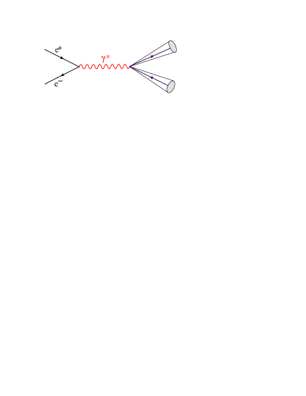
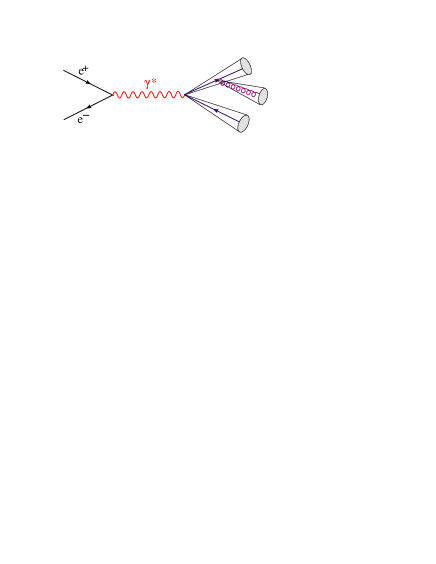
Figure 9: Jet structure in the final state for $e^{+}e^{-}$ annihilation.

  

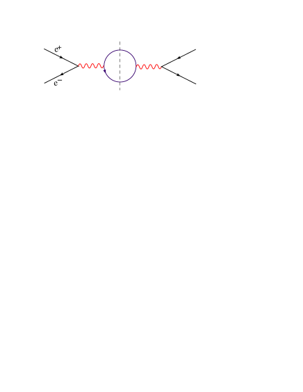
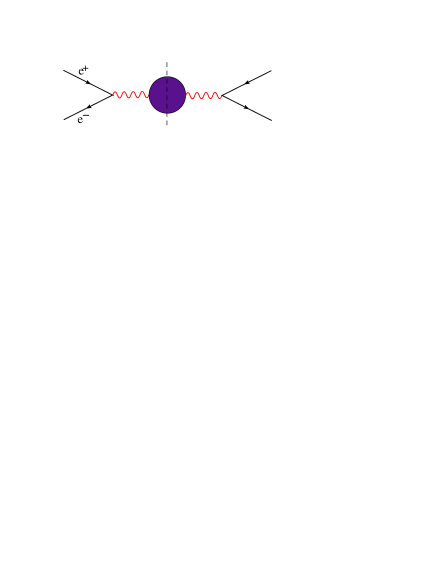
Figure 10: Total cross–section for $e^{+}e^{-}$ annihilation as given by the optical theorem.

To conclude this discussion of $e^{+}e^{-}$ annihilation, let us describe a recipe for computing the corresponding cross–section which goes beyond perturbation theory, and thus also applies in the strong–coupling regime to be considered later on. By the optical theorem, this cross–section can be related to the imaginary part of the forward scattering amplitude $e^{+}e^{-}\to e^{+}e^{-}$. For instance, to lowest order in $\alpha_{s}$, the cross–section for the process $e^{+}e^{-}\to q\bar{q}$ illustrated in Fig. 6 can be expressed as a cut through the one–quark–loop contribution to the forward amplitude, cf. Fig. 10 (left). More generally, the following formula holds to leading order in $\alpha_{\rm em}$ but to all orders in $\alpha_{s}$ :

$$\sigma(e^{+}e^{-})\,=\,\frac{1}{2s}\ \ell^{\mu\nu}\ {\rm Im}\,\Pi_{\mu\nu}(q)\,,$$ (2.11)

where $\ell^{\mu\nu}$ is a leptonic tensor associated with the external electron and positron lines and $\Pi_{\mu\nu}(q)$ is the (retarded) vacuum polarization tensor for the virtual photon, and can in turn be computed as the following current–current correlator in the vacuum (or ‘vacuum polarization tensor’)

$$\Pi_{\mu\nu}(q)\,\equiv\int{\rm d}^{4}x\,{\rm e}^{-iq\cdot x}\,i\theta(x_{0})\,\langle 0\,|\,[J_{\mu}(x),J_{\nu}(0)]\,|\,0\rangle\,,$$ (2.12)

where $J^{\mu}$ is the electromagnetic current density of the quarks :

$$J^{\mu}\,=\,\sum_{f}e_{f}\,\bar{q}_{f}\,\gamma^{\mu}\,q_{f}\,,$$ (2.13)

that is, the operator which couples to the photon: $\mathcal{L}_{\rm int}=eA_{\mu}J^{\mu}$. Current conservation $q^{\mu}\Pi_{\mu\nu}=0$ together with Lorentz symmetry imply that $\Pi_{\mu\nu}$ has only one independent scalar component (recall that $Q^{2}\equiv-q^{\mu}q_{\mu}>0$ and $\eta_{\mu\nu}=(-1,1,1,1)$)

$$\Pi_{\mu\nu}(q)\,=\,\left(\eta_{\mu\nu}+\frac{q_{\mu}q_{\nu}}{Q^{2}}\right)\Pi(Q^{2})\,.$$ (2.14)

Figure 11: Deep inelastic electron–proton scattering: general kinematics.

2.2 Deep inelastic scattering

Another important hadronic process which is mediated by a virtual photon is the deep inelastic scattering (DIS) between a lepton (say, electron) and a hadron (say, the proton), as illustrated in Fig. 11. In DIS, the exchanged photon is space–like: $-q^{\mu}q_{\mu}<0$, and then it is convenient to use the notation $Q^{2}$ for the positive quantity $Q^{2}\equiv q^{\mu}q_{\mu}>0$ (i.e., minus the photon virtuality). The photon couples to the electromagnetic current of the quarks inside the proton. By the optical theorem, the total cross–section $\sigma(ep\to eX)$ can be written similarly to Eq. (2.10), but with the current–current correlator now computed as an expectation value over the proton wavefunction:

$$\Pi_{\mu\nu}(q,P)\,\equiv\int{\rm d}^{4}x\,{\rm e}^{-iq\cdot x}\,i\theta(x_{0})\,\langle P\,|\,[J_{\mu}(x),J_{\nu}(0)]\,|\,P\rangle\,,$$ (2.15)

where the proton state $|\,P\rangle$ is denoted by its 4–momentum $P^{\mu}$. The latter introduces a privileged direction in space, so the tensorial structure of $\Pi_{\mu\nu}$ is more complicated than in the vacuum: it now involves two scalar functions, which both depend upon two kinematical invariants. It is customary to write

$$\Pi_{\mu\nu}(q,P)=\left(\eta_{\mu\nu}-\frac{q_{\mu}q_{\nu}}{Q^{2}}\right)\Pi_{1}(x,Q^{2})+\left(P_{\mu}-q_{\mu}\frac{P\cdot q}{Q^{2}}\right)\left(P_{\nu}-q_{\nu}\frac{P\cdot q}{Q^{2}}\right)\Pi_{2}(x,Q^{2})\,,$$ (2.16)

and express the cross–section in terms of the following structure functions

$$F_{1}(x,Q^{2})\,=\,\frac{1}{2\pi}\,{\rm Im}\,\Pi_{1},\qquad F_{2}(x,Q^{2})\,=\,\frac{-(P\cdot q)}{2\pi}\,{\rm Im}\,\Pi_{2}\,,$$ (2.17)

which are dimensionless. We have here used the following kinematic invariants

$$Q^{2}\,\equiv\,q^{\mu}q_{\mu}\,=\,-q_{0}^{2}+{\bm{q}}^{2}\,\geq\,0,\qquad x\,\equiv\,\frac{Q^{2}}{-2(P\cdot q)}\,=\,\frac{Q^{2}}{s+Q^{2}-M^{2}}\,,$$ (2.18)

where $M$ is the mass of the proton (hence, $P^{2}=-M^{2}$), and $s\equiv-(P+q)^{2}$ is the invariant energy squared of the photon+proton system, and is the same as the invariant mass squared $M_{X}^{2}$ of the hadronic system $X$ produced by the collision, cf. Fig. 11. Note that $M_{X}^{2}\geq M^{2}$ and hence $x\leq 1$. The ‘deep inelastic’ regime corresponds to large virtuality $Q^{2}\gg M^{2}$ (‘hard photon’), and the ‘high energy’ one to small $x$ : $s\gg Q^{2}\,\Longrightarrow\,x\simeq Q^{2}/s\,\ll\,1$.

The kinematical variables in Eq. (2.18) are particularly convenient as they have a direct physical interpretation: they mesure the resolution of the virtual photon as a probe of the internal structure of the proton. More precisely, in a frame in which the proton has a large longitudinal momentum $P\gg M$ (‘infinite momentum frame’, or IMF), the scattering consists in the absorbtion of the virtual photon by a quark excitation which has a longitudinal momentum fraction $k_{z}/P$ equal to $x$ and occupies an area $\sim 1/Q^{2}$ in the transverse plane $(x,y)$ (the plane normal to the collision axis, chosen here to be $z$). This can be understood with reference to Figs. 8, 12, and Eq. (2.6) : a partonic excitation with longitudinal momentum $k_{z}$ and transverse momentum $k_{\perp}$ has a lifetime

$$\Delta t_{\rm part}\,\sim\,\frac{k_{z}}{k_{\perp}^{2}}\,=\,\frac{xP}{k_{\perp}^{2}}\,.$$ (2.19)

For this parton to be ‘seen’ in DIS, it must live longer than the interaction time with the virtual photon, in turn estimated as ($q_{0}$ is the energy of $\gamma^{*}$ in the IMF)

$$\Delta t_{\rm col}\,\sim\,\frac{1}{q_{0}}\,\sim\,\frac{xP}{Q^{2}}\,.$$ (2.20)

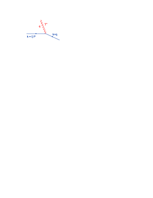
Figure 12: The virtual photon absorbtion by a nearly on–shell quark with longitudinal momentum fraction $\xi$.

This condition requires $k_{\perp}^{2}\lesssim Q^{2}$, which via the uncertainty principle implies that the parton is localized within an area $\gtrsim 1/Q^{2}$. Furthermore, in the IMF, partons are quasi–free and hence nearly on–shell, and their longitudinal momenta are much larger than the transverse ones (they are nearly collinear with the proton). With reference to Fig. 12, these conditions imply

$$k^{2}\,\approx\,0\ \&\ (k+q)^{2}\,\approx\,0 \ \Longrightarrow\ Q^{2}+2\xi P\cdot q\,\approx\,0$$

$$\ \Longrightarrow\ \xi\,=\,\frac{Q^{2}}{-2(P\cdot q)}\,=\,x$$

Note that the choice of the IMF is crucial for the validity of this interpretation: it is only in this frame that the virtual excitations of the proton (quarks and gluons) live long enough — by Lorentz time dilation — to be unambiguously distinguished from vacuum fluctuations with the same quantum numbers and momenta, and to be treated as quasi–free during the comparatively short duration of the scattering with the external probe (here, the virtual photon).

Then the DIS cross–section can be factorized as the elementary cross–section for the photon absorbtion by a quark times a ‘parton distribution function’ which describes the probability to find a quark with longitudinal momentum fraction equal to $x$ and transverse area $1/Q^{2}$. This correspondence is such that the structure function $F_{2}(x,Q^{2})$ introduced in Eq. (2.17) is a direct measure of the quark and antiquark distribution functions:

$$F_{2}(x,Q^{2})\,=\,\sum_{f}e_{f}^{2}\,\big{[}xq_{f}(x,Q^{2})+x\bar{q}_{f}(x,Q^{2})\big{]}\,,$$ (2.21)

where $q_{f}(x,Q^{2})$ is the number of quarks of flavor $f$ with longitudinal momentum fraction $x$ and transverse size $1/Q$. Thus, the experimental measurement of $F_{2}(x,Q^{2})$ gives us a direct access to the phase–space distribution of quarks within the proton wavefunction and in the infinite momentum frame. This gives us furthermore access to the gluon distribution, albeit indirectly, modulo our theoretical understanding of parton evolution.

    

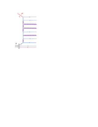
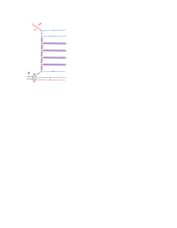
Figure 13: Parton evolution in perturbative QCD. The parton cascade on the right involves only gluons and is a part of the BFKL resummation at small $x$.

Namely, quark and gluons can transform into each other via parton branching, so in general the quark struck by the virtual photon in DIS is a ‘sea’ quark, i.e., a quark from a partonic cascade initiated by one of the valence quarks, as illustrated in Fig. 13. At weak coupling, this branching proceeds through bremsstrahlung and favors an evolution in which the virtuality is strongly increasing when moving up (from the target proton towards the projectile photon) along the cascade. That is, after each individual splitting, the daughter parton emitted in the $t$–channel has either a much larger transverse momentum than its parent parton, or a much smaller longitudinal–momentum fraction (and then it is generally a gluon), or both. This is so since, according to Eq. (2.8), such emissions are favored by the large available phase space, which equals $\ln(Q^{2}/\Lambda_{{\rm QCD}}^{2})$ for the emission of a parton (quark or gluon) with transverse momentum $k_{\perp}\ll Q$ and, respectively, $\ln(1/x)$ for that of a gluon with longitudinal momentum fraction $\xi$ within the range $x\ll\xi\ll 1$. Depending upon the relevant values of $Q^{2}$ and $x$, one can write down evolution equations which resum either powers of $\alpha_{s}\ln Q^{2}$, or of $\alpha_{s}\ln(1/x)$, to all orders; the coefficients in these equations, which represent the elementary splitting probability can be computed as power series in $\alpha_{s}$ starting with the leading–order result in Eq. (2.8). As obvious from the previous considerations, the $Q^{2}$–evolution (as encoded in the DGLAP equation [60]) mixes the quark and gluon distribution functions (see Fig. 13.a), and this allows us to reconstruct the gluon distribution from the $Q^{2}$–dependence of the experimental results for $F_{2}$. The small–$x$ evolution, on the other hand, which is described by the BFKL equation [61] and its non–linear generalizations [53] (see below), involves only gluons and corresponds to resumming ladder diagrams like those in Fig. 13.b in which successive gluons are strongly ordered in $x$.

  

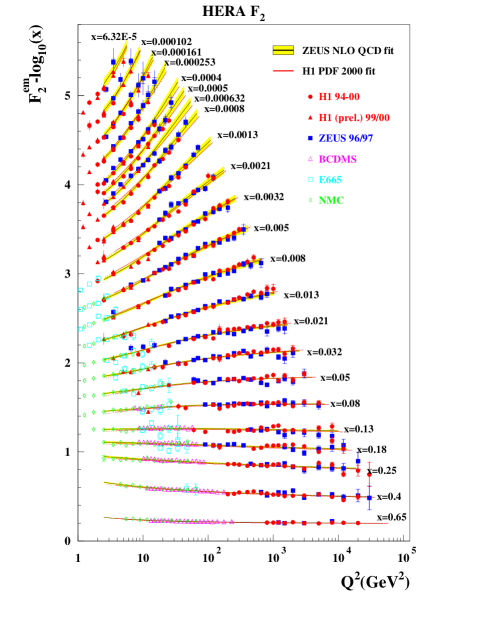
Figure 14: HERA results for $F_{2}$ (combined results from ZEUS and H1) which illustrate the effects of the evolution with increasing $Q^{2}$ for different values of $x$ : $F_{2}$ is increasing with $Q^{2}$ at all the values of $x$ except the very large ones $x\gtrsim 0.2$, where $F_{2}$ is decreasing.

Here, we shall not discuss the perturbative evolution in more detail, but merely emphasize some features which are interesting for comparison with the situation at strong coupling, to be described later on. First note that the parton lifetime, cf. Eq. (2.19), is strongly decreasing when moving up along the cascade (for both the $Q^{2}$ and the small–$x$ evolutions), so that the cascade is frozen — the parton distribution is fixed within it — during the relatively short duration of the collision with $\gamma^{*}$, cf. Eq. (2.20), which is the same as the lifetime of the struck quark. Second, after each splitting, the energy of the parent parton gets divided among the two daughter ones, so we expect the evolution to increase the number of partons at small values of $x$ and decrease that at larger values. Moreover, the gluon distribution should rise faster with decreasing $x$, so the small–$x$ partons should be predominantly gluons. These expectations are indeed confirmed by the experimental results at HERA displayed in Figs. 14 and 15 [62] (and Refs. therein).

  

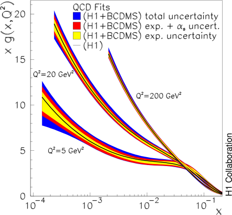
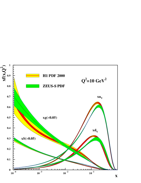
Figure 15: Parton distributions extracted from combined fits to the H1 and ZEUS data at HERA, which illustrate the evolution with decreasing $x$ at fixed $Q^{2}$. Left: the rise in the gluon distribution. Right: the $1/x$–evolution of the gluon, sea quark, and valence quark distributions for $Q^{2}=10$ GeV² (note that the gluon and sea quark distributions have been reduced by a factor of 20 to fit inside the figure).

But although they are less numerous, the few partons remaining at larger values of $x$ do still carry most of the total energy of the proton, and that even for very large $Q^{2}$. This is so since the dominant evolution is such that the daughter gluon takes away only a small fraction of the longitudinal momentum of its parent parton, so the latter ‘survives’ (as one of the $s$–channel partons in the cascades in Fig. 13) with a relatively large momentum. To see this more quantitatively, consider the following ‘energy sum–rule’, which is the condition that the ensemble of partons (quarks, antiquarks, and gluons) which exist on a given resolution scale $Q^{2}$ carry the totality of the proton longitudinal momentum:

$$\int_{0}^{1}{\rm d}x\,x\big{[}q(x,Q^{2})+{\bar{q}}(x,Q^{2})+g(x,Q^{2})\big{]}\,=\,1\,.$$ (2.22)

The HERA data show that the ‘gluon distribution’ $xg(x,Q^{2})$ rises with $1/x$ roughly like $xg(x,Q^{2})\sim 1/x^{\omega}$ for $x\leq 0.01$, but the exponent $\omega$ is small enough, namely $\omega=0.2\div 0.3$ (it slowly varies with $Q^{2}$), for the integral in Eq. (2.22) to be dominated by large values $x\sim 1$. This value $\omega=0.2\div 0.3$ is indeed consistent with predictions of the QCD evolution equations at next–to–leading–order (NLO) accuracy.

However, such a power increase with $1/x$ cannot continue forever, i.e., not up to arbitrarily high energies, since this would enter in conflict with the unitarity constraint for DIS and other hadronic processes. For instance, the cross–section for the virtual photon absorbtion by the proton in DIS is related to $F_{2}$ :

$$\sigma_{\gamma^{*}p}(x,Q^{2})\,=\,\frac{4\pi^{2}\alpha_{\rm em}}{Q^{2}}\,F_{2}(x,Q^{2})\,.$$ (2.23)

In the high–energy limit $x\to 0$ we expect this cross–section to grow, at most, like a power of $\ln(1/x)$; this is Froissart bound and is a consequence of the unitarity of the $S$–matrix. (A similar bound holds for the $pp$ collisions to be studied at LHC.) There are also physical arguments which are supported by explicit calculations within pQCD and which are telling us what should be the physical mechanism responsible for taming this growth: this is gluon saturation. With increasing energy, the gluon density increases as well and eventually it becomes so high that the gluon start interacting with each other — meaning that the evolution starts to be non–linear — and these interactions limit the further growth of the gluon occupation number.

To understand the relevance of the occupation number — a concept that will be important at strong coupling as well — notice that, in order to interact with each other, the gluons must overlap, meaning that not only their number, but also their (longitudinal and transverse) sizes, should be large enough. At high–energy, the proton is Lorentz contracted — it looks to the virtual photon like a pancake — so all the partons within a longitudinal tube at a given impact parameter can interact with the photon and also with each other. This argument must be corrected for the uncertainty principle, but it is essentially correct: the small–$x$ partons, with longitudinal momenta $k_{z}\simeq xP$, are delocalized in $z$ over a distance $\Delta z\sim 1/xP$, which is of the same order as the longitudinal wavelength of the virtual photon. Incidentally, this argument also shows that the longitudinal phase–space for DIS at high energy is measured by the rapidity $Y\equiv\ln(1/x)\simeq\ln(s/Q^{2})$ :

$$\Delta k_{z}\,\Delta z\,\sim\,\frac{\Delta(xP)}{xP}\,\sim\,\frac{\Delta x}{x}\,\sim\,\Delta Y\,.$$ (2.24)

Indeed, the parton distributions are defined as the number of partons per unit rapidity ; e.g.,

$$xg(x,Q^{2})\,\equiv\,x\,\frac{{\rm d}N_{g}}{{\rm d}x}(Q^{2})\,=\,\int{\rm d}^{2}b_{\perp}\ \int^{Q}\!\!{\rm d}^{2}k_{\perp}\ \frac{{\rm d}N_{g}}{{\rm d}Y{\rm d}^{2}b_{\perp}{\rm d}^{2}k_{\perp}}\,,$$ (2.25)

where the first integral runs over all impact parameters within the proton transverse area and the second one over all the transverse momenta up to $Q$ (cf. the discussion after Eq. (2.20)).

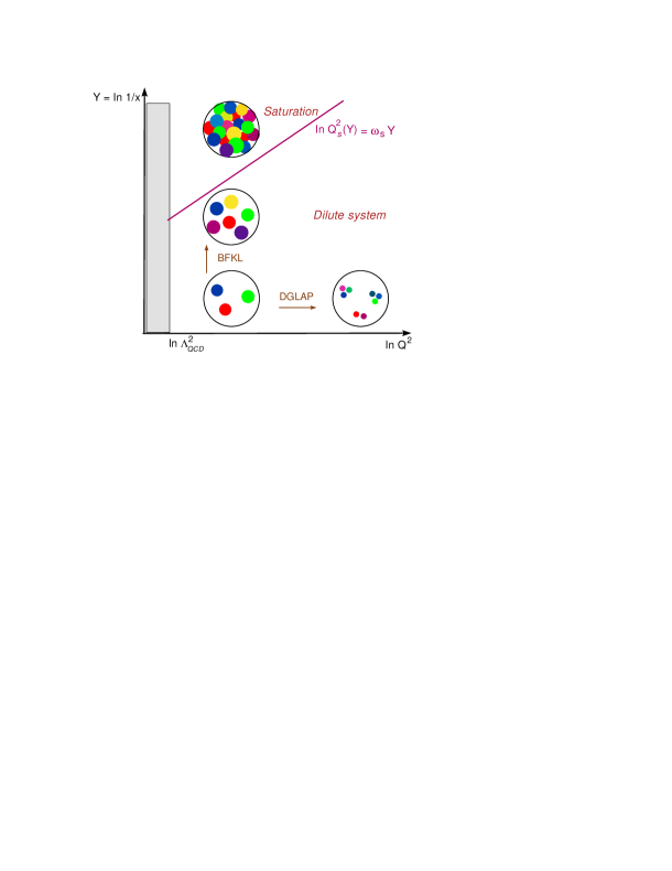
Figure 16: The phase–space for parton evolution in the kinematical variables appropriate for DIS ($\ln Q^{2}$ and $Y=\ln 1/x$), which illustrates the distribution of partons (shown as colored blobs with area $\sim 1/Q^{2}$) within the proton disk, and the saturation line $\ln Q^{2}_{s}(Y)=\omega_{s}Y$.

Consider now the gluon overlap in the two–dimensional transverse space. As illustrated in Fig. 16, when $Q^{2}$ is high, the gluons form a dilute system (although they are relatively numerous) because each of them occupies only a small area $\sim 1/Q^{2}$. But when decreasing $x$ at fixed $Q^{2}$, one emits more and more gluons having (almost) the same area, so these gluons will eventually start overlapping. We see that, what controls the gluon interactions with each other, is not their number density ${xg(x,Q^{2})}/{\pi R^{2}}$ ($R$ is the proton radius), but rather their occupation number

$$n_{g}(Y,b_{\perp},k_{\perp})\,\equiv\,\frac{(2\pi)^{3}}{2(N_{c}^{2}-1)}\,\,\frac{{\rm d}N_{g}}{{\rm d}Y\,{\rm d}^{2}b_{\perp}{\rm d}^{2}k_{\perp}}\,\sim\,\frac{1}{Q^{2}}\times\frac{xg(x,Q^{2})}{\pi R^{2}(N_{c}^{2}-1)}\,.$$ (2.26)

As shown by the last estimate, $n_{g}$ measures the ‘fraction’ of the proton area which is covered with gluons of a given color. This ‘fraction’ can be bigger than one since the gluons can overlap with each other. In fact, at weak coupling, the gluon interactions become an effect of $\mathcal{O}{(1)}$ when $n_{g}\sim 1/(\alpha_{s}N_{c})\sim 1/\lambda$, since in that case the overlap is strong enough to compensate for the smallness of the coupling. This condition defines a critical line in the kinematical plane $(x,Q^{2})$ — the saturation line — which separates between a dilute region where $n_{g}\ll 1/\lambda$ and a dense region where the occupation number saturates at a value $n_{g}\sim\mathcal{O}{(1/\lambda)}$ (see Fig. 16). One can solve this condition for $Q^{2}$ and thus deduce the saturation momentum

$$Q^{2}_{s}(x)\,\sim\,{\lambda}\,\frac{xg(x,Q^{2}_{s})}{R^{2}(N_{c}^{2}-1)}\,\,\sim\,\,\frac{1}{x^{\omega}}\,,$$ (2.27)

which is the value of the transverse momentum around which non–linear effects become important for a given value of $x$. Alternatively, this is the photon virtuality at which unitarity corrections become important in DIS. As shown in Eq. (2.27), $Q^{2}_{s}(x)$ rises with $1/x$ roughly like the gluon distribution, i.e., as a power $1/x^{\omega}$ with ${\omega}\simeq 0.2\div 0.3$ from fits to the HERA data. (In logarithmic coordinates $(Y,\ln Q^{2})$, this yields a saturation line which is a straight line, as shown in Fig. 16.) Thus, with increasing energy, the saturation region extends to higher and higher values of $Q^{2}$, i.e., to smaller and smaller gluons.

These conclusions are supported by more refined analyses within pQCD, which succeeded in resumming the non–linear effects associated with gluon saturation within the evolution equations at high energy. This led to non–linear generalizations of the BFKL equation — the functional JIMWLK equation and its mean–field (or large–$N_{c}$) approximation known as BK — which describe the transition towards saturation with increasing energy and thus permit the calculation of the saturation line (see the review papers [53] and references therein). So far, the full non–linear equations are known only to leading–order accuracy at weak coupling, but the asymptotic form of the saturation line at high energy is also known to NLO accuracy [63]. Interestingly, such analyses confirm the power–law behaviour $Q^{2}_{s}(x)\sim{1}/{x^{\omega_{s}}}$ (at least, as an approximation valid in a limited range in $Y$), but the value of the saturation exponent $\omega_{s}$ is strongly reduced by NLO corrections: one finds $\omega_{s}\simeq 4.88(\alpha_{s}N_{c}/\pi)\simeq 0.12\lambda$ at LO (which would yield $\omega_{s}\sim 1$ for $\alpha_{s}=0.2$ and $N_{c}=3$), but $\omega_{s}\simeq 0.3$ at NLO. Note that this NLO value is roughly consistent with the experimental results at HERA, thus suggesting that the (unknown) corrections of higher order should be rather small. In fact, a substantial fraction of the NLO corrections comes from the running of the coupling [63].

3 Current–current correlator from AdS/CFT: General formalism

With this section, we begin the study of the main problem of interest tous here, which is the propagation of a high–energy abelian current through a strongly coupled plasma at temperature $T$. As mentioned in the Introduction, our plasma will not be that of QCD, but rather the one described by the maximally supersymmetric ${\mathcal{N}}=4$ Yang–Mills theory, which is conformally invariant (so, in particular, the coupling is fixed), and for which the AdS/CFT correspondence is most firmly established. Since we shall not perform calculations directly in the gauge theory (but only in the ‘dual’ superstring theory), there is no need to exhibit the Lagrangian of ${\mathcal{N}}=4$ SYM. (This can be found in the textbooks listed in the References [54, 55].) For our purposes, it suffices to recall that this Lagrangian involves 3 types of massless fields — gluons, 4 Majorana fermions, and 6 real scalars — which all transform under the adjoint representation of the colour group SU$(N_{c})$. Besides the Lagrangian has a global SU(4) ${\mathcal{R}}$–symmetry (that is, a symmetry which does not commute with the supersymmetry generators), under which the gluons are neutral, the four fermions transform as a ${\bf 4}$ or $\bar{\bf 4}$ (depending upon their chirality), and the six scalars transform as a ${\bf 6}$. This global symmetry is interesting for our purposes as it allows one to introduce an analog of the electromagnetism: to that aim, we shall pick one of the U(1) subgroups of SU(4) and gauge it, that is, replace the ordinary derivatives by covariant derivatives: $\partial_{\mu}\to\partial_{\mu}-iet^{a_{0}}_{R}A_{\mu}^{a_{0}}$ where $a_{0}$ is the SU(4)–index of the chosen U(1) subgroup, $t^{a_{0}}_{R}$ is the respective generator in the appropriate representation, and $A_{\mu}^{a_{0}}$ is an Abelian gauge field endowed with the standard, Maxwell–like, kinetic term in the action. Furthermore, $e$ is the analog of the electric charge, that we shall take to be arbitrarily small. In the subsequent formulae, the charge $e$ and the index $a_{0}$ will be always omitted. Associated to $A_{\mu}^{a_{0}}\equiv A_{\mu}$ there is a conserved ‘electric current’ $J^{\mu}$, obtained by rewriting the interaction terms in the action as $A_{\mu}J^{\mu}$. This current is built with selected fermionic and scalar fields (see e.g. [77] for an explicit construction). We shall refer to it as the ‘${\mathcal{R}}$–current’.

The problem that we shall consider will be the scattering between this ${\mathcal{R}}$–current and the ${\mathcal{N}}=4$ SYM plasma in the high–energy regime (the kinematics will be shortly specified) and in the strong t’ Hooft coupling limit taken as

$$N_{c}\,\to\,\infty\quad\mbox{and}\quad\lambda\equiv g^{2}N_{c}\,\to\,\infty\quad\mbox{with}\quad g^{2}\,\ll\,1.$$ (3.28)

That is, $N_{c}$ is taken to be arbitrarily large whereas the gauge coupling $g$ is fixed and small. This limit is convenient for applications of the AdS/CFT correspondence, as we now explain.

The AdS/CFT conjecture establishes a correspondence, or ‘duality’, between the ${\mathcal{N}}=4$ SYM theory (the ‘Conformal Field Theory’) with arbitrary values for the parameters $g$ and $N_{c}$ and the type IIB superstring theory living in a $D=10$ curved space–time which is $AdS_{5}\times S^{5}$ (hence, the ‘AdS’). This duality means that the background geometry for the string theory corresponds to the vacuum of the gauge theory, and that all the observables (like gauge–covariant correlation functions) in one description can be equivalently calculated — after appropriate identifications — in the other description. The duality extends to finite temperature by adding a ‘black hole’ to $AdS_{5}$. One thus obtains the $AdS_{5}\times S^{5}$–Schwarzschild metric, for which a common parametrization reads

$${\rm d}s^{2}=\frac{r^{2}}{R^{2}}(-f(r){\rm d}t^{2}+{\rm d}\bm{x}^{2})+\frac{R^{2}}{r^{2}f(r)}{\rm d}r^{2}+R^{2}{\rm d}\Omega_{5}^{2}\,,$$ (3.29)

where $t$ and $\bm{x}=(x,y,z)$ are the time and spatial coordinates of the physical Minkowski world, $r$ (with $0\leq r<\infty$) is the radial coordinate on $AdS_{5}$ (or ‘5th dimension’), and ${\rm d}\Omega^{2}_{5}$ is the angular measure on $S^{5}$. Furthermore, $R$ is the common radius of $AdS_{5}$ and $S^{5}$, and

$$f(r)\,=\,1-\frac{r_{0}^{4}}{r^{4}}\,=\,1-u^{2}\,=\,1-\frac{\chi^{4}}{\chi_{0}^{4}}\,,$$ (3.30)

where $r_{0}$ is the Black Hole (BH) horizon and is related to its temperature $T$ (the same as for the ${\mathcal{N}}=4$ SYM plasma) via $r_{0}=\pi R^{2}T$. (Note that this BH is homogeneous in the four physical dimensions but has an horizon in the fifth dimension which encloses the real singularity at $r=0$.) When $r\to\infty$, $f(r)\to 1$ and ${\rm d}s^{2}\propto(-{\rm d}t^{2}+{\rm d}\bm{x}^{2})$ is conformal to the flat Minkowski metric. Hence, the boundary of $AdS_{5}$ at $r\to\infty$ will be referred to as the ‘Minkowski boundary’. In fact, we have $f(r)\approx 1$ whenever $r\gg r_{0}$, so far away from the horizon the geometry is $AdS_{5}\times S^{5}$. As shown in Eq. (3.30), some other radial coordinates will be also used in what follows: these are defined as $u\equiv(r_{0}/r)^{2}$ and $\chi\equiv R^{2}/r=\sqrt{u}/(\pi T)$, and in terms of them the Minkowski boundary lies at $u=\chi=0$ and the BH horizon at $u_{0}=1$ and, respectively, $\chi_{0}=1/\pi T$.

Besides $R$, the superstring theory involves two more parameters, the (dimensionless) string coupling constant $g_{s}$ and the string length $\ell_{s}$, which is the characteristic scale on which the string structure (as opposed to a point–like particle) can be resolved, and is related to the Planck length in ten dimensions by $\ell_{\rm P}=g_{s}^{1/4}\ell_{s}$. The AdS/CFT correspondence makes the following identification between the free parameters of the two dual descriptions:

$$4\pi g_{s}\,=\,g^{2}\,,\qquad(R/\ell_{s})^{4}\,=\,g^{2}N_{c}\,\equiv\,\lambda\,.$$ (3.31)

The first relation tells us that when the Yang–Mills coupling $g^{2}$ is small, so is also the string coupling, hence one can neglect quantum corrections (string loops) on the string theory side. The second relation shows that when $\lambda$ is large, the geometry of the string theory is weakly curved, so that the massive string excitations (with mass $m\sim R/\ell_{s}^{2}$) can be reliably decoupled from the low–energies ones, and then the superstring theory reduces to type IIB supergravity. Hence, when we have both $g^{2}\ll 1$ and $\lambda\to\infty$ — this corresponds to the strong coupling limit of the ${\mathcal{N}}=4$ SYM theory in the sense of Eq. (3.28) —, the dual superstring theory reduces to classical supergravity in ten dimensions. After also performing a Kaluza–Klein reduction around $S^{5}$ and keeping only the lowest harmonics, one finally obtains a classical theory in five dimensions which involves massless fields, among which the (5-dimensional) graviton, the dilaton, and a SO(6) $\simeq$ SU(4) non–Abelian gauge field. The quantum correlation functions in the strongly coupled CFT can now be computed from solutions to the classical equations of motion for these massless fields with appropriate boundary conditions.

In what follows, we shall describe this calculation for the problem of interest here, namely the correlation functions of the ${\mathcal{R}}$–current $J_{\mu}$. Let $Z_{4D}[A_{\mu}]$ denote the respective generating functional in the 4–dimensional gauge theory ($A^{\mu}(x)$ is a ‘dummy’ source field for $J_{\mu}$). Within AdS/CFT, the current $J_{\mu}$ is viewed as a perturbation of the supergravity fields acting at the Minkowski boundary ($r\to\infty$, or $u=0$). Recall that $J_{\mu}$ carries a hidden SU(4)–group index $a_{0}$, in addition to the manifest 4D vector index $\mu$. Thus, by covariance, it is natural that this current induces a non–zero expectation value for the respective component $A_{m}^{a_{0}}\equiv A_{m}$ of the SO(6) vector field in 5D supergravity. (We use $m,\,n,\,p,...$ to denote vector indices on $AdS_{5}$: $m=0,1,2,3,u$.) For more clarity, let us temporarily denote by $A^{m}_{\rm cl}$ the solution to the supergravity equations of motion obeying the appropriate boundary conditions, that will be shortly specified. In the strong coupling limit of Eq. (3.28), $Z_{4D}[A_{\mu}]$ can be computed as

$$Z_{4D}[A_{\mu}]\,\equiv\,\big{\langle}{\rm e}^{i\int{\rm d}^{4}xJ_{\mu}A^{\mu}}\big{\rangle}\ =\ {\rm e}^{iS_{\rm SUGRA}[A_{\rm cl}]}\,,$$ (3.32)

where $S_{\rm SUGRA}[A_{\rm cl}]$ is the supergravity action evaluated with the classical solution $A^{m}_{\rm cl}$ which in turn obeys the boundary condition (BC)

$$A_{\mu}^{\rm cl}(x,u=0)=A_{\mu}(x),\qquad A_{u}^{\rm cl}(x,u=0)=0\,,$$ (3.33)

and hence it is a functional of the 4D ‘source’ field $A_{\mu}(x)$. The classical EOM being second order differential equations, a second boundary condition is needed to uniquely specify their solutions. As a general rule, we shall require the solution to be regular everywhere in the ‘bulk’ (i.e., away from the Minkowsky boundary) of $AdS_{5}$. As we shall see, however, this condition is not always sufficient, especially at finite temperature. Whenever the solution involves modes which are propagating in the radial direction, and which in general can either approach towards the boundary (‘incoming’), or move away from it (‘outgoing’), we shall require the physical solution to involve outgoing modes alone. In the finite $T$ case, this can be physically understood as the condition that the modes be fully absorbed by the BH, without reflecting wave. More generally, at both zero and non–zero $T$, this ‘outgoing wave’ prescription generates the retarded current–current correlator [64], which at finite $T$ is defined as

$$\Pi_{\mu\nu}(q)\,\equiv\,i\int{\rm d}^{4}x\,{\rm e}^{-iq\cdot x}\,\theta(x_{0})\,\langle[J_{\mu}(x),J_{\nu}(0)]\rangle_{T}\,,$$ (3.34)

with the brackets denoting the thermal expectation value. Note that, in order to compute $\Pi_{\mu\nu}$, it is sufficient to know the classical action to quadratic order in the source field $A_{\mu}$, meaning that we can take the latter (and hence the field $A^{m}_{\rm cl}$ induced in the bulk) to be arbitrarily weak. Accordingly, we need the supergravity action only to quadratic order in $A^{m}$; not surprisingly, this is the same as the Maxwell action in the $AdS_{5}\times S^{5}$–Schwarzschild background geometry:

$$S\,=\,-\frac{N^{2}_{c}}{64\pi^{2}R}\int{\rm d}^{4}x{\rm d}u\sqrt{-g}\,g^{mp}g^{nq}\,F_{mn}F_{pq}\,,$$ (3.35)

where $F_{mn}=\partial_{m}A_{n}-\partial_{n}A_{m}$, $\partial_{m}=\partial/\partial x^{m}$ with $x^{m}=(t,\bm{x},u)$, $g=\det(g_{mn})$ is the determinant of the matrix made with the covariant components of the metric on $AdS_{5}$, cf. Eq. (3.29), and $g^{mn}$ are the respective contravariant components, as obtained by inverting the matrix $(g_{mn})$. The classical EOM generated by (3.35) are Maxwell equations in a curved space–time:

$$\partial_{m}\big{(}\sqrt{-g}g^{mp}g^{nq}F_{pq})\,=\,0\,.$$ (3.36)

We shall work in the gauge $A_{u}=0$ (which is consistent with the BC in Eq. (3.33)) and choose the incoming perturbation as a plane wave propagating in the $z$ direction, with longitudinal momentum $k$ and energy $\omega$ in the plasma rest frame: that is, our source field reads $A_{\mu}(x)=A_{\mu}^{(0)}{\rm e}^{-i\omega t+ikz}$. Eq. (3.36) being linear, the solution $A^{\rm cl}_{\mu}$ (that we shall simply denote as $A_{\mu}$ from now on, and refer to as the “Maxwell wave”) preserves this plane–wave structure in the Minkowski directions

$$A_{\mu}(t,\bm{x},u)\,=\,{\rm e}^{-i\omega t+ikz}\,A_{\mu}(u)\,,$$ (3.37)

so the only non–trivial dependence is that upon $u$. This is determined by the following equations, as obtained from Eq. (3.36) (below, $i=1,2$) :

$$\varpi A^{\prime}_{0}+\kappa fA_{3}^{\prime}\,=\,0$$ (3.38)

$$A_{i}^{\prime\prime}+\frac{f^{\prime}}{f}A_{i}^{\prime}+\frac{\varpi^{2}-\kappa^{2}f}{uf^{2}}A_{i}\,=\,0$$ (3.39)

$$A_{0}^{\prime\prime}-\frac{1}{uf}(\kappa^{2}A_{0}+\varpi kA_{3})\,=\,0$$ (3.40)

where a prime on a field indicates a $u$–derivative and we have introduced dimensionless, energy and longitudinal momentum, variables, defined as

$$\varpi\equiv\frac{\omega}{2\pi T}\,,\qquad\kappa\equiv\frac{k}{2\pi T}\,.$$ (3.41)

Denoting $a(u)\equiv A_{0}^{\prime}(u)$, Eqs. (3.38) and (3.40) can be combined to give

$$a^{\prime\prime}+\,\frac{(uf)^{\prime}}{uf}\,a^{\prime}+\,\frac{\varpi^{2}-\kappa^{2}f}{uf^{2}}\,a\,=\,0\,.$$ (3.42)

The boundary conditions (3.33) together with Eq. (3.40) imply

$$A_{\mu}(u=0)=A_{\mu}^{(0)}\ \Longrightarrow\ \lim_{u\to 0}\big{[}ua^{\prime}(u)\big{]}\,=\,\kappa^{2}A_{0}^{(0)}+\varpi\kappa A_{3}^{(0)}\,.$$ (3.43)

The field $a$ describes a longitudinal wave, while $A_{1}$ and $A_{2}$ are transverse wave.

Because of the assumed plane wave structure, the action density in Eq. (3.35) is homogeneous in the physical Minkowski directions, so the corresponding integrations simply yield the volume of the 4D space–time: $S=\int{\rm d}^{4}x\,\mathcal{S}=\Delta V\,\Delta t\,\mathcal{S}$. When evaluated on the classical solution, the action density $\mathcal{S}$ is quadratic in the boundary values $A_{\mu}^{(0)}$ and yields the retarded polarization tensor via differentiation (with $q^{\mu}=(\omega,0,0,k)$):

$$\Pi_{\mu\nu}(q)\,=\,\frac{\partial^{2}\mathcal{S}}{\partial A_{\mu}^{(0)}\partial A_{\nu}^{(0)}}\,.$$ (3.44)

To that aim, it is useful to notice that the classical action density can be fully expressed in terms of the values of the field $\tilde{A}_{\mu}(u)$ and of its first derivative at $u=0$ :

$$\mathcal{S}=\,\frac{N^{2}_{c}T^{2}}{16}\,\Big{[}-A_{0}\partial_{u}A_{0}^{*}+fA_{3}\partial_{u}A_{3}^{*}+fA_{i}\partial_{u}A_{i}^{*}\Big{]}_{u=0}\,.$$ (3.45)

(The appearance of the factor $T^{2}$ in front of $\mathcal{S}$ is merely a consequence of our definition of the variable $u$, which scales like $T^{2}$, so $\partial_{u}\sim 1/T^{2}$.) Eq. (3.45) follows from (3.35) after using the EOM (3.36) to perform an integration by parts over $u$ and dropping the contribution from the upper limit $u=1$ (i.e., from the BH horizon), in accordance with the prescription in Ref. [64, 66]. A star on a field denotes complex conjugation: the classical solutions develop an imaginary part (in spite of obeying equations of motion with real coefficients) because of the outgoing–wave condition at large $u$. Via Eq. (3.44), this introduces an imaginary part in $\Pi_{\mu\nu}(q)$ which physically describes the dissipation of the current in the original gauge theory. In fact, the imaginary part of the expression within the square brackets in Eq. (3.45) is independent of $u$ and hence it can be evaluated at any $u$ [64].

Eqs. (3.38)–(3.45) encode various physical phenomena depending upon the kinematics : When $\omega$ and $k$ are relatively small, $\omega,\,k\ll T$, with moreover $\omega\ll k$, these equations describe the diffusion of the $\mathcal{R}$–charge in the strongly–coupled plasma and can be used to compute the respective transport coefficient; this has been studied at length in Refs. [65, 64, 66, 67, 14]. When $\omega=k$, they describe the photon emission from the plasma (for $\mathcal{R}$–photons, of course); this has been studied in Ref. [77] for the case $\omega,\,k\sim T$. When $\omega$ and $k$ are large compared to $T$, the equations describe the high–energy scattering between the $\mathcal{R}$–current (or the virtual $\mathcal{R}$–photon) and the plasma. This is the problem addressed in Refs. [30, 31] and to which we shall devote our attention in what follows. More precisely, we are interested in ‘hard probes’, so we shall choose a current with relatively high virtuality : $Q^{2}\equiv{|\omega^{2}-k^{2}|}\gg T^{2}$, which probes the structure of the plasma on distances much shorter than the thermal wavelength $1/T$. For a space–like current ($\omega<k$), this set–up describes DIS, whereas for a time–like current ($\omega>k$), it describes the current decay into partons and their subsequent evolution in the plasma. In what follows, we shall mostly assume the high–energy kinematics $\omega\sim k\gg Q$, since this is the most interesting one for our purposes.

To conclude this section, let us present a different form of the equations of motion, obtained after some change of variables, which will be useful later on. For definiteness, we concentrate on the longitudinal mode, and denote

$$a(u)\,\equiv\,\frac{1}{(2\pi T)^{2}}\,\frac{\psi(\chi)}{\sqrt{\chi}}\,.$$ (3.46)

(Recall that $\chi\equiv{R^{2}}/{r}={\sqrt{u}}/{\pi T}$.) Then Eq. (3.42) becomes

$$\psi^{\prime\prime}\,+\,\frac{1}{4\chi^{2}}\,\psi\,+\,\frac{\omega^{2}-k^{2}f}{f^{2}}\,\psi\,+\,\frac{f^{\prime}}{f}\bigg{(}\psi^{\prime}-\frac{1}{\chi}\,\psi\bigg{)}\,=\,0\,,$$ (3.47)

where the prime now denotes differentiation w.r.t. $\chi$. This form of the equation is interesting since the last term, proportional to $f^{\prime}$, can be neglected in all cases of interest, as we shall later argue. If so, then the above equation becomes formally identical to the Schrödinger equation for a non–relativistic particle with mass $k$ which is in a stationary state with zero energy:

$$-\frac{1}{2k}\,\frac{\partial^{2}\psi}{\partial\chi^{2}}\,+\,V(\chi)\psi\,=\,E\psi\,,\quad\mbox{with}\quad V(\chi)=-\frac{1}{8k\chi^{2}}-\frac{\omega^{2}-k^{2}f}{2kf^{2}}\quad\mbox{and}\quad E=0\,.$$ (3.48)

This representation will allow us to use the intuition developed with the Schrödinger equation for studies of the Maxwell wave propagating in the $AdS_{5}$ geometry. A time–dependent generalization of this equation will be also useful. Namely, assume that, instead of being a pure plane–wave, the incoming perturbation, and thus the induced field $A_{\mu}$, are wave–packets in energy peaked around $\omega$. The corresponding equations of motion are obtained by replacing

$$-\omega^{2}\,\longrightarrow\,\frac{\partial^{2}}{\partial t^{2}}\,\approx\,-\omega^{2}-2i\omega\frac{\partial}{\partial t}$$ (3.49)

in equations like Eq. (3.42). (The approximate equality above holds since the additional time dependence on top of the phase ${\rm e}^{-i\omega t}$ is weak.) Then Eq. (3.48) is replaced by the time–dependent version of the Schrödinger equation, which reads (in the high–energy kinematics $\omega\sim k\gg Q$)

$$i\frac{\partial\psi}{\partial t}\,=\,-\frac{1}{2k}\,\frac{\partial^{2}\psi}{\partial\chi^{2}}\,+\,V(\chi)\psi\,.$$ (3.50)

In what follows, it will be useful to consider solutions to this equation with the initial condition that, at $t=0$, the field $\psi(t=0,\chi)$ is localized near the Minkowski boundary at $\chi=0$. Physically, this corresponds to a point–like current, as we shall see.

4 The vacuum case as a warm up

Let us first consider the zero–temperature case, i.e. the propagation of the ${\mathcal{R}}$–current through the vacuum of the ${\mathcal{N}}=4$ SYM theory at infinite ’t Hooft coupling (cf. Eq. (3.28)). Although the corresponding result for $\Pi_{\mu\nu}$ is a priori known, for reasons to be later explained, it is nevertheless interesting to go through the calculations and explicitly deduce this result, in order to get acquainted with the AdS/CFT formalism in a relatively simple set–up. Moreover, as explained in Sect. 2, this result covers an interesting physical problem: via Eq. (2.10), it provides the total cross–section for the analog of electron–positron annihilation at strong coupling. The most interesting conclusion which will emerge from the present discussion is that the AdS/CFT calculation is not merely a ‘black box’: by using its results together with physical intuition and general arguments (like the uncertainty principle), one can develop some physical understanding of the underlying process and of the structure of the final state. That is, one get some physical insight into the ‘blob’ on the photon line in the right–hand figure in Fig. 10.

In the dual, supergravity, calculation the Maxwell wave propagates through pure $AdS_{5}$ (no black hole), according to equations which are obtained by letting $f\to 1$ in the equations in the previous section. With $f=1$, Eqs. (3.38)–(3.42), or (3.47), depend upon $\omega$ and $k$ only via the Lorentz–invariant combination $\omega^{2}-k^{2}$, which defines the virtuality of the ${\mathcal{R}}$–current: $q^{\mu}q_{\mu}=k^{2}-\omega^{2}$. This is as it should, since there is no privileged frame at $T=0$. Then current conservation implies that $\Pi_{\mu\nu}(q)$ has the transverse structure displayed in Eq. (2.14), i.e.

$$\Pi_{\mu\nu}(q)=\left(\eta_{\mu\nu}-\frac{q_{\mu}q_{\nu}}{q^{2}}\right)\Pi(q^{2})\,\qquad\mbox{(vacuum)}\,.$$ (4.51)

The scalar function $\Pi(q^{2})$ can be computed from a study of the longitudinal sector alone, that is, by solving the vacuum version of Eq. (3.47), which reads

$$-\frac{1}{2k}\,\psi^{\prime\prime}\,+\,\left(-\frac{1}{8k\chi^{2}}\,\pm\,\frac{Q^{2}}{2k}\right)\psi\,=\,0\,.$$ (4.52)

where we recall that $Q^{2}\equiv|k^{2}-\omega^{2}|$ and the plus (minus) sign in front of $Q^{2}/2k$ corresponds to a space–like (time–like) current. As anticipated, this is of the Schrödinger type, with the potential exhibited in Fig. 17. Already this figure is telling us a lot about the dynamics: (i) in the space–like case, there is a potential barrier with height $\sim Q^{2}/k$, so the wave can penetrate only in the ‘classically allowed region’ on the left of the barrier, at $\chi\lesssim 1/Q$; (ii) in the time–like case, there is no such barrier, so the wave can penetrate up to arbitrarily large values of $\chi$, where it moves freely (since the potential becomes flat for $\chi\gg 1/Q$). These general features will be substantiated by the explicit solutions that we now construct. To that aim, it is useful to notice that Eq. (4.52) is tantamount to a Bessel equation for the function $\psi/\sqrt{\chi}$.

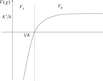
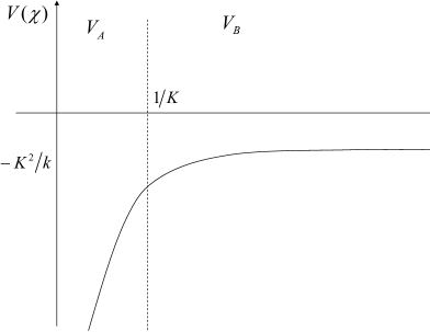
Figure 17: The potential $V(\chi)$ in Eq. (4.52) describing a Maxwell wave propagating in the $AdS_{5}$ geometry. Left: the space–like case ($\omega<k$). Right: the time–like case ($\omega>k$). In these figures, we denoted $K\equiv|k^{2}-\omega^{2}|^{1/2}$ (i.e. $K$ is the same as the variable $Q$ in the main text).

4.1 Space–like current

For a space–like current ($q^{2}>0$), one needs to take the upper sign in front of $Q^{2}$ in Eq. (4.52). The general solution is a linear combination of the modified Bessel functions $\mathrm{K}_{0}$ and $\mathrm{I}_{0}$ :

$$\psi(\chi)\,=\sqrt{\chi}\,\big{(}c_{1}\mathrm{K}_{0}(Q\chi)\,+\,c_{2}\mathrm{I}_{0}(Q\chi)\big{)}\,.$$ (4.53)

For large $x\equiv Q\chi\gg 1$,

$$\mathrm{K}_{0}(x)\,\approx\,\sqrt{\frac{\pi}{2x}}\,{\rm e}^{-x}\,,\qquad\mathrm{I}_{0}(x)\,\approx\,\frac{1}{\sqrt{2\pi x}}\,{\rm e}^{x}\,,$$ (4.54)

so the requirement that the solution remain regular as $\chi\to\infty$ selects $c_{2}=0$. The other coefficient $c_{1}$ is then fixed by the boundary condition at $\chi=0$, cf. Eq. (3.43), which becomes

$$\chi\,\frac{\partial}{\partial\chi}\,\frac{\psi}{\sqrt{\chi}}\Bigg{|}_{\chi\to 0}\,=\,2k\Big{(}kA_{0}^{(0)}+\omega A_{3}^{(0)}\Big{)}\,.$$ (4.55)

By also using the expansion $\mathrm{K}_{0}(x)\approx-\ln(x/2)-\gamma$ when $x\ll 1$, one easily finds $c_{1}=-2k\big{(}kA_{0}^{(0)}+\omega A_{3}^{(0)}\big{)}$. Via Eq. (3.46), the solution $\psi(\chi)$ determines the longitudinal piece of the classical action density, i.e., the pieces involving $A_{0}$ and $A_{3}$ in Eq. (3.45). A direct calculation yields

$$\mathcal{S}_{L}=\,-\frac{N^{2}_{c}}{64\pi^{2}}\,\big{(}qA_{0}^{(0)}+\omega A_{3}^{(0)}\big{)}^{2}\,\big{[}\ln{Q^{2}}+2\ln\chi+{\rm const.}\big{]}_{\chi=0}\,,$$ (4.56)

which however exhibits a logarithmic divergence as $\chi=0$. This might look disturbing at a first sight, but it has a natural resolution, that we shall now explain:

Field theories are well known to develop divergences in the limit where the ultraviolet cutoff (the upper cutoff on the momenta of the virtual corrections) is sent to infinity. These divergences can generally be eliminated via ultraviolet renormalization, i.e., by adding local ‘counterterms’ to the action, which amounts to (infinite) renormalizations of what we mean by the fields in the action, their masses, and their charges. In particular, the perturbative calculation of the polarization tensor within ${\mathcal{N}}=4$ SYM meets with logarithmic divergences of this type, which are then reabsorbed in the normalization of the ${\mathcal{R}}$–charge (or of the wavefunction of the ${\mathcal{R}}$–photon). But ultraviolet divergences and the need for renormalization are not restricted to perturbation theory, as shown by the example of lattice gauge theory. So, they are expected to appear also in the supergravity calculation, which must somehow encode the effects of all the quantum fluctuations of the dual gauge theory, including those with very high momenta. This discussion makes it plausible to interpret the logarithmic singularity in Eq. (4.56) as $\chi\to 0$ as the ‘dual counterpart’ of the respective ultraviolet divergence in the gauge theory. This is the content of the holographic renormalization [68, 69], which further instructs us to simply drop out this divergent term, possibly together with additional finite terms. Here we shall renormalize Eq. (4.56) by replacing

$$\ln{Q^{2}}+2\ln\chi+{\rm const.}\,\longrightarrow\,\ln\frac{Q^{2}}{\mu^{2}}\,,$$ (4.57)

which features the subtraction scale $\mu$. Via Eq. (3.44), this finally yields the function $\Pi(q^{2})$ displayed in Eq. (4.60) below (for $q^{2}>0$), and which is real, as expected: a space–like current cannot decay in the vacuum, by energy–momentum conservation. Interestingly, the holographic renormalization shows that there is a connection between the large momentum (more properly, large virtuality) limit in the original gauge theory and the limit $\chi\to 0$ (or $r\to\infty$) in the dual supergravity theory. This is a manifestation of the ultraviolet–infrared correspondence, that we shall later discuss in more detail.

4.2 Time–like current

The corresponding equation is obtained by takin the lower sign in front of $Q^{2}$ in Eq. (4.52). Then the general solution involves the oscillating Bessel functions $\mathrm{J}_{0}$ and $\mathrm{N}_{0}$ :

$$\psi(\chi)\,=\sqrt{\chi}\,\big{(}c_{1}\mathrm{J}_{0}(Q\chi)\,+\,c_{2}\mathrm{N}_{0}(Q\chi)\big{)}\,.$$ (4.58)

The condition of regularity as $\chi\to\infty$ is automatically satisfied by this general solution, so it brings no additional constraint. To fix the solution, we shall rather require $\psi(t,\chi)={\rm e}^{-i\omega t}\psi(\chi)$ to be an outgoing wave at large $\chi$, as explained in the previous section. This requires $c_{1}=-ic_{2}$ which together with the boundary condition (4.55) completely fixes the solution as

$$\psi(\chi)\,=\,-i\pi k\big{(}kA_{0}^{(0)}+\omega A_{3}^{(0)}\big{)}\sqrt{\chi}\,\mathrm{H}_{0}^{(1)}(Q\chi)\,,$$ (4.59)

where $\mathrm{H}_{0}^{(1)}=\mathrm{J}_{0}+i\mathrm{N}_{0}$ is a Hankel function encoding the desired outgoing–wave behavior at large $\chi$ : $\psi(t,\chi)\propto{\rm e}^{-i(\omega t-Q\chi)}$ when $\chi\gg 1/Q$. The remarkable feature of this solution is that it is complex, and thus it encodes dissipation. Specifically, the longitudinal piece of the action is obtained in the same form as in Eq. (4.56) except for an additional imaginary part. The would–be singular term at the boundary, which is real, is again removed as in Eq. (4.57), and the remaining, finite, part is finally used to compute the function $\Pi(q^{2})$.

One can combine together the results for both space–like and time–like currents in the following expression (recall that $Q^{2}=|q^{2}|$):

$$\Pi(q^{2})\,=\,\frac{N^{2}_{c}Q^{2}}{32\pi^{2}}\left(\ln\frac{Q^{2}}{\mu^{2}}-i\pi\Theta(-q^{2})\rm{sgn}(\omega)\right)\,,$$ (4.60)

where the imaginary part for the time–like case ($q^{2}<0$) is manifest. The sign of this imaginary part depends upon the sign of the energy, and is such as to correspond to retarded boundary conditions. Hence, as anticipated, Eqs. (4.51) and (4.60) present the exact result for the retarded, vacuum, polarization tensor of the ${\mathcal{R}}$–current in the ${\mathcal{N}}=4$ SYM theory at infinite ’t Hooft coupling. This has been obtained here via a classical calculation in the dual supergravity theory, but it also corresponds to an infinite resummation of (planar) Feynman diagrams of the original gauge theory. Can we say anything about the physics encoded in these diagrams ?

The first remarkable observation is that this all–order result in Eq. (4.60) is formally identical to the respective result at zero order in the Yang–Mills coupling $g$, i.e., the one–loop polarization tensor (see, e.g., the left figure in Fig. 10; recall that, in ${\mathcal{N}}=4$ SYM, this loop involves both adjoint quarks and adjoint scalars). This ‘coincidence’ is a consequence of supersymmetry which protects the conserved ${\mathcal{R}}$–current [70]; it means that all the higher loop corrections cancel each other, but it does not tell us much about the physical interpretation of the final result at strong–coupling. To gain more physical insight, we shall rely on the ultraviolet–infrared correspondence, that we shall first motivate, in the next subsection, on the basis of our previous results.

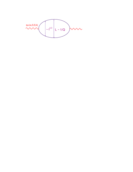
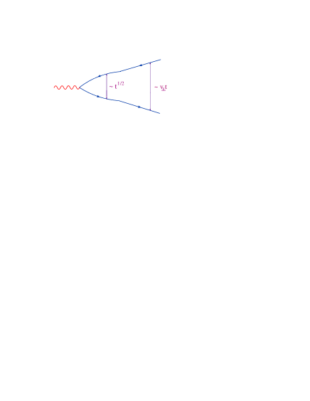
Figure 18: Space–time picture for the “one–loop” (one parton pair) fluctuation of a space–like current (left) and, respectively, time–like current (right).

4.3 The UV/IR correspondence

For a space–like current, we found that the Maxwell wave can penetrate into $AdS_{5}$ only up to a distance $\chi\sim 1/Q$ away from the boundary. This should be put in relation with the fact that, by energy–momentum conservation, a space–like current cannot decay in the vacuum, but it generally develops virtual, partonic, fluctuations (see Fig 18 left), with transverse size $L\sim 1/Q$ and lifetime $\Delta t_{\rm coh}$ which can be estimated from the uncertainty principle as

$$L\,\sim\,\frac{1}{Q}\,,\qquad\Delta t_{\rm coh}\,\sim\,\,\frac{1}{Q}\,\times\,\frac{k}{Q}\,\sim\,\frac{k}{Q^{2}}\,.$$ (4.61)

As suggested by the above writing, $\Delta t_{\rm coh}$ is obtained as the product between the lifetime $\sim 1/Q$ of the fluctuation in the frame in which the current has zero energy (its ‘rest frame’) and the Lorentz gamma factor $\gamma=k/Q$. We refer to this lifetime as a ‘coherence time’ since this is the interval during which the current acts as a color dipole, and hence it can interact via color gauge interactions. Quantum dynamics also provides us with a space–time picture for the fluctuation [71, 59]: if the photon dissociates at $t=0$ into a point–like pair of fermions, or scalars, then with increasing time the transverse size of this pair increases diffusively,

$$L\sim\sqrt{\frac{t}{k}}\,,$$ (4.62)

until it reaches its maximal size $L\sim 1/Q$ at a time $t\sim{k}/{Q^{2}}\sim\Delta t_{\rm coh}$.

Remarkably, it turns out that the very same space–time picture applies for the penetration of the Maxwell wave inside $AdS_{5}$ [31]. To see that, let us replace the plane–wave perturbation with a wave–packet which at $t=0$ is localized near the boundary. Then, as explained at the end of Sect. 3, the dynamics of the Maxwell wave $\psi(t,\chi)$ is governed by the time–dependent Schrödinger equation (3.50), which at early times (when the wave remains close to the boundary) reduces to

$$i\frac{\partial\psi}{\partial t}\,=\,\left(-\frac{1}{2k}\,\frac{\partial^{2}}{\partial\chi^{2}}\,-\,\frac{1}{8k\chi^{2}}\right)\psi\,.$$ (4.63)

This is valid for $\chi\lesssim 1/Q$, which corresponds to times $t\lesssim\Delta t_{\rm coh}$, as we shall shortly see. In this region, the $Q^{2}$–dependent piece in the potential in Eq. (4.52) is negligible, so this early–time dynamics is in fact the same for both space–like and time–like perturbations. Eq. (4.63) admits the following, exact solution

$$\psi(t,\chi)\,=\,-i\frac{\sqrt{\chi}}{t}\ {\rm e}^{i\frac{k\chi^{2}}{2t}}\,,$$ (4.64)

which is such that, as $t\to 0$, the actual field $a(t,\chi)\propto{\psi(\chi)}/{\sqrt{\chi}}$ (cf. Eq. (3.46)) is indeed localized near $\chi=0$, whereas for $t>0$ it penetrates into the bulk of $AdS_{5}$ through diffusion (i.e., by undergoing Brownian motion). This implies that the (typical) position of the center of the wave–packet after a time $t$ reads

$$\chi_{\rm diff}(t)\,\sim\,\sqrt{\frac{{t}}{k}}\,,$$ (4.65)

which becomes $\chi\sim 1/Q$ at time $t\sim{k}/{Q^{2}}$. For the space–like wave, this is the maximal penetration distance, as clear by inspection of Fig 19 left (and discussed in Sect. 4.1).

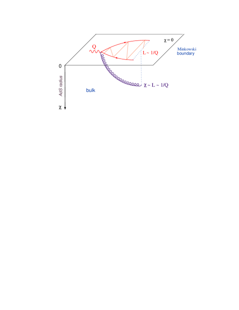
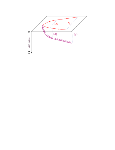
Figure 19: Graphical illustrations of the progression of the Maxwell wave in the radial dimension $\chi$ (the curly curve represents the trajectory of the wave–packet) and of the dual partonic fluctuation on the Minkowski boundary (which can be viewed as the ‘shadow’ of the Maxwell wave). Left: space–like case. Right: time–like case.

This precise analogy suggests an identification, or ‘duality’, between the penetration $\chi=R^{2}/r$ of the Maxwell wave inside $AdS_{5}$ and the transverse size $L$, or inverse virtuality $1/Q$, of the partonic fluctuation of the current in the gauge theory. This identification holds in the sense of a proportionality, so like the uncertainty principle:

Radial penetration $\chi=R^{2}/r$ in $AdS_{5}$   $\sim$   Transverse size $L\sim 1/Q$ on the boundary

This is a specific form of the ultraviolet–infrared correspondence of AdS/CFT [56, 51] within the context of the high–energy problem. This is often formulated as a correspondence between the 5th dimension and the ‘energy’ in the gauge theory. As such, this is correct at low energy, but in general the ‘energy’ should be replaced by the (boost–invariant) virtuality [57, 31]. As we shall see, this correspondence is very helpful in reconstructing the physical interpretation of the AdS/CFT results.

4.4 Parton branching at strong coupling

As a first application, consider the case of a time–like current. If at $t=0$ we start again with a wave–packet localized near $\chi=0$, then at early times $t\lesssim{\omega}/{Q^{2}}$ the dynamics will be the same as for a space–like current — the wave–packet slowly diffuses into the bulk up to a distance $\chi\sim 1/Q$ — but then the situation changes: instead of a potential barrier, the time–like wave meets with a flat potential, so it can freely propagates towards larger values of $\chi$ (cf. Figs. 17 and Fig 19 right). This is manifest from our previous solution (4.59): by using the asymptotic form of the Hankel function valid at $\chi Q\gg 1$ and restoring the exponential dependencies upon $t$ and $z$, one finds that the late–time solution behaves like

$${\rm e}^{-i\omega t+ikz}\,\frac{\psi}{\sqrt{\chi}}\,\propto\,\exp\left\{-i\omega t+ikz+iQ\chi\right\}\,.$$ (4.66)

This describes a wave–packet propagating in $AdS_{5}$ with constant radial velocity $v_{\chi}=Q/\omega$ :

$$\frac{\partial}{\partial\omega}\left(\omega t-\sqrt{\omega^{2}-k^{2}}\,\chi\right)\,=\,0\qquad\Longrightarrow\qquad\chi(t)\,=\,\frac{Q}{\omega}\,t\,\equiv\,v_{\chi}t\,.$$ (4.67)

At the same time, this wave–packet moves along the $z$ direction with constant velocity $v_{z}={k}/{\omega}$ (as obvious by taking a derivative in Eq. (4.66) w.r.t. $k$ at constant $Q$). $v_{z}$ is recognized as the longitudinal velocity of the incoming, time–like current. Notice that $v_{z}^{2}+v_{\chi}^{2}=1$, which is the velocity of light in $AdS_{5}$. We thus conclude that, for times $t>{\omega}/{Q^{2}}$, the wave–packet propagates in $AdS_{5}$ along a light–like geodesic.

Via the UV/IR correspondence $\chi\sim L$, these results predict the following behaviour on the gauge theory side (see Fig 19 right) : For times $t>{\omega}/{Q^{2}}$, the partonic system produced via the dissociation of the time–like current expands in transverse directions at a constant speed $v_{\perp}=v_{\chi}$ :

$$L(t)\,\sim\,v_{\perp}t\quad\mbox{with}\quad v_{\perp}\,=\,\frac{Q}{\omega}\,=\sqrt{1-v_{z}^{2}}\quad\mbox{where}\quad v_{z}\,=\,\frac{k}{\omega}\,.$$ (4.68)

This behaviour admits two different physical interpretations, but as we shall argue below only the second one is acceptable at strong coupling :

(i) The decay of the current into a pair of partons.
The time–like current decays into a pair of on–shell, massless partons (adjoint fermions or scalars) of ${\mathcal{N}}=4$ SYM theory, which then move together along the $z$ direction with a longitudinal velocity $v_{z}=k/\omega$ inherited from the current, while separating from each other in transverse directions at velocity $v_{\perp}=\sqrt{1-v_{z}^{2}}$.

This is, of course, the space–time picture of the one–loop approximation to $\Pi_{\mu\nu}$ and as such it must be consistent with the AdS/CFT calculation, since the result of the latter turns out to be formally the same as the respective one–loop result. But being ‘consistent’ it not necessarily the same as being correct. At strong coupling there is no reason why parton branching should stop at 2–parton level: it takes some time before the original pair of partons can get on–shell, and during this time they will further radiate, as the emission time is shorter than the time necessary to evacuate their virtuality. At weak coupling, such additional emissions are suppressed by powers of $g$, so they appear as higher–order corrections (cf. the discussion in Sect. 2). But at strong coupling, there is no such a suppression, and hence nothing can slow down the branching process, which is required by the uncertainty principle. Following the same idea, there is no reason why, at strong coupling, parton branching should favor special corners of the phase–space, like soft or collinear partons: phase–space enhancement is not needed when the coupling is strong. Such considerations suggest a space–time picture for parton evolution at strong coupling which is quite different from the corresponding one at weak coupling, and that we now present:

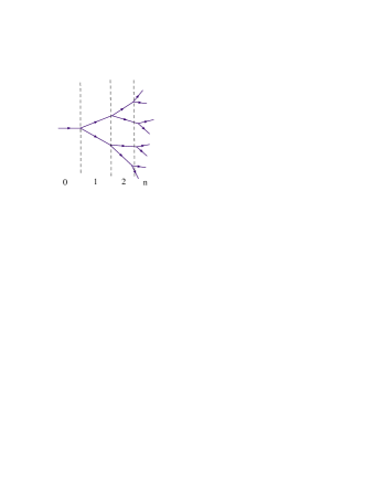
Figure 20: Qualitative picture of the parton cascade generated through ‘quasi–democratic’ branching at strong coupling. A line (‘branch’) with an arrow denotes any of the massless partons (quark, gluon, or scalar) of the ${\mathcal{N}}=4$ SYM Lagrangian, except possibly for the first parton, which initiates the cascade, which can also be a virtual $\mathcal{R}$–photon.

(ii) Quasi–democratic parton branching at strong coupling [31].
The virtuality of the current, or of any virtual parton which is time–like, is evacuated via successive parton branchings which are ‘quasi–democratic’: at each step in this branching process, the energy and virtuality are almost equally divided among the daughter partons. This picture, which is more acceptable at strong coupling, is indeed consistent with the previous AdS/CFT results, as we now show:

Let $n=0,1,2,\,...$ be the generation index, with $Q_{0}=Q$ and $\omega_{0}=\omega$ (see Fig. 20). Then we can write

$$\omega_{n}\,\sim\,\frac{\omega_{n-1}}{2}\,\sim\,\frac{\omega}{2^{n}}\,,\qquad Q_{n}\,\sim\,\frac{Q_{n-1}}{2}\,\sim\,\frac{Q}{2^{n}}\,,\qquad\Delta t_{n}\,\sim\,\frac{\omega_{n}}{Q_{n}^{2}}\,,$$ (4.69)

where the lifetime $\Delta t_{n}$ of the $n$th parton generation has been estimated via the uncertainty principle. This implies

$$\frac{Q_{n}-Q_{n-1}}{\Delta t_{n}}\,\sim\,-\,\frac{Q}{\omega}\,Q_{n}^{2}\quad\Longrightarrow\quad\frac{{\rm d}Q(t)}{{\rm d}t}\,\simeq\,\,-\,\frac{Q^{2}(t)}{\gamma}\,,$$ (4.70)

where $\gamma\equiv\omega/Q=1/\sqrt{1-v_{z}^{2}}$ is the Lorentz factor for both the incoming, time–like, current and any of the virtual partons produced via its decay: indeed, the ratio $\omega_{n}/Q_{n}\approx\omega/Q$ is approximately constant during the branching process, hence $\gamma_{n}\approx\gamma$. This means that each parton generation progresses along the longitudinal direction at the same speed $v_{z}$ as the original current would do. But at the same time the virtuality decreases from one generation to another, hence the partonic system expands in transverse directions. Specifically, Eq. (4.70) together with the uncertainty principle $L(t)\sim 1/Q(t)$ implies that the transverse size of the partonic system increases like $L(t)\sim\sqrt{1-v_{z}^{2}}\,t$, in qualitative agreement with the AdS/CFT result in Eq. (4.68).

By integrating Eq. (4.70), one can deduce the virtuality $Q(t)$ and the energy $\omega(t)=\gamma Q(t)$ that a typical parton in the cascade will have after a time $t\geq\Delta t_{0}\sim\omega/Q^{2}$. One thus finds

$$Q(t)\,\simeq\,\frac{\gamma}{t}\,,\qquad\omega(t)\,\simeq\,\frac{\gamma^{2}}{t}\,.$$ (4.71)

(For $t=\omega/Q^{2}$, these equations yield $Q(t)=Q$ and $\omega(t)=\omega$, as they should.) Of course, the total energy of the partonic system is conserved and equal to $\omega$ (the energy of the incoming photon), but with increasing time this energy gets spread among more and more partons. One can indeed check that the number of partons within the cascade increases like $N_{\rm part}(t)\simeq t/\Delta t_{0}$.

For how long will this branching process last ? Within the conformal ${\mathcal{N}}=4$ SYM theory, the partons will keep branching for ever, thus producing more and more partons, with lower and lower energies. But if one introduced a infrared cutoff $\Lambda$ in the theory, as a crude model to mimic confinement and ensure the existence of hadron–like states, then the branching will continue until the parton virtualities degrade down to values of order $\Lambda$; then hadrons will form and the particle distribution will get frozen. The total duration of the branching process is essentially the same as the lifetime $\Delta t_{N}$ of the last generation, the one with $Q_{N}\sim\Lambda$. (Indeed the parton lifetime increases down the cascade: $\Delta t_{n}\simeq 2\Delta t_{n-1}\simeq 2^{n}\Delta t_{0}$.) This yields $\Delta t_{N}\sim 2^{N}(\omega/Q^{2})\sim\gamma/\Lambda$, where we have used $2^{N}=Q/\Lambda$ and $\omega/Q=\gamma$. The final partons produced in this process are relatively numerous ($N_{\rm part}\sim 2^{N}=Q/\Lambda\gg 1$) and have small transverse momenta $k_{\perp}\sim Q_{N}\sim\Lambda$, so they will be isotropically distributed in transverse space, within a disk with area $\sim 1/\Lambda^{2}$ around the longitudinal axis.

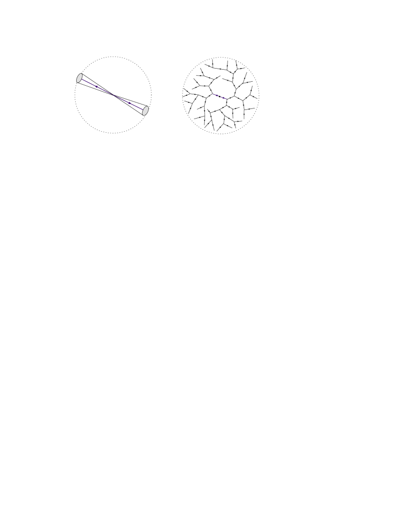
Figure 21: Final state produced in $e^{+}e^{-}$ annihilation. Left: weak coupling. Right: strong coupling.

This picture of ‘quasi–democratic branching’ — that one should think off as a kind of mean field approximation to the actual dynamics in the gauge theory at strong coupling — has intriguing consequences for processes like $e^{+}e^{-}$ annihilation at high energy ($\sqrt{s}\gg\Lambda$). Consider the respective final state as seen in the center of mass frame. Unlike what happens in QCD at weak coupling, where this state involves only a few, well collimated, jets (cf. Sect. 2 and Fig. 21 left), at strong coupling there will be no jets at all ! Rather, the final hadrons will be relatively soft — they all carry energies and momenta of order $\Lambda$ —, numerous and isotropically distributed in space, as illustrated in the r.h.s. of Fig. 21. (See also Refs. [72, 73, 74, 75] for different arguments leading to similar conclusions.) Such a structure for the final state is clearly inconsistent with what is actually seen in the high–energy experiments, and this should not come as a surprise: as argued in Sect. 2 (see, e.g., Eq. (2.10)), the decay of a highly–energetic time–like current in QCD is rather controlled by weak coupling, because of asymptotic freedom. One may nevertheless hope that strong–coupling techniques like AdS/CFT could be more useful when the current propagates through a finite–temperature plasma, where the relevant coupling is believed to be stronger. This is the topics that we shall discuss in the next section.

5 ${\mathcal{R}}$–current in the ${\mathcal{N}}=4$ SYM plasma at strong coupling

We are now prepared to address the problem which is our main physical interest, namely the propagation of the ${\mathcal{R}}$–current through the strongly coupled ${\mathcal{N}}=4$ SYM plasma. As we shall see, the corresponding AdS/CFT results are again suggestive of a ‘quasi–democratic branching’ picture, which is now generalized to accommodate the effects of the plasma.

We focus on a current with large virtuality, $Q\gg T$ (‘hard probe’), which therefore explores the structure of the plasma on distances short as compared to the thermal wavelength $1/T$. We shall perform our calculations in the plasma rest frame, but then interpret the results in the plasma infinite momentum frame, in order to unveil the partonic structure of the plasma. It is moreover interesting to choose this current to have a relatively high longitudinal momentum in the plasma rest frame, such that $k\gg Q\gg T$ (which in turn implies a high energy: $\omega\sim k$; recall that $Q^{2}\equiv|k^{2}-\omega^{2}|$). Indeed, below Eq. (4.61) we have argued that the interactions of the current with an external target extend over a time $\Delta t_{\rm coh}\sim k/Q^{2}$, i.e., the lifetime of its partonic fluctuation. For the current to explore medium properties in the plasma, we would like this time to be much larger than $1/T$ — so that the current explores a relatively large longitudinal slice $\Delta z\sim\Delta t_{\rm coh}\gg 1/T$. This implies $k\gg Q^{2}/T$ (and hence $k\simeq\omega\gg Q$), which is tantamount to the condition that the associated Bjorken–$x$ variable be very small: $x\ll 1$. (This variable will be introduced in Eq. (5.74) below.) In fact, as we shall later discover, for a space–like current to significantly interact with the plasma we need an even higher energy $\omega\gtrsim Q^{3}/T^{2}$ [30].

For an ordinary plasma at weak coupling, this physical set–up would probe the parton evolution of the individual thermal quasiparticles, so the plasma structure functions would be simply the sum of the structure functions for those quasiparticles weighted by the respective densities in thermal equilibrium. For instance, the gluon distribution per unit volume in the weakly–coupled quark–gluon plasma is given by

$$xg(x,Q^{2})\,\approx\,n_{q}(T)xg_{q}(x,Q^{2})\,+\,n_{g}(T)xg_{g}(x,Q^{2})\,,$$ (5.72)

where $n_{q}(T)\sim N_{c}T^{3}$ and $n_{g}(T)\sim N_{c}^{2}T^{3}$ are the thermal densities for (anti)quarks and gluons, and $xg_{q}(x,Q^{2})$ and $xg_{g}(x,Q^{2})$ are gluon distribution functions generated by the evolution of a single quark, or gluon, respectively. However, at strong coupling, the quasiparticle structure of the plasma is not known (if any !) and, moreover, we expect the evolution of the plasma as whole to be different from that of its individual constituents taken separately (once again, assuming that such individual constituents exist in the first place, which may not be true !). It then becomes interesting and meaningful to compute directly the plasma structure functions. This calculation refers to a space–like current, but a time–like current is interesting too, since this decays into jets, which then interact with the plasma. In what follows we shall consider both space–like and time–like currents, but we shall skip most technical details and focus on the results and their physical interpretation.

5.1 Space–like current: DIS off the strongly coupled plasma

Let us start with some kinematics. The polarization tensor in the plasma, as defined in Eq. (3.34), involves two independent scalar functions, $\Pi_{1}$ and $\Pi_{2}$, and admits the following decomposition in a generic frame:

$$\Pi_{\mu\nu}(q,T)=\left(\eta_{\mu\nu}-\frac{q_{\mu}q_{\nu}}{Q^{2}}\right)\Pi_{1}(x,Q^{2})+\left(n_{\mu}-q_{\mu}\frac{n\cdot q}{Q^{2}}\right)\left(n_{\nu}-q_{\nu}\frac{n\cdot q}{Q^{2}}\right)\Pi_{2}(x,Q^{2})\,.$$ (5.73)

Here $n^{\mu}$ is the four–velocity of the plasma, with $n^{\mu}=(1,0,0,0)$ corresponding to the plasma at rest. Also, the Bjorken–$x$ variable for the current–plasma scattering is defined as

$${x}\,\equiv\,\frac{Q^{2}}{-2(q\cdot n)T}\,=\,\frac{Q^{2}}{2\omega T}\,,$$ (5.74)

with the second expression valid in the plasma rest frame, where $q^{\mu}=(\omega,0,0,k)$. The plasma structure functions are obtained as

$$F_{1}(x,Q^{2})\,=\,\frac{1}{2\pi}\,{\rm Im}\,\Pi_{1},\qquad F_{2}(x,Q^{2})\,=\,\frac{-(n\cdot q)}{2\pi T}\,{\rm Im}\,\Pi_{2}\,.$$ (5.75)

This tensorial structure is similar to that introduced in Sect. 2 for DIS off a hadron, and the above formulae correspond indeed to Eqs. (2.16) and (2.17) up to the replacement $P^{\mu}\to n^{\mu}$. But unlike the hadronic polarization tensor, or structure functions, which are dimensionless, their plasma counterparts in Eqs. (5.73)-(5.75) have dimensions of momentum squared. This difference is related to their physical interpretation that we shall later discuss.

In order to compute $\Pi_{1}$ and $\Pi_{2}$ from classical supergravity, we need to solve the equations for both the transverse and longitudinal Maxwell waves, that is, Eqs. (3.39) and (3.42), respectively. There is an important simplification which simplifies this analysis: the most important dynamics takes plays relatively far away from the BH horizon, at $\chi\ll\chi_{0}$, where $f(\chi)\approx 1$ (cf. Eq. (3.30)). Of course, the absorbtion of the wave by the BH takes place around the horizon, but the effects of the interactions with the BH makes themselves felt already well above $\chi_{0}$, because of the long range nature of the gravitational interactions (see below); in turn, these long–range interactions uniquely determine the classical solution near the Minkowsky boundary ($\chi\to 0$), which is all that we need in order to compute the polarisation tensor (cf. Eq. (3.45)). Because of that, we can replace $f\to 1$ (i.e., ignore the effects of the BH) everywhere except in the terms where the difference $1-f=(\chi/\chi_{0})^{4}$ is amplified by the large longitudinal momentum of the current. To be more specific, let us consider the longitudinal sector and use the form (3.47) of the respective EOM. The third term in this equation involves

$$\omega^{2}-k^{2}f(\chi)\,=\,\omega^{2}-k^{2}+k^{2}\,\frac{\chi^{4}}{\chi_{0}^{4}}\,=\,\mp Q^{2}+\big{(}\pi^{2}kT^{2}\chi^{2})^{2}\,,$$ (5.76)

(as usual, the upper/lower sign in front of $Q^{2}$ corresponds to a space–like/time–like current, respectively), where the last term $\propto k^{2}T^{4}$ becomes comparable with $Q^{2}$ for any $\chi$ greater than a ‘critical’ value $\chi_{\rm cr}=\chi_{0}\sqrt{Q/k}$. Note that, in the high–energy of interest here ($k\gg Q$), this value $\chi_{\rm cr}$ is much smaller than $\chi_{0}$ and in fact it can be arbitrarily small. Hence this piece of the gravitational interactions — which describes the Newton potential created by the BH (or one graviton exchange) — can be important even far away from the horizon, including in the vicinity of the boundary. This is the piece of the interaction that we must keep. But all the other factors of $f$ appearing in Eq. (3.47) can be safely replaced by 1 so long as we restrict ourselves to $\chi\ll\chi_{0}$, which we shall do indeed in what follows. Then the respective equation of motion (including time–dependence) takes indeed the form of a Schrödinger equation, as anticipated at the end of Sect. 3:

$$i\frac{\partial\psi}{\partial t}\,=\,-\frac{1}{2k}\,\frac{\partial^{2}\psi}{\partial\chi^{2}}\,+\,V(\chi)\psi\,,\qquad V(\chi)\,=\,-\,\frac{1}{8k\chi^{2}}\,\pm\,\frac{Q^{2}}{2k}\,-\,\frac{k}{2}\,\frac{\chi^{4}}{\chi_{0}^{4}}\,.$$ (5.77)

The respective roles of the three pieces in the potential should be clear by now: (a) the first piece ($V_{A}$), which is independent of both the virtuality and the temperature, describes the diffusive penetration of the wave at early times (or, in the dual gauge theory, the diffusive growth of the partonic fluctuation of the current in transverse directions); (b) the second one ($V_{B}$), which is flat and proportional to $Q^{2}$, is the potential barrier which prevents a space–like current to decay into the vacuum, and (c) the third piece ($V_{C}$) is the one–graviton exchange interaction between the current and the BH. We shall latter attempt to provide a physical interpretation for this last piece on the gauge theory side. The balance between these three pieces depends upon the energy $\omega\simeq k$ and the virtuality $Q^{2}$ of the current, and upon the temperature. There are two important physical regimes, a low energy one and a high energy one, which for the space–like current are illustrated in Fig. 22. The transition between these two regimes occurs at an energy $\omega\sim Q^{3}/T^{2}$, as we now explain:

  

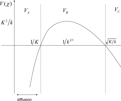
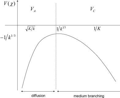
Figure 22: The potential $V(\chi)$ in Eq. (5.77) in the space–like case (upper sign in front of $Q^{2}$). Left: low–energy case ($\omega\ll Q^{3}/T^{2}$). Right: high–energy case ($\omega\gtrsim Q^{3}/T^{2}$). Note that, in the high–energy case the potential looks qualitatively similar for a time–like current as well. (In these figures, $Q$ is denoted as $K$, and all variables have been made dimensionless by multiplying with appropriate powers of $T$.)

(i) Low energy: $\omega\ll\omega_{s}\equiv Q^{3}/T^{2}$ (see Fig. 22 left)
So long as the energy is relatively low (with $\omega\gg Q^{2}/T\gg Q$ though), the potential shows a barrier corresponding to energy–momentum conservation, so like in the vacuum (compare to Fig. 17 left). However, and unlike in the vacuum, this barrier has now only a finite width — it extends over the interval $1/Q\lesssim\chi\lesssim\chi_{\rm cr}$, with $\chi_{\rm cr}=\chi_{0}\sqrt{Q/k}$ —, and for larger $\chi\gg\chi_{\rm cr}$ we have $V\simeq V_{C}$ which describes attraction by the BH. Hence, there is a small, but non–vanishing, probability for the wave to penetrate through the barrier via tunnel effect, and once that this happens the wave will fall into the BH. This tunnel effect will provide an exponentially small contribution to the imaginary part of the polarization tensor, and hence to the structure functions, which can be estimated in the WKB approximation as (parametrically) [30]

$$F_{2}\,\sim\,xF_{1}\,\sim\,x{N^{2}_{c}Q^{2}}D\,,\qquad D\,\sim\,\exp\Big{\{}-c(\omega_{s}/\omega)^{1/2}\Big{\}}\,=\,\exp\left\{-c\,\frac{Q}{\sqrt{\gamma}\,T}\right\}\,,$$ (5.78)

where $c$ is some undetermined numerical coefficient and we have used $\gamma=\omega/Q$. Interestingly, the exponential attenuation factor $D$ which is generated through tunneling looks formally like a Boltzmann thermal factor $\exp(-Q/T_{\rm eff})$ with an effective temperature $T_{\rm eff}=\sqrt{\gamma}\,T$. One can understand $T_{\rm eff}$ as the temperature of the plasma in a boosted frame in which the current has zero longitudinal momentum (and hence the plasma has a large global velocity $\omega/k\simeq 1$): indeed, the energy density of the plasma, which in the plasma rest frame scales like $\mathcal{E}\equiv T_{00}\sim N_{c}^{2}T^{4}$, becomes $\mathcal{E}^{\prime}=\gamma^{2}\mathcal{E}$ in the boosted frame; this is the same energy density as for a plasma at rest but with an effective temperature $\sqrt{\gamma}\,T$.

We conclude that the low–energy space–like current can decay inside the plasma, albeit very slowly. We shall later interpret this decay as pair production induced by a uniform background force — that is, a kind of Schwinger mechanism.

(ii) High energy: $\omega\gg\omega_{s}\equiv Q^{3}/T^{2}$ (see Fig. 22 right)
With increasing energy at fixed $T$ and $Q^{2}$, $\chi_{\rm cr}$ becomes smaller and smaller, so the barrier becomes narrower and it eventually disappears: this happens when $\chi_{\rm cr}\sim 1/Q$, or $\omega\sim\omega_{s}$. For even higher energies we are in the situation illustrated in Fig. 22 right, where the wave can move all the way up to the horizon, where it is ultimately absorbed with probability one. From the point of view of DIS, this situation corresponds to the unitarity, or ‘black disk’, limit (the strongest possible scattering).

In this high energy regime, the virtuality–dependent term $V_{B}$ in the potential is comparatively small at any $\chi$ and thus can be neglected. We conclude that, for such a high energy, the dynamics is in fact the same for both space–like and time–like currents; and, of course, it would be the same also for a light–like current ($Q^{2}=0$) with high energy $\omega\gg T$. Then $V(\chi)\simeq V_{A}+V_{C}$ has a maximum at $\chi=\chi_{s}$ with

$$\chi_{s}\,\sim\,\frac{1}{T}\,\left(\frac{T}{\omega}\right)^{1/3}=\,\frac{1}{Q_{s}}\,,$$ (5.79)

which is far away from the horizon: $\chi_{s}\ll 1/T\sim\chi_{0}$. Above, we have introduced the plasma saturation momentum

$$Q_{s}(\omega,T)\,\sim\,({\omega}T^{2})^{1/3}\,,\qquad\mbox{or}\qquad Q_{s}(x,T)\,\sim\,\frac{T}{x}\,,$$ (5.80)

which is the virtuality which separates between the (almost) no–scattering regime at $Q\gg Q_{s}$ and the strong scattering regime at $Q\lesssim Q_{s}$. In other terms, the strong–scattering condition $\omega\sim Q^{3}/T^{2}$ can be solved either for $\omega$, thus yielding $\omega\sim\omega_{s}$, or for $Q$, which gives $Q\sim Q_{s}$. We shall later argue that, also in this context at strong coupling, the scale $Q_{s}$ is associated with the phenomenon of parton saturation, so like in QCD at weak coupling (cf. Sect. 2).

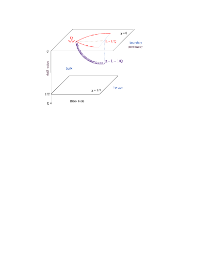
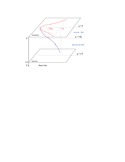
Figure 23: Space–like current in the plasma: the trajectory of the wave packet in $AdS_{5}$ and its ‘shadow’ on the boundary. Left: the (relatively) low energy case — the Maxwell wave gets stuck near the boundary up to tunnel effect. Right: the high energy case — the wave has an accelerated fall into the BH.

The high–energy dynamics thus proceeds as follows (for either space–like or time–like current; see also Fig. 23 right): Starting at $t=0$ with a wave–packet localized near the boundary ($\chi=0$), this will slowly diffuse inside the bulk, so like in the vacuum (cf. Eq. (4.65)), up to a distance $\chi\sim\chi_{s}$ where it starts feeling the BH. This takes a time $t_{s}$ determined as

$$\chi(t)\,\sim\,\sqrt{\frac{{t}}{\omega}}\quad{\rm\&}\quad\chi(t_{s})\,\sim\,\chi_{s}\quad\Longrightarrow\quad t_{s}\,\sim\,\frac{\omega}{Q_{s}^{2}}.$$ (5.81)

Then, the wave falls towards the BH following an accelerated trajectory which, interestingly, brings the wave–packet in the vicinity of the horizon ($\chi(t)\sim\chi_{0}$) at a time $t_{f}$ which is parametrically of the same order as $t_{s}$. This can be understood as follows: in the semi–classical, WKB, approximation, the center of the wave–packet moves in the same way as a classical particle with mass $k$ in the potential $V\simeq V_{c}$ and with zero total (kinetic plus potential) energy. The last condition reads

$$T\,+\,V_{c}\,=\,\frac{k\dot{\chi}^{2}}{2}\,-\,\frac{k}{2}\,\frac{\chi^{4}}{\chi_{0}^{4}}\,=\,0\quad\Longrightarrow\quad\frac{{\rm d}\chi}{{\rm d}t}\,=\,\frac{\chi^{2}}{\chi_{0}^{2}}\,,$$ (5.82)

which is easily integrated starting at time $t=t_{s}$ to yield

$$\chi(t)\,=\,\frac{\chi_{s}}{1-\frac{\chi_{s}}{\chi_{0}^{2}}(t-t_{s})}\,.$$ (5.83)

This $\chi(t)$ approaches $\chi_{0}\gg\chi_{s}$ when the denominator is almost vanishing, which implies

$$t_{f}-t_{s}\,\simeq\,\frac{\chi_{0}^{2}}{\chi_{s}}\,\sim\,\frac{Q_{s}}{T^{2}}\,\sim\,\frac{\omega}{Q_{s}^{2}}\,\sim\,t_{s}\,.$$ (5.84)

Thus, as anticipated, the total fall time (defined as the time after which the wave packet arrives in the vicinity of the horizon) reads, parametrically,

$$t_{s}\,\sim\,\frac{\omega}{Q_{s}^{2}}\,\sim\,\frac{1}{T}\,\left(\frac{\omega}{T}\right)^{1/3}\,.$$ (5.85)

From the perspective of the dual gauge theory, this time $t_{s}$ is the lifetime of the high energy current before being absorbed by the plasma. Since, moreover, the current propagates essentially at the speed of light (at least, before it starts to feel the plasma), $t_{s}$ also gives also the penetration length for the high energy current, i.e., longitudinal distance $\Delta z$ traveled by the current before disappearing in the plasma. As shown by the above estimate, $\Delta z$ scales like ${\omega}^{1/3}$, which is also the law found for a falling open string (the dual of a ‘massless gluon’) in Refs. [48, 50]. This similarity points towards the universality of the mechanism for energy loss in the strongly coupled plasma, that we shall describe in Sect. 5.3.

To compute the plasma structure functions in this high–energy regime, it is enough to consider the time–independent version of the ‘Schrödinger equation’ (5.77) with the simplified potential $V=V_{A}+V_{C}$ (together with a similar equation for the transverse waves [30]). The details of the geometry near the BH horizon are again irrelevant, since the outgoing–wave boundary condition can be enforced already at relatively small distances $\chi\ll\chi_{0}$, namely at any $\chi\gg\chi_{s}$. (Recall that $\chi_{s}=1/Q_{s}\ll\chi_{0}$.) Then the classical solutions are fixed at all smaller values of $\chi$ and, in particular, near the Minkowski boundary. One thus obtains the following parametric estimates for $F_{1,2}$ [30]

$$F_{2}\,\sim\,xF_{1}\,\sim\,x{N^{2}_{c}Q^{2}}\left(\frac{T}{xQ}\right)^{2/3}\quad\mbox{for}\quad Q\,\lesssim\,Q_{s}(x,T)\,=\,\frac{T}{x}\,.$$ (5.86)

A physical interpretation for this result will be presented in Sect. 5.4.

Note finally that the lifetime (5.85) of the high–energy current is formally the same as the coherence time for a current with virtuality equal to $Q_{s}$ (and not to $Q$ !). Since $Q_{s}\gg Q$ in this regime, it is clear that $t_{s}\ll\Delta t_{\rm coh}(Q)$: that is, the current disappears in the plasma before having the time to develop a normal partonic fluctuation with size $L\sim 1/Q$, as it would do in the vacuum. This has interesting consequences for the survival of a ‘meson’ state in the plasma:

A high–energy space–like current is the simplest device to create a ‘meson’, i.e., a partonic excitation which is overall color neutral but has a non–zero color dipole moment. This is, of course, a virtual excitation and not a truly bound state, but its lifetime $\Delta t_{\rm coh}\sim\omega/Q^{2}$ can be made arbitrarily large by increasing the energy $\omega$ of the current (for a given transverse size $L\sim 1/Q$). At least, this is the situation in the vacuum. But what about the strongly–coupled plasma ? There, a similar situation holds too, but only so long as the energy of the current is not too high: namely, when $\omega\ll\omega_{s}\sim Q^{3}/T^{2}$, the ‘mesonic’ fluctuation lives nearly as long as in the vacuum, since its interactions with the plasma are exponentially suppressed. But for higher energies $\omega\gtrsim Q^{3}/T^{2}$, the current is absorbed already before having the time to create a meson. This puts an upper limit on the ‘rapidity’ $\gamma\equiv\omega/Q$ of the meson (with a given size $L$) that can be created by a high energy process occurring within the plasma (‘limiting velocity’) :

$$\gamma_{\rm max}\,\sim\,\frac{\omega_{s}}{Q}\,\sim\,\frac{Q^{2}}{T^{2}}\,\sim\,\frac{1}{(LT)^{2}}\,,$$ (5.87)

or, alternatively, an upper limit on its transverse size for a given value of $\gamma$ (‘screening length’) :

$$L_{\rm max}\,\sim\,\frac{1}{Q_{s}}\,\sim\,\frac{Q^{2}_{s}}{\omega T^{2}}\,\sim\,\frac{1}{\gamma L_{\rm max}T^{2}}\quad\Longrightarrow\quad L_{\rm max}\,\sim\,\frac{1}{\sqrt{\gamma}\,T}\,.$$ (5.88)

(Notice the emergence of the effective temperature $T_{\rm eff}=\sqrt{\gamma}\,T$.) Similar limits have been found in a different approach [41, 42, 43, 44, 45], in which the ‘meson’ is viewed as a quark–antiquark pair (with heavy quarks), whose string dual is an open string with endpoints attached to a D7–brane embedded in the $AdS_{5}$–BH geometry. This similarity between seemingly different physical problems and approaches — $\mathcal{R}$–current vs. open string, heavy quarks vs. massless quanta of ${\mathcal{N}}=4$ SYM — points, once again, towards an universal mechanism for energy loss at strong coupling. We shall present our conjecture [31] for this mechanism in Sect. 5.3, after the discussion of the time–like current in the plasma. Before concluding, let us also mention a difference between our results and those based on the open string picture for the meson: in the low–energy/small–size regime where the meson can form in the plasma, our approach predicts that the meson can decay, albeit very slowly, via tunneling (the corresponding width is exponentially small, cf. Eq. (5.78)), whereas in the approach of Refs. [41, 42, 43] one finds that the width is strictly zero (the lifetime of the meson is infinite). Very recently, finite–width effects have been added to the string picture in Ref. [47], as string worldsheet instantons; it would be interesting to clarify the relation between these new results and those in Eq. (5.78).

5.2 Time–like current: $e^{+}e^{-}$ annihilation in a strongly coupled plasma

The evolution of a time–like current in the plasma should in principle teach us about the behaviour of nearly on–shell partonic jets which are produced by a high–energy process, so like $e^{+}e^{-}$ annihilation, taking place within the plasma. From the previous discussion, we know already that, at strong coupling, the situation is in fact more subtle. First, even in the vacuum, the partons created by the decay of the time–like current are far from being on–shell, at least in the early stages of the branching process. Second, if the energy $\omega$ is high enough, such that $\omega/Q\gtrsim(Q/T)^{2}$, then the current disappears so fast into the plasma that it cannot even create the kind of partonic fluctuation that it would develop into the vacuum. In other terms, the virtual partons that the current fluctuates into have even larger virtualities, of order $Q_{s}\gg Q$.

This last case, that of a highly–energetic current, has been already covered in the previous subsection: indeed, the respective dynamics is insensitive to the virtuality $Q^{2}$, and hence it is the same for time–like, space–like, or even light–like, currents. Before we propose a physical interpretation for this dynamics, let us first consider the only remaining case, that of a time–like current at relatively low energy: $\omega\ll\omega_{s}\equiv Q^{3}/T^{2}$ (with $\omega\gg Q^{2}/T\gg Q$ though).

      

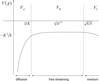
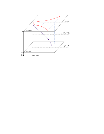
Figure 24: Left: the potential $V(\chi)$ in Eq. (5.77) in the time–like case (lower sign in front of $Q^{2}$). Right: the trajectory of the Maxwell wave–packet in $AdS_{5}$ and its ‘shadow’ on the Minkowski boundary. In the left figure one uses dimensionless variables together with the notation $K\equiv Q$; e.g. $\chi\sim\sqrt{K/k}$ in the left figure is the same as $\chi\sim 1/(\gamma^{1/2}T)$ in the right figure.

The respective potential, as obtained by taking the lower sign in front of $Q^{2}$ in Eq. (5.77), is displayed in Fig. 24 left, which should be compared to the respective potential in the vacuum, cf. Fig. 17 right, and also to the space–like potential in Fig. 22 left. Similarly to the space–like case, there is a critical radial distance $\chi_{\rm cr}=\chi_{0}\sqrt{Q/\omega}$ below which the Maxwell wave does not feel the plasma. However, unlike in tat case, now there is no potential barrier anymore, so even for a relatively low energy the time–like wave can propagate up to this critical distance and then start its fall into the BH. Note that one can also write $\chi_{\rm cr}=\chi_{0}/\sqrt{\gamma}$ since $\gamma=\omega/Q$.

For $\chi\ll\chi_{\rm cr}$, meaning at early times, the dynamics is the same as for a time–like current in the vacuum (cf. Sect. 4) : (i) The Maxwell wave–packet first diffuses inside the bulk up to a distance $\chi_{1}\sim 1/Q$; this takes a time $t_{1}\sim\omega/{Q^{2}}$ (the coherence time for the virtual photon). (ii) Then, the potential becomes flat, so the wave–packet propagates at constant radial speed $v_{\chi}=Q/\omega$ up to a distance $\chi_{\rm cr}\gg 1/Q$; this takes an additional time

$$t_{c}-t_{1}\,\simeq\,\frac{\chi_{\rm cr}}{v_{\chi}}\,\sim\,\frac{1}{T}\,\sqrt{\frac{\omega}{Q}}\ \gg\ t_{1}\,\sim\,\frac{\omega}{Q^{2}}\,,$$ (5.89)

which is much larger than $t_{1}$; therefore, $t_{c}\simeq t_{c}-t_{1}\sim\sqrt{\gamma}/T$. (iii) For $\chi\gtrsim\chi_{\rm cr}$, $V\simeq V_{c}$ and the wave–packet falls towards the horizon according to the same law as for the high–energy regime discussed in the previous subsection, cf. Eqs. (5.82)–(5.83). The only difference is that, now, this fall begins at a different time ($t_{c}$ instead of $t_{s}$) and at a different radial location ($\chi_{\rm cr}$ instead of $\chi_{s}$). Hence the trajectory of the center of the wave–packet now reads (compare to Eq. (5.83))

$$\chi(t)\,=\,\frac{\chi_{\rm cr}}{1-\frac{\chi_{\rm cr}}{\chi_{0}^{2}}(t-t_{c})}\,,$$ (5.90)

so that the traveling time $t_{f}-t_{c}$ down to the vicinity of the horizon is now of order $t_{c}$ :

$$t_{f}-t_{c}\,\simeq\,\frac{\chi_{0}^{2}}{\chi_{\rm cr}}\,\sim\,\frac{1}{T}\,\sqrt{\frac{\omega}{Q}}\,\sim\,t_{c}\,.$$ (5.91)

Eq. (5.82) shows that the radial velocity $v_{\chi}\equiv{{\rm d}\chi}/{{\rm d}t}$ increases with time, due to the attraction exerted by the BH, and becomes of $\mathcal{O}{(1)}$ when $\chi\sim\chi_{0}$. One can similarly show that, at times $t>t_{c}$, the motion of the wave–packet along the $z$ axis is decelerated according to

$$v_{z}(t)\,\equiv\,\frac{{\rm d}z}{{\rm d}t}\,\simeq\,1\,-\,\frac{\chi^{4}}{\chi_{0}^{4}}\,,$$ (5.92)

and thus it approaches to zero when the wave–packet approaches the horizon. Note that, within the present approximations (which are valid so long as $\chi\ll\chi_{0}$), the total velocity remains luminal, $v_{z}^{2}+v_{\chi}^{2}=1$, even during the phase of fall towards the BH. This is suggestive of a partonic interpretation in terms of massless partons which are eventually stopped into the plasma. We shall elaborate on this interpretation in Sect. 5.3.

These results also show that the wave–packet falls into the BH along a light–like geodesic. More precisely, the trajectory of the light–like geodesic in the $AdS_{5}$–BH geometry reads (see, e.g., [48, 50]) :

$$\frac{{\rm d}z}{{\rm d}t}\,=\,vf(\chi(t))\,,\qquad\frac{{\rm d}\chi}{{\rm d}t}\,=\,f\sqrt{1-v^{2}f}\,,$$ (5.93)

with $f(\chi)$ as defined in Eq. (3.30) and $v\leq 1$ the longitudinal velocity near the boundary. We have indeed: $({\rm d}z)^{2}+(1/f)({\rm d}\chi)^{2}=f({\rm d}t)^{2}$, as it should for a light–like geodesic in this particular geometry. When $v\simeq 1$ and $\chi\ll\chi_{0}$, the equations (5.93) are fully consistent with our previous results for the propagation of the wave–packet at times $t>t_{1}$ (i.e., after the early diffusion). For instance the second equation (5.93) implies (with $\gamma\equiv 1/\sqrt{1-v^{2}}\gg 1$)

$$\frac{{\rm d}\chi}{{\rm d}t}\,\simeq\,\sqrt{1-v^{2}+v^{2}\,\frac{\chi^{4}}{\chi_{0}^{4}}}\,\simeq\,\frac{\chi^{2}}{\chi_{0}^{2}}\qquad\mbox{for}\qquad\frac{1}{\sqrt{\gamma}}\,\ll\,\frac{\chi}{\chi_{0}}\,\ll\,1\,,$$ (5.94)

which is the same as Eq. (5.82) and holds within the same range of values for $\chi$ as the latter (in this time–like case). On the other hand, for ${\chi}/{\chi_{0}}\ll 1/{\sqrt{\gamma}}$, one finds ${{\rm d}\chi}/{{\rm d}t}\simeq\sqrt{1-v^{2}}$ and ${{\rm d}z}/{{\rm d}t}\simeq v$, in agreement with Eq. (4.67) (and the discussion after it). This agreement can be related to the fact that, for $t>t_{1}$, the solution to the effective ‘Schrödinger equation’ (5.77) is well reproduced by the WKB approximation.

To summarize, a time–like current with relatively low energy disappears into the plasma after a time of order $t_{c}$, which scales with the energy like $\omega^{1/2}$ (rather than $\omega^{1/3}$ for the high–energy current; compare to Eq. (5.85)). This lifetime yields also the penetration length in the longitudinal direction (since the longitudinal velocity is $v_{z}\simeq 1$ at least during the free–streaming part of the dynamics) : $\Delta z=t_{c}\sim\sqrt{\gamma}/T$.

The polarization tensor for the time–like current in this ‘low–energy’ regime is essentially the same as in the vacuum, cf. Eq. (4.60) with $q^{2}<0$, since this is determined by the classical solution in the region of small $\chi\ll\chi_{\rm cr}$. In particular, the rate for the dissipation of the current, as given by Im $\Pi_{\mu\nu}(q)$, is the same as in the vacuum: this simply tells that the current disappears via branching into the partons of ${\mathcal{N}}=4$ SYM, and this branching proceeds in its early stages in the same way as it does in the vacuum (as it should be obvious from the previous discussion). Of course, the late–time evolution of the partons will be different at finite temperature as compared to the zero temperature case, but the inclusive cross–section for the decay of the current is insensitive to this late–time evolution, and also to the details of the final state. The situation is more interesting in that respect in the high–energy regime (cf. Sect. 5.1), since there the branching process is affected by the temperature already in its early stages, thus yielding temperature–dependent decay rates. (These can be obtained from the structure functions (5.86), via the relations (5.75); one finds, e.g., Im $\Pi_{1}\sim N_{c}^{2}Q_{s}^{2}(\omega,T)\,$.) A physical picture for the plasma effects in the branching process will be presented in the next subsection.

5.3 Physical interpretation: Medium–induced parton branching

Now, that we have presented the AdS/CFT results for an $\mathcal{R}$–current in the plasma in all the interesting kinematical regimes, it is important to try and understand the physical meaning of these results in the original gauge theory. To that aim, we shall heavily rely on the IR/UV correspondence (cf. Sect. 4.3) together with the previously developed physical picture for the evolution of the current in the vacuum (cf. Sect. 4.4).

The new dynamics that we have to understand is the fall of the Maxwell wave–packet towards the BH horizon. Let us first ‘translate’ the corresponding laws via the IR/UV correspondence: after identifying $\chi(t)$ with the inverse $1/Q(t)$ of the virtuality of the evolving partonic system, the equation of motion (5.82) for the center of the wave packet can be rewritten as

$$\frac{{\rm d}Q(t)}{{\rm d}t}\,\sim\,-T^{2}\,.$$ (5.95)

The l.h.s. of this equation is the rate for the change in the parton transverse momentum, hence the r.h.s. should be interpreted as a transverse force. This force $F_{T}\sim(-T^{2})$ — the simplest one that one can built with the unique scale $T$ offered by the plasma in this strong coupling regime where the coupling disappears from all formulae ! — is uniform and independent of the parton momentum, and it acts towards decreasing the parton virtuality. That is, it favors the parton evolution towards lower virtualities, meaning that it speeds up the branching process.

Another way to recognize this force within AdS/CFT is via the condition that a space–like current has strong interactions with the plasma. In the context of the supergravity calculation of Sect. 5.1, this was simply the condition that the gravitational potential due to the BH, $V_{C}\sim\omega(T\chi)^{4}$, when evaluated at the position $\chi\sim 1/Q$ of the wave packet, be strong enough to balance the potential barrier $V_{B}\sim Q^{2}/\omega$ expressing energy–momentum conservation:

$$\omega\big{(}T\chi\big{)}^{4}\bigg{|}_{\chi=1/Q}\ \sim\ \frac{Q^{2}}{\omega}\quad\Longrightarrow\quad Q\ \sim\ \frac{\omega}{Q^{2}}\,T^{2}\,.$$ (5.96)

In the last condition, the r.h.s. $({\omega}/{Q^{2}})\times T^{2}$ can be recognized as the product between the coherence time $\Delta t_{\rm coh}\sim{\omega}/{Q^{2}}$ of the current and the plasma force $F_{T}\sim T^{2}$. This suggests the following interpretation: the interaction between the current and the plasma becomes strong when the lifetime of the partonic fluctuations of the current becomes large enough for the mechanical work done by the plasma force on these partons to compensate their virtuality. Once this happens, the partons can move away from each other and eventually disappear into the plasma, so that the current decays.

This interpretation can be promoted into a qualitative and semiquantitative physical picture for parton branching in the presence of the strongly–coupled plasma. As we shall see, this picture is consistent with all the results of the supergravity calculations in Sects. 6.1 and 6.2. This picture involves again a parton cascade like the one shown in Fig. 20 (where the ‘parton’ which initiates the cascade is chosen as the $\mathcal{R}$–photon), but the branching law is now modified by plasma effects. We focus on the more interesting case at high energy, $\omega\gg\omega_{s}\equiv Q^{3}/T^{2}$, where the plasma effects are important even in the early stages. Recall that, in this regime, the initial virtuality $Q^{2}$ of the current plays no dynamical role, so the subsequent discussion applies equally well to space–like, time–like, or even light–like, current. (In the latter case, we simply require $\omega\gg T$.) Starting with a point–like current at $t=0$, this will develop a partonic fluctuation which grows diffusively like $L(t)\sim\sqrt{t/\omega}$, but at the same time feels the effects of the plasma force, which reduces the partons virtuality at the rate shown in Eq. (5.95). During this phase, the effective virtuality of the partonic system is set by the uncertainty principle as $Q(t)\sim 1/L(t)$. After some time $t_{s}$, the mechanical work $t_{s}T^{2}$ done by the plasma force becomes of the order of the system virtuality at that time, $1/Q(t_{s})$, and then the system can further decay. The corresponding values $t_{s}$ and $Q_{s}\equiv Q(t_{s})$ are easily found as

$$t_{s}\,\sim\,\frac{1}{T}\,\left(\frac{\omega}{T}\right)^{1/3}\,\sim\,\frac{\omega}{Q_{s}^{2}}\,,\qquad Q_{s}(\omega,T)\,=\,({\omega}T^{2})^{1/3}\,,$$ (5.97)

in agreement with Eq. (5.85). This first branching produces (in general) two new partons, each of them roughly carrying half of the energy of the original current: $\omega_{1}\simeq\omega/2$. Thus, the new partons are themselves very energetic, so their intrinsic virtuality is irrelevant for their subsequent evolution, so like for the original photon. Therefore, they undergo an evolution similar to that in the previous step, but at the lower energy $\omega_{1}$. This argument generalizes to the $n$th step in the evolution, where $\omega_{n}\simeq\omega/2^{n}$ : a parton from this generation, whose intrinsic virtuality is still negligible (which is indeed the case so long as $\omega_{n}\gg T$), grows up a partonic fluctuation whose effective virtuality $Q_{n}\sim 1/L_{n}$ is of the order of the mechanical work $\Delta t_{n}T^{2}$ done by the plasma during the lifetime $\Delta t_{n}\sim\omega_{n}/Q_{n}^{2}$ of the fluctuation. This condition implies

$$Q_{n}\,\sim\,Q_{s}(\omega_{n},T)\,=\,({\omega_{n}}T^{2})^{1/3}\,.$$ (5.98)

Note that the virtuality and lifetime of a given parton generation are now dynamically established, via the action of the plasma force, and they are independent of the intrinsic virtuality of the partons in the previous generation (unlike what happens in the vacuum, where we have seen that $Q_{n}\sim Q_{n-1}/2$, cf. Sect. 4.4). The process stops when $Q_{n}$ and $\omega_{n}$ become both of order $T$, since by then the partonic system has extended over a transverse distance $L_{n}\sim 1/T$ and hence the partons originating from the current cannot be distinguished anymore from the degrees of freedom of the plasma: they become a part of the thermal bath.

To evaluate the overall lifetime of the cascade, we now study the evolution of the virtuality $Q(t)$ and of the energy $\omega(t)$ of a typical parton in the cascade. By integrating Eq. (5.95) starting at time $t=t_{s}$ (when $Q(t_{s})=Q_{s}$) and using $\omega(t)\simeq Q^{3}(t)/T^{2}$, one easily finds

$$Q(t)\,\simeq\,Q_{s}-T^{2}(t-t_{s})\,,\qquad\omega(t)\,\simeq\,\frac{1}{T^{2}}\,\big{[}Q_{s}-T^{2}(t-t_{s})\big{]}^{3}\,.$$ (5.99)

These quantities become simultaneously of order $T$ after a time $t_{f}$ such that (recall that $Q_{s}\gg T$)

$$t_{f}-t_{s}\,\simeq\,\frac{Q_{s}-T}{T^{2}}\,\simeq\,\frac{Q_{s}}{T^{2}}\,\sim\,t_{s}\,,$$ (5.100)

in agreement with the respective AdS/CFT result, Eq. (5.84). Eq. (5.99) should be compared to the corresponding equations in the vacuum, cf. Eq. (4.71): like in the vacuum, the energy of a typical parton decreases with time because the total energy gets spread among an increasing number of partons. So long as $Q(t)\gg T$, these partons can be still distinguished from the thermal bath, and thus the energy $\omega$ brought in by the virtual photon remains within the parton cascade. This energy is transmitted to the plasma only in the last stages of the branching process, i.e., in a relatively short lapse of time $\sim 1/T$. This may explain the final, explosive, burst of energy seen in numerical simulations for the energy loss of a ‘light quark’ (a null string falling in the $AdS_{5}$ BH geometry) in Ref. [50].

It is finally interesting to study the stopping of the partons in the plasma and, related to this, the shape of the parton cascade. As we shall see, this study will provide an interesting connection to the ‘trailing string’ constructed in Refs. [32, 33]. Consider the ‘rapidity’ $\gamma_{n}=\omega_{n}/Q_{n}$ of the partons in the $n$th generation; in continuous notations, this becomes $\gamma(t)=\omega(t)/Q(t)$ and it decreases with time (unlike for a branching process taking place in the vacuum, for which we have seen, in Sect. 4.4, that $\gamma_{n}$ was constant along the cascade). This means that the partons in each new generation move slower along the $z$ direction than their predecessors in the previous generations; this deceleration continues until $t\sim t_{f}$, when $\gamma(t)$ decreases to a value of $\mathcal{O}{(1)}$. If $z(t)$ denotes the longitudinal position of the partons existing at time $t$, then the previous argument implies that $z(t)<vt\approx t$ and, moreover, the separation $\zeta(t)\equiv vt-z(t)$ is increasing with time. ($v\equiv k/\omega\approx 1$ is the velocity of the incoming photon.) At this stage, it is convenient to recall that $L(t)\sim 1/Q(t)$ represents the transverse size of the partonic system at time $t$. If we eliminate the variable $t$ between the functions $L(t)$ and $\zeta(t)$, then the resulting function $L(\zeta)$ describes the enveloping curve of the partonic cascade, i.e., the curve which characterizes the shape of the parton distribution within the cascade. To construct this function, we start with the longitudinal velocity of the partons at time $t$ (recall that $\omega(t)\simeq Q^{3}(t)/T^{2}$) :

$$v_{z}(t)\,\equiv\,\frac{{\rm d}z}{{\rm d}t}\qquad\Longrightarrow\qquad 1-v_{z}^{2}(t)\,=\frac{1}{\gamma^{2}(t)}\,=\,\frac{Q^{2}(t)}{\omega^{2}(t)}\,\sim\,(TL(t))^{4}\,.$$ (5.101)

Via the UV/IR correspondence $L\to\chi$, this result is consistent with Eq. (5.92), thus providing a consistency check for the proposed physical interpretation. The difference $1-v_{z}^{2}(t)$ is small so long as $L(t)\ll 1/T$, and it is parametrically of the same order as $v_{\perp}^{2}$, where $v_{\perp}$ is the transverse velocity: $v_{\perp}\equiv{{\rm d}L}/{{\rm d}t}\sim(TL(t))^{2}$. This is consistent with the fact that the highly–energetic, massless, partons are nearly on–shell. Eq. (5.101) implies

$$z(t)-t\,=\,-\zeta(L(t))\qquad\mbox{with}\qquad\frac{{\rm d}\zeta}{{\rm d}t}\,\equiv\,\frac{{\rm d}\zeta}{{\rm d}L}\,\frac{{\rm d}L}{{\rm d}t}\,\sim\,(TL(t))^{4}\,.$$ (5.102)

After also using ${{\rm d}L}/{{\rm d}t}\simeq(TL)^{2}$, cf. Eq. (5.95), we finally deduce

$$\frac{{\rm d}\zeta}{{\rm d}L}\,\sim\,(TL(t))^{2}\qquad\Longrightarrow\qquad\zeta(L)\,\sim\,T^{2}L^{3}\,.$$ (5.103)

This function $\zeta(L)$ represents the enveloping curve of the partonic cascade in the regime where $L\ll 1/T$ (and hence $\zeta\ll 1/T$ as well), and is illustrated in Fig. 25. What is remarkable about this curve is that it is ‘dual’ — via the standard replacement $L\to\chi$ with $\chi=R^{2}/r$ (the radial coordinate on $AdS_{5}$) — to the ‘trailing string’ solution constructed in Refs. [32, 33]. The trailing string is the supergravity dual of a heavy quark propagating at constant speed $v_{z}$ through the strongly–coupled $\mathcal{N}=4$ SYM plasma; roughly speaking, this is the trajectory of the energy flow from the heavy quark to the BH horizon. This string moves solidary with the heavy quark and it is parameterized as $z(t,\chi)=v_{z}t-\zeta(\chi)$, where the function $\zeta(\chi)$ describes the shape of the string in the comoving frame. For $\chi\ll 1/T$, this function has the parametric form shown in Eq. (5.103) where we identify $L\equiv\chi$. This strongly suggests that the heavy quark looses energy to the plasma via the same mechanism as the $\mathcal{R}$–current, that is, through parton branching: the heavy quark radiates quanta (massless partons of $\mathcal{N}=4$ SYM), which in turn radiate other such quanta, so that the energy originally encoded in the heavy quark is progressively spread among many partons. Then the piece of the trailing string located at radial distance $\chi$ is ‘dual’ (via the UV/IR correspondence) to that part of the parton distribution which has a transverse extent $L\sim\chi$; hence, the shape $\zeta(\chi)$ of the string should be described by the same function as the enveloping curve $\zeta(L)$, which is what we found indeed.

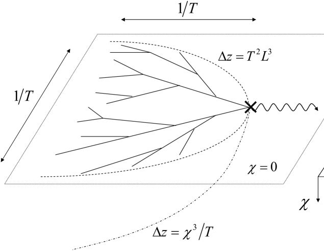
Figure 25: The parton cascade generated by the current via medium–induced branching in the physical Minkowski space (represented here as the boundary of $AdS_{5}$ at $\chi=0$) and the trailing string attached to the leading photon (represented for $\chi\ll 1$). The latter is ‘dual’ to the enveloping curve of the former.

As another check of this physical interpretation, let us compare the ‘drag force’ computed in Refs. [32, 33] — the force which is required to pull the heavy quark at constant speed through the plasma — to the rate of energy degradation for partons in our parton cascade. (In the case of the heavy quark, this is also the rate at which the heavy quark looses energy, since this quark can be traced during the branching process, due to its conserved baryonic charge.) Namely, in Refs. [32, 33] one found

$$-\,\frac{{\rm d}E}{{\rm d}t}\,=\,\frac{\pi}{2}\sqrt{\lambda}\,v_{z}^{2}\,\gamma\,T^{2}\,,$$ (5.104)

with $v_{z}$ the (constant) velocity of the heavy quark and $\gamma=1/\sqrt{1-v^{2}_{z}}$. On the other hand, for the branching process described in this section we can write (this follows from Eq. (5.95) by using $\omega(t)\sim Q^{3}(t)/T^{2}$, or directly from Eq. (5.99))

$$-\,\frac{{\rm d}\omega(t)}{{\rm d}t}\,\sim\,Q_{s}^{2}(\omega(t),T)\,\sim\,(\omega(t)T^{2})^{2/3}\,\sim\,\gamma(t)T^{2}\,.$$ (5.105)

where $\gamma(t)=\omega(t)/Q(t)$ is now time-dependent, because we are not in a stationary situation (there is no drag force). But except for this time–dependence, Eqs. (5.104) and (5.105) are indeed consistent with each other : in both cases, the rate for energy loss is proportional to $\gamma T^{2}$.

What happens with this energy after being transferred to the plasma, i.e., at times $t>t_{f}$ (corresponding to large distances $L,\,\zeta>1/T$) ? This question cannot be answered on the basis of the branching picture alone, nor within our previous approximations for the supergravity solution, which are valid only sufficiently far away from the horizon. The proper answer to this question within AdS/CFT would require a more precise solution, valid near the horizon, and also a study of the backreaction of the Maxwell wave on the $AdS_{5}$ BH geometry [68, 69]. Such a study has not been done so far for the problem of the $\mathcal{R}$–current, but similar analyses for the ‘heavy quark’ problem [37, 38] show that the transfer of energy from the hard probe to the plasma induces collective motion in the latter, in the form of sound waves or Mach cones.

5.4 Physical interpretation: Parton saturation at strong coupling

We now return to the AdS/CFT results for a space–like current, cf. Sect. 5.1, and show that these can be naturally interpreted in terms of parton distributions in the strongly–coupled plasma. From Sect. 2.2 we recall that the structure function $F_{2}(x,Q^{2})$ is a measure of the hadron (here, plasma) constituents with longitudinal momentum fraction $x$ and transverse momenta $k_{\perp}\lesssim Q$ (i.e., which occupy a transverse area $\sim 1/Q^{2}$). Hence, by inspection of the corresponding results in Sect. 5.1, one can immediately deduce that there are no partons at sufficiently large values of $Q^{2}\gg Q^{2}_{s}(x)=(T/x)^{2}$ for a given value of $x$, or, equivalently, at sufficiently large values of $x$ for a given $Q^{2}$. Indeed, the structure functions are exponentially suppressed in this high–$Q^{2}$ (or ‘low–energy’, or ‘large–$x$’) regime, as shown in Eq. (5.78) that one can rewrite as

$$F_{2}/(x{N^{2}_{c}Q^{2}})\,\sim\,\exp\big{\{}-c(Q/Q_{s})^{1/2}\big{\}}\,=\,\exp\big{\{}-c(x/x_{s})^{1/2}\big{\}}\quad{\rm for}\quad x>x_{s}\equiv\frac{T}{Q}\,.$$ (5.106)

The saturation line $Q_{s}(x)=T/x$ is shown as the straight line $\ln Q_{s}^{2}(Y)=2Y$ in the kinematical plane for DIS, in Fig. 26 left. As also indicated in that figure, there are no partons on the right side of the saturation line: the respective structure functions are so small that the scattering can be characterized as quasi–elastic. The absence of partons from the wavefunction of a hadron at strong coupling (and for relatively large $Q^{2}$) was anticipated by Polchinski and Strassler [51], via the following argument based on the operator product expansion (OPE) :

   

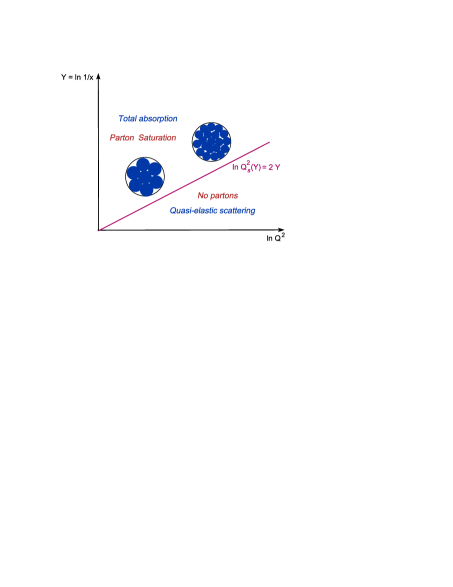
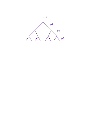
Figure 26: Left: The ‘phase diagram’ for DIS off a ${\mathcal{N}}=4$ SYM plasma at high energy and strong coupling. Right: Parton cascades through which the partons fall at small values of $x\lesssim x_{s}$.

At weak coupling, the parton picture for DIS is meaningful because the OPE for the structure functions at high $Q^{2}$ is dominated by the operators with leading twist — i.e., those having the minimal value for the difference $\tau_{j,n}\equiv\Delta_{j,n}-j$ between their mass dimension $\Delta_{j,n}$ and their spin $j$ ($n$ is an operator index) —, which have a manifest interpretation in terms of quark and gluon number densities (see, e.g., [58]). In the classical, or zero–order, approximation, this value is $\tau_{\rm cl}=2$ for all the ‘leading–twist’ operators. But in general this classical value receives quantum corrections in the form of the ‘anomalous dimensions’ $\gamma_{j,n}\equiv\Delta_{j,n}-d_{j,n}$ (with $d_{j,n}$ the respective classical dimension). At weak coupling, these anomalous dimensions start at $\mathcal{O}{(g^{2})}$ and can be computed in perturbation theory; in particular, for a theory with conformal symmetry, so like the ${\mathcal{N}}=4$ SYM theory, and for large $N_{c}$, these are pure numbers $\gamma_{j,n}\sim g^{2}N_{c}\equiv\lambda$ which turn out to be positive, or zero in some exceptional cases. The ‘exceptional cases’ refer to the operators which are ‘protected’ against quantum corrections by some symmetry, so like the energy–momentum tensor $T^{\mu\nu}$ (for which $j=2$ and $\gamma=0$). The fact that $\gamma_{j,n}$ is positive means that the respective contribution to the OPE of $F_{2}(x,Q^{2})$ decreases with increasing $Q^{2}$, according to the power law $(1/Q^{2})^{\gamma_{j,n}/2}$. (In pQCD, due to asymptotic freedom, this decrease is slower, as an inverse power of $\ln Q^{2}$ [58].) But at weak coupling, the exponent $\gamma_{j,n}/2\sim g^{2}N_{c}\ll 1$ is small, so in spite of their positive anomalous dimensions the ‘leading–twist’ operators still dominate over those with a higher (classical) twist $\tau\geq 3$.

The situation however changes when moving to strong coupling, as Polchinski and Strassler have emphasized: there, the anomalous dimensions for the leading–twist operators are very large, of $\mathcal{O}{(\lambda^{1/4})}$ [76], and they are still positive (whenever non–vanishing), so the respective contributions die away very fast with increasing $Q^{2}$. As a consequence, the DIS structure functions at high $Q^{2}$ and strong coupling are rather dominated by special higher–twist operators which are protected by symmetries, and which in general can be of two types: operators which describe the scattering off the hadron as a whole [51] (as opposed to the scattering off its partonic constituents), and multiple insertions of the protected leading–twist operator $T^{\mu\nu}$, which can be interpreted as diffractive scattering [52]. (In the dual string theory, such diffractive processes appear as multiple graviton exchanges which can be resummed in the eikonal approximation [78, 79].) These higher–twist operators provide contributions to $F_{2}(x,Q^{2})$ which at high $Q^{2}$ fall off as large, but finite (i.e., independent of $\lambda$), powers of $1/Q^{2}$.

Yet, for the strongly–coupled plasma, the structure functions in Eq. (5.106) show an even faster decrease at high $Q^{2}$ — exponential rather than power–like. This is so since these results correspond to the strict limit $N_{c}\to\infty$, in which the multiple graviton exchanges with a single constituent of the plasma are naturally suppressed: indeed, each such an exchange is of order $1/N_{c}^{2}$; this suppression can be compensated by the large number $\propto N^{2}_{c}$ of degrees of freedom in the plasma (this explains why the potential for one–graviton–exchange in Eq. (5.77) is independent of $N_{c}$), but this is not possible when the scattering involves only a single constituent of the plasma. This explains why the plasma structure functions have no power tail at high $Q^{2}$. As for the fact that this tail is exponential, this can be understood as follows: In the previous subsection, we have argued that the gravitational interactions in the supergravity problem correspond, in the dual gauge theory, to a constant force $F_{T}\sim T^{2}$ acting on a colored particle within the plasma. Then the plasma–induced decay of a space–like current with high $Q^{2}$ can be understood as a version of the Schwinger mechanism for pair production by a uniform electric field.

We now turn to the more interesting case at small–$x$, $x\lesssim x_{s}=T/Q$, or relatively small virtuality $Q^{2}\lesssim Q_{s}^{2}$, where the plasma structure functions are significantly large, cf. Eq. (5.86), which is suggestive of a parton picture. To develop such a picture, we need two additional ingredients:

(i) The Breit frame
Recall that the concept of ‘parton’ makes sense only in a frame in which the plasma has a large longitudinal momentum (an ‘infinite momentum frame’). It is convenient to choose the Breit frame, which is the frame in which the $\mathcal{R}$–current is a standing wave, with 4–momentum $q^{\prime\mu}=(0,0,0,Q)$. This frame is obtained from the plasma rest frame by performing a boost in the negative $z$ direction with a boost factor equal to that of the original current, i.e., $\gamma=k/Q$. A typical quanta in the plasma (whatever is its nature) has energy and momentum of order $T$ in the plasma rest frame, hence it will have a longitudinal momentum $\sim\gamma T$ in the Breit frame. However the current is not absorbed directly by such a typical, thermal, quanta, rather by a partonic constituent of it, which carries only a small fraction $x=Q^{2}/(2\omega T)\ll 1$ of its longitudinal momentum; hence, this parton has a longitudinal momentum $p^{\prime}_{z}\sim x(\gamma T)\simeq Q$. We see that, in this particular frame, the current acts as a probe of the plasma with both longitudinal and transverse resolutions equal to $Q$.

(ii) The energy sum rule
We have previously mentioned the fact that the spin–2 operator $T^{\mu\nu}$ receives no anomalous dimension, because of energy–momentum conservation. This can be used to demonstrate the sum–rule (2.22) for the longitudinal momentum fraction inside a hadron wavefunction [58]: this sum–rule is proportional to the expectation value $\langle T^{\mu\nu}\rangle$, and hence it is independent of $Q^{2}$. There are similar sum–rules constraining the plasma structure functions [30]; for instance,

$$\mathcal{E}\,=\,18T^{2}\int_{0}^{1}{\rm d}x\,F_{2}(x,Q^{2})\,,$$ (5.107)

where $\mathcal{E}$ is the energy density in the ${\mathcal{N}}=4$ SYM plasma at infinite coupling:

$$\mathcal{E}\,\equiv\,\langle T^{00}\rangle\,=\,\frac{3\pi^{2}}{8}\,N^{2}_{c}T^{4}\,.$$ (5.108)

Let us first check that Eq. (5.107) is indeed verified, at least parametrically, by our present approximation for $F_{2}$. Clearly, the region at (relatively) large $x\gg x_{s}$ yields only a negligible contribution to the integral, since $F_{2}$ is exponentially suppressed there. Using Eq. (5.86) for $x\lesssim x_{s}=T/Q$, one can check that the integral is in fact dominated by the upper limit $x\simeq x_{s}$ of this ‘small–$x$’ region, i.e., by points in the vicinity of the saturation line; moreover, these points yield a contribution with the right order of magnitude: $T^{2}\,xF_{2}(x,Q^{2})\sim N_{c}^{2}T^{4}$ for $x\sim T/Q$ (for any $Q^{2}$ !). Note that, with increasing $Q^{2}$, the support of the structure function $F_{2}(x,Q^{2})$ shrinks to smaller and smaller values of $x\lesssim T/Q$ (cf. Fig. 26 left).

One can furthermore rely on Eq. (5.107) to deduce a physical interpretation for $F_{2}(x,Q^{2})$ valid in the Breit frame. In this frame, the energy density reads $\mathcal{E}^{\prime}=\gamma^{2}\mathcal{E}$ and the current explores a region of the plasma with longitudinal width $\Delta z^{\prime}\sim 1/Q$. Note that $\Delta z^{\prime}$ is the same as the coherence time of the current, cf. Eq. (4.61), when measured in the Breit frame. Hence, the quantity

$$\frac{{\rm d}E^{\prime}}{{\rm d}^{2}b}\,\equiv\,\mathcal{E}^{\prime}\times\Delta z^{\prime}\,\sim\,\gamma\times\frac{\gamma}{Q}\times\mathcal{E}$$ (5.109)

represents the energy per unit transverse area in the region of the plasma explored by the current. Using ${\gamma}/{Q}\sim 1/(xT)$ together with Eq. (5.107), we deduce

$$\frac{{\rm d}E^{\prime}}{{\rm d}^{2}b}\sim xT\gamma\left(\frac{1}{x}\,F_{2}(x,Q^{2})\right)_{x=T/Q}\,.$$ (5.110)

As before mentioned, the quantity $xT\gamma\sim Q$ in the r.h.s. is the longitudinal momentum of the constituent (parton) which interacts with the ${\mathcal{R}}$–current. It is therefore natural to interpret

$$\frac{1}{x}\,F_{2}(x,Q^{2})\Big{|}_{x=T/Q}\sim\frac{{\rm d}N}{{\rm d}Y{\rm d}^{2}b_{\perp}}\Big{|}_{x=T/Q}\,,$$ (5.111)

as the number of partons in the plasma per unit area per unit rapidity as ‘seen’ by a virtual photon with resolution $Q$. The occurrence of the rapidity $Y\equiv\ln(1/x)$ can be understood in the same as way as for the hadron structure functions in Sect. 2.2 (cf. Eq. (2.24)): namely, the partons explored by the virtual photon have longitudinal momentum $p^{\prime}_{z}\sim Q$ and occupy a longitudinal distance $\Delta z^{\prime}\sim 1/Q$, hence they are distributed within one unit of rapidity: $\Delta Y=\Delta z^{\prime}\Delta p^{\prime}_{z}\sim 1$.

On the other hand, the AdS/CFT calculation in Sect. 5.1 implies, cf. Eq. (5.86),

$$\frac{1}{x}\,F_{2}(x,Q^{2})\Big{|}_{x=T/Q}\,\sim\,N_{c}^{2}Q^{2}\qquad\mbox{for}\qquad x\sim T/Q\,.$$ (5.112)

By comparing Eqs. (5.111) and (5.112), we finally deduce

$$\frac{{\rm d}N}{{\rm d}Y{\rm d}^{2}b_{\perp}}\,\equiv\,\int^{Q}\!\!{\rm d}^{2}k_{\perp}\ \frac{{\rm d}N}{{\rm d}Y{\rm d}^{2}b_{\perp}{\rm d}^{2}k_{\perp}}\,\sim\,N_{c}^{2}Q^{2}\qquad\mbox{for}\qquad x\sim T/Q\,.$$ (5.113)

This result is naturally interpreted as saying that the partons with $x\sim T/Q$ are distributed in phase–space in such a way that, at all transverse momenta $k_{\perp}\lesssim Q$, there is roughly one parton of each color per unit phase–space. Alternatively, one can say that, for a given value of $x\ll 1$, the partons occupy the phase–space on the left of the saturation line, i.e., at $k_{\perp}\lesssim Q_{s}(x)=T/x$, with occupation numbers of $\mathcal{O}{(1)}$ :

$$\frac{1}{N^{2}_{c}}\,\frac{{\rm d}N}{{\rm d}Y{\rm d}^{2}b_{\perp}{\rm d}^{2}k_{\perp}}\,\simeq\,1\qquad\mbox{for}\qquad k_{\perp}\lesssim Q_{s}(x)\,=\,\frac{T}{x}\,.$$ (5.114)

This phase–space distribution is reminiscent of that produced by gluon saturation in weakly–coupled QCD (cf. Sect. 2.1 and Fig. 16) — the occupation numbers are maximal and uniform (i.e., independent of $Y$ and $k_{\perp}$) on the left of the saturation line, and they decrease rapidly when moving to its right — but there are also interesting differences: (i) the occupation numbers at saturation are of $\mathcal{O}{(1)}$ at strong coupling, while they were much larger, $\sim{1/\lambda}\gg 1$, in the perturbative regime at $\lambda\ll 1$; (ii) in the dilute region at $k_{\perp}\gg Q_{s}(x)$ there are essentially no partons in the strongly–coupled plasma, while in pQCD the respective occupation numbers decrease rather slowly, roughly like $(Q_{s}/k_{\perp})^{2}$ (cf. Eq. (2.26)); (iii) for a given, ‘hard’, resolution $Q^{2}$, the energy of a hadron in pQCD is carried mostly by its large–$x$ partons, while at strong coupling this is rather concentrated in the vicinity of the saturation line, i.e., at small $x$; (iv) the rise of the saturation momentum with $1/x$ is much faster at strong coupling than at weak coupling: the saturation exponent $\omega_{s}$ (introduced in Eq. (2.27)) is estimated as $\omega_{s}\sim 0.2\div 0.3$ in pQCD, and as $\omega_{s}=2$ for the strongly–coupled plasma (cf. Eq. (5.80)).

The fact that, at strong coupling, all partons lie at small values of $x$ is in fact quite natural [51, 52], and can be heuristically explained via the ‘quasi–democratic branching’ scenario previously introduced for the ${\mathcal{R}}$–current (cf. Sect. 4.4). Already at weak coupling, we noticed in Sect. 2.2 the natural tendency of the parton evolution to increase the number of partons with small values of $x$. In that case, however, the evolution was biased towards the emission of small–$x$ gluons, which carry only a small fraction $x\ll 1$ of the longitudinal momentum of their parent parton; hence, after emission, the latter could emerge with a relatively large momentum, which explains why most of the total energy was still carried by the large–$x$ partons. By contrast, at strong coupling there is no reason why the energy and momentum should not be ‘democratically’ divided among the daughter partons. Then the energy is rapidly degraded along the parton cascade (as illustrated in Fig. 26 right), and no partons can survive at large $x$. The fact that this branching process stops when $x$ becomes as small as $x_{s}\sim T/Q$ can be ‘understood’ as a consequence of energy conservation, Eq. (5.107), together with the condition that the occupation numbers at strong coupling cannot be much larger than one. However, we have no intuitive explanation for this last condition, except for the fact that it looks natural.

Note that there is nothing specific to the finite–temperature plasma in the above argument, and indeed it turns out that a similar partonic picture holds also for a single hadron at strong coupling. This was studied in Refs. [51, 52], with the ‘hadron’ being a bound state (a kind of glueball) of the ${\mathcal{N}}=4$ SYM theory ‘deformed’ by the introduction of an infrared cutoff $\Lambda$, to mimic confinement. Via AdS/CFT, this ‘glueball’ is dual to a dilaton state in supergravity. The respective DIS process is then computed as the graviton–mediated scattering between the dilaton and the Maxwell wave induced in $AdS_{5}$ by the ${\mathcal{R}}$–current. For sufficiently high $Q^{2}$, the inelastic scattering is mainly ‘diffractive’ — it proceeds via multiple graviton exchanges —, and its study requires going beyond the classical supergravity approximation — in the sense that $N_{c}$ must be kept finite, although large, to allow for multiple scattering. (The large–$N_{c}$ limit and the high–energy limit are then correlated with each other [52].) The main conclusion in Ref. [52] is that the hadron wavefunction at strong coupling can be given a partonic interpretation which is quite similar to that for the plasma: all partons are concentrated, with occupation numbers of $\mathcal{O}{(1)}$, at transverse momenta below the respective saturation momentum, which reads

$$Q_{s}^{2}(x)\,=\,\frac{\Lambda^{2}}{xN_{c}^{2}}\qquad\mbox{(hadron at strong coupling)}\,.$$ (5.115)

This is suppressed in the large $N_{c}$ limit since so is the scattering amplitude. (In the case of the plasma, this suppression is compensated by the number of thermal degrees of freedom, which is proportional to $N_{c}^{2}$.) The fact that $Q_{s}^{2}(x)$ rises as $1/x$ is the expected ‘Regge behaviour’ $\propto 1/x^{j-1}$ for an amplitude mediated by the exchange of a ‘particle’ with spin $j$ — here, a graviton with $j=2$. The corresponding rise appears to be even faster in the case of the plasma, where we have seen that $Q_{s}^{2}(x)=T^{2}/x^{2}$ (cf. Eq. (5.80)). This difference can be easily understood: $Q_{s}^{2}(x)$ is proportional to the density of partons per unit transverse area, as obtained after integrating over the longitudinal extent of the interaction region (recall, e.g., Eq. (2.26)). For a hadron, this longitudinal extent is simply the hadron width, and is independent of $x$. But for the plasma this is set by the coherence time of the virtual photon, that is, $\Delta t_{\rm coh}\sim 1/xT$ (cf. Eq. (4.61)); this explains the additional factor of $1/x$ in Eq. (5.80).

The above argument also suggests an heuristic way to generalize our previous results to a plasma with finite longitudinal extent (a situation which may be relevant to phenomenology): Namely, so long as this extent is much larger than the photon coherence time, then everything proceeds like for an infinite plasma, and the saturation momentum is given by Eq. (5.80). On the other hand, if the plasma has a longitudinal width $L_{z}\ll\Delta t_{\rm coh}$, the corresponding value for $Q_{s}^{2}$ can be obtained by rescaling the result in Eq. (5.80) by a factor $L_{z}/\Delta t_{\rm coh}\sim xTL_{z}$. This yields

$$Q_{s}^{2}(x,T,L_{z})\,\sim\,\frac{T^{3}L_{z}}{x}\qquad\mbox{(plasma with longitudinal extent $L_{z}\ll 1/xT$)}\,.$$ (5.116)

A more detailed argument supporting this conclusion will be presented in the Appendix.

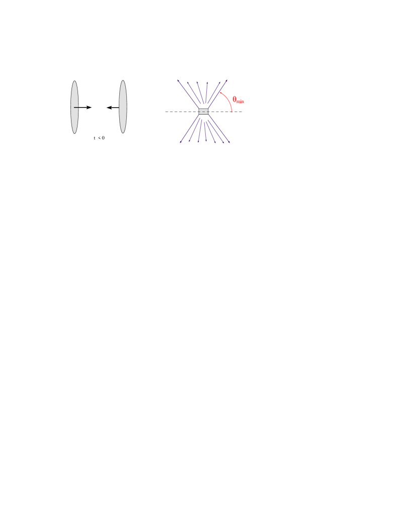
Figure 27: A picture of a hypothetical hadron–hadron collision at strong coupling: there is no particle production within an angle $\theta_{\rm min}$ around the collision axis, which is determined by $x_{s}$.

The peculiar partonic picture has striking consequences for a (hypothetical) nucleus–nucleus collision at strong coupling. Such a collision allows us to visualise the partons in the incoming nuclear wavefunctions: they are first liberated by the collision and then hadronise on their way towards the detector. Those hadrons originating in large–$x$ partons have large longitudinal momenta and thus appear in the detector at either forward, or backward, ‘rapidities’, i.e., at small angles relative to the collision axis. (Here, by ‘rapidity’ we mean the space–time rapidity $\eta$ related to the collision angle by $\eta=-\ln\tan({\theta}/{2})$; for a massless particle, $\eta$ coincides with the momentum rapidity.) By contrast, the small–$x$ partons give rise to hadrons which appear at ‘central rapidities’ $\eta\approx 0$, i.e., at large scattering angles $\theta\simeq\pi/2$. In the actual $AA$ collisions at RHIC, one clearly sees the hadrons being produced at both forward, and central, rapidities, and the latter are more numerous than the former. This observation is in agreement with the parton balance in the nuclear wavefunction as predicted by pQCD (cf. Sect. 2.2). But the situation would be very different at strong coupling: the absence of large–$x$ partons in the incoming wavefunction would then imply that there is no particle production at small angles, so the final event would exhibit ‘rapidity gaps’ $\eta_{\rm gap}(Q)\simeq\ln(1/x_{s}(Q))$ (for jets with transverse momentum $Q$) in both forward and backward directions (see Fig. 27).

6 Concluding remarks

The main lesson of these lectures may be summarized as follows: The physical picture of a plasma as revealed by hard probes and, more generally, the overall picture of scattering at high energy appear to be quite different at strong coupling as compared to the respective predictions of perturbative QCD, and also to the actual experimental observations. At strong coupling, there are no jets in $e^{+}e^{-}$ annihilation, no forward/backward particle production in hadron–hadron collisions, no partons in the hadron wavefunctions except at very small $x$. Also, phenomena like the energy loss or the transverse momentum broadening of a partonic jets travelling into the plasma are controlled by different mechanisms at strong coupling — where, as we have seen, the dominant mechanism at work is medium–induced parton branching —, as compared to weak coupling — where the momentum broadening is mainly due to thermal rescattering, and the energy loss to the emission of a hard gluon (as made possible by thermal rescattering, once again) [81, 82, 8].

Such differences should not come as a surprise: they reflect the fact that the corresponding processes involve large momentum transfers, so in QCD they are naturally controlled by small values of the coupling, because of asymptotic freedom. Accordingly, much caution should be taken when trying to extrapolate results from AdS/CFT to QCD in this particular context of high–energy scattering and hard probes. But this does not exclude the possibility that long–range processes in the quark–gluon plasma (so like transport and screening phenomena, or the approach towards thermalization) be still strongly coupled, precisely because they involve smaller energies and momenta. This may explain the RHIC data for elliptic flow which, as explained in the Introduction, are consistent with a small value for the viscosity–to–entropy ratio, as expected for a strongly–interacting fluid. For a theory with asymptotic freedom and confinement, so like QCD, it is natural and necessary to use different effective theories (or descriptions) at different energy–momentum scales, as well known from the experience with nuclear theory, chiral perturbation theory, heavy–quark effective theory, hard thermal loops, color glass condensate, etc. From this perspective, the gauge/gravity duality is so far the unique effective theory which allows us to address long–range and time–dependent phenomena in a QCD–like plasma in the regime of strong coupling. This method has already produced some very interesting results, so like the lower bound on the $\eta/s$ ratio mentioned in the Introduction, and has the potential to explain some outstanding open questions, so like the rapid thermalization of the quark–gluon matter observed at RHIC, which seem to transcend perturbation theory. This is explained in the lecture notes by M. Heller, R. Janik and R. Peschanski, included in this volume [83].

But even in the context of hard probes, which has been our main concern throughout these lectures, the gauge/gravity duality may turn out to be useful. Some of the observables measured by hard probes (so like jet quenching) receive contributions from both short–range and long–range phenomena, and thus combine perturbative and non–perturbative aspects. A possible strategy to deal with such phenomena, as suggested in Refs. [84, 85], is to distinguish between the respective ‘hard’ and ‘soft’ momentum contributions, and then use string–inspired techniques in the soft sector alone, while the hard sector is still treated in perturbation theory.

Acknowledgments

I would like to thank the organizers of the 48th Cracow School of Theoretical Physics Aspects of Duality for their warm hospitality at Zakopane during the School and for their patience with my slow writing of these lectures notes. I am grateful to Al Mueller for suggestions on the manuscript (in particular, for the argument developed in Appendix) and to Grégory Giecold for a careful reading. This work is supported in part by Agence Nationale de la Recherche via the programme ANR-06-BLAN-0285-01.

Appendix A Saturation momentum for a finite–size plasma

Towards the end of Sect. 5 we have conjectured a formula, Eq. (5.116), for the saturation momentum of a plasma whose longitudinal extent $L_{z}$ is smaller than the coherence length ${\omega}/{Q^{2}}$ of the incoming virtual photon. In this Appendix, we shall present an argument based on the previous AdS/CFT calculations which supports this formula. This requires a more precise identification of the physical force acting on the virtual photon in the strongly coupled plasma, and thus is a little ambiguous — it involves subtle differences of physical interpretation which cannot be fully justified without an explicit calculation.

As discussed in Sect. 5.3, the physical transverse force exerted by the plasma can be identified, via the UV/IR correspondence, with the attraction exerted by the black hole on the Maxwell wave. For definiteness, we focus on the high-energy case $\omega\gtrsim Q^{3}/T^{2}$, where the virtuality drops out from the potential felt by the Maxwell wave. Then, as explained after Eq. (5.81), the radial fall of the wave–packet at late times can be described as the motion of a classical particle in the potential $V\simeq V_{c}$. The corresponding Newton law is shown in Eq. (5.82), which can be rewritten as

$$k\,\frac{{\rm d}^{2}\chi}{{\rm d}t^{2}}\,=\,2k\,\frac{\chi^{3}}{\chi_{0}^{4}}\,.$$ (A.117)

Via the UV/IR correspondence $\chi\sim L$, this is naturally interpreted as a transverse force acting on the virtual photon (or, more precisely, on its partonic fluctuation) in the plasma:

$$F_{T}\,\equiv\,k\ddot{L}\,\sim\,kL^{3}T^{4}\,\sim\,T^{3}\,\frac{L}{x}\,,$$ (A.118)

where the last estimate follows after recalling that $L\sim 1/Q$ (by the uncertainty principle) and $x\sim Q^{2}/kT$. The emergence of the longitudinal momentum $k$ as an inertial mass for the transverse dynamics is natural for a classical particle moving with very high momentum.

Eq. (A.118) is the most general prediction of the present AdS/CFT calculation for the plasma force. One might interpret the various factors in this equation as follows: $T^{3}$ is the density of thermal excitations in the plasma, $L$ (the transverse size of the partonic fluctuation) appears because this is a dipolar force, and $1/x$ reflects the scattering via graviton exchange. For the case of the infinite plasma, Eq. (A.118) is equivalent with the force $F_{T}\sim T^{2}$ argued in Sect. 5.3. For instance, it gives rises to the same estimate for the saturation momentum, Eq. (5.80), as we show now: In the infinite plasma, a space–like current interacts with the medium over a time $\Delta t_{\rm coh}\sim{\omega}/{Q^{2}}\sim 1/xT$; for the current to decay, it must receive a mechanical work $F_{T}\times\Delta t_{\rm coh}$ from the plasma that compensate for its virtuality. This condition implies

$$T^{3}\,\frac{1}{xQ}\times\frac{1}{xT}\,\sim\,Q\ \Longrightarrow\ Q^{2}\,\sim\,Q_{s}^{2}(x,T)\,\equiv\,\frac{T^{2}}{x^{2}}\,.$$ (A.119)

Furthermore, in the high–energy regime, the effective virtuality of the current is set by the saturation momentum (since the maximal size of its partonic fluctuation is $1/Q_{s}\ll 1/Q$). With $L\sim 1/Q_{s}=x/T$, Eq. (A.118) yields $F_{T}\sim T^{2}$, as anticipated.

On the other hand for a finize–size medium, with longitudinal extent $L_{z}\lesssim\Delta t_{\rm coh}$, the mechanical work is $F_{T}\times L_{z}$, and the saturation condition becomes

$$T^{3}\,\frac{1}{xQ}\times L_{z}\,\sim\,Q\ \Longrightarrow\ Q^{2}\,\sim\,Q_{s}^{2}(x,T,L_{z})\,\equiv\,\frac{T^{3}L_{z}}{x}\,,$$ (A.120)

in agreement with Eq. (5.116).

What is particularly appealing about Eq. (A.118) is that it exhibits the $1/x$ rise at high–energy associated with one graviton exchange, whose appearance is natural in the context of the supergravity calculation, but which remains a bit mysterious back in the original gauge theory.

References

- [1] I. Arsene et al. [BRAHMS Collaboration], Nucl. Phys. A757 (2005) 1.
- [2] B. B. Back et al. [PHOBOS Collaboration], Nucl. Phys. A757 (2005) 28 [arXiv:nucl-ex/0410022].
- [3] J. Adams et al. [STAR Collaboration], Nucl. Phys. A757 (2005) 102 [arXiv:nucl-ex/0501009].
- [4] K. Adcox et al. [PHENIX Collaboration], Nucl. Phys. A757 (2005) 184 [arXiv:nucl-ex/0410003].
- [5] E. Shuryak, “Why does the quark gluon plasma at RHIC behave as a nearly ideal fluid?”, Prog. Part. Nucl. Phys. 53 (2004) 273; “Physics of Strongly coupled Quark-Gluon Plasma,” arXiv:0807.3033 [hep-ph].
- [6] M. Gyulassy and L. McLerran, “New forms of QCD matter discovered at RHIC”, Nucl. Phys. A 750 (2005) 30.
- [7] B. Muller, “From Quark-Gluon Plasma to the Perfect Liquid”, Acta Phys. Polon. B38 (2007) 3705, arXiv:0710.3366 [nucl-th].
- [8] J. Casalderrey-Solana and C. A. Salgado, Acta Phys. Polon. B38 (2007) 3731, arXiv:0712.3443 [hep-ph].
- [9] U. W. Heinz, “The strongly coupled quark-gluon plasma created at RHIC,” arXiv:0810.5529 [nucl-th].
- [10] J. M. Maldacena, Adv. Theor. Math. Phys. 2 (1998) 231.
- [11] S. S. Gubser, I. R. Klebanov, and A. M. Polyakov, Phys. Lett. B428 (1998) 105.
- [12] E. Witten, Adv. Theor. Math. Phys. 2 (1998) 505.
- [13] O. Aharony, S. S. Gubser, J. M. Maldacena, H. Ooguri, and Y. Oz, “Large N field theories, string theory and gravity”, Phys. Rept. 323 (2000) 183.
- [14] D. T. Son and A. O. Starinets, “Viscosity, Black Holes, and Quantum Field Theory,” Ann. Rev. Nucl. Part. Sci. 57 (2007)95 0704.0240 [hep-th].
- [15] J. Y. Ollitrault, Phys. Rev. D46 (1992) 229.
- [16] G. Policastro, D. T. Son and A. O. Starinets, Phys. Rev. Lett. 87 (2001) 081601; JHEP 0209 043; JHEP 0212 (2002) 054.
- [17] P. Kovtun, D. T. Son and A. O. Starinets, Phys. Rev. Lett. 94 (2005) 111601.
- [18] D. Teaney, Phys. Rev. C68 (2003) 034913.
- [19] M. Luzum and P. Romatschke, Phys. Rev. C78 (2008) 034915.
- [20] K. J. Eskola, H. Honkanen, C. A. Salgado and U. A. Wiedemann, Nucl. Phys. A747 (2005) 511.
- [21] A. Dainese, C. Loizides and G. Paic, Eur. Phys. J. C38 (2005) 461.
- [22] R. Baier and D. Schiff, JHEP 0609 (2006) 059
- [23] M. Cheng et al. [RBC-Bielefeld Collaboration], Phys. Rev. D77 014511 (2008).
- [24] F. Karsch, E. Laermann and A. Peikert, Phys. Lett. B 478 (2000) 447.
- [25] J.-P. Blaizot, E. Iancu, A. Rebhan, Phys. Rev. Lett. 83 (1999) 2906; Phys. Rev. D63 065003 (2001).
- [26] S. S. Gubser, I. R. Klebanov and A. A. Tseytlin, Nucl. Phys. B534 (1998) 202.
- [27] M. A. Vazquez-Mozo, Phys. Rev. D60 (1999) 106010.
- [28] J.-P. Blaizot, E. Iancu, A. Rebhan, JHEP 06 (2007) 035.
- [29] J.-P. Blaizot, E. Iancu, Phys. Rept. 359 (2002) 355; J.-P. Blaizot, E. Iancu, A. Rebhan, hep-ph/0303185; U. Kraemmer, A. Rebhan, Rept. Prog. Phys. 67 (2004) 351.
- [30] Y. Hatta, E. Iancu, and A. H. Mueller, JHEP 0801 (2008) 063.
- [31] Y. Hatta, E. Iancu, and A. H. Mueller, JHEP 0805 (2008) 037.
- [32] C. P. Herzog, A. Karch, P. Kovtun, C. Kozcaz, and L. G. Yaffe, JHEP 0607 (2006) 013.
- [33] S. S. Gubser, Phys. Rev. D74 (2006) 126005.
- [34] J. Casalderrey-Solana and D. Teaney, JHEP 04 (2007) 039; Phys. Rev. D74 (2006) 085012.
- [35] S. S. Gubser, Nucl. Phys. B790 (2008) 175.
- [36] J. J. Friess, S. S. Gubser, G. Michalogiorgakis and S. S. Pufu, Phys. Rev. D75 (2007) 106003.
- [37] S. S. Gubser, S. S. Pufu, and A. Yarom, JHEP 09 (2007) 108.
- [38] P. M. Chesler and L. G. Yaffe, Phys. Rev. Lett. 99 (2007) 152001; Phys. Rev. D78 (2008) 045013
- [39] F. Dominguez, C. Marquet, A.H. Mueller, Bin Wu, Bo-Wen Xiao, Nucl. Phys. A811 (2008) 197.
- [40] M. Kruczenski, D. Mateos, R. C. Myers and D. J. Winters, JHEP 0307 (2003) 049.
- [41] K. Peeters, J. Sonnenschein, and M. Zamaklar, Phys. Rev. D74 (2006) 106008.
- [42] H. Liu, K. Rajagopal, and U. A. Wiedemann, Phys. Rev. Lett. 98 (2007) 182301.
- [43] M. Chernicoff, J. A. Garcia, and A. Guijosa, JHEP 0609 (2006) 068.
- [44] E. Caceres, M. Natsuume, and T. Okamura, JHEP 0610 (2006) 011.
- [45] Q. J. Ejaz, T. Faulkner, H. Liu, K. Rajagopal and U. A. Wiedemann, JHEP 0804 (2008) 089.
- [46] R. C. Myers and A. Sinha, JHEP 0806 (2008) 052.
- [47] T. Faulkner and H. Liu, “Meson widths from string worldsheet instantons,” arXiv:0807.0063 [hep-th].
- [48] S. S. Gubser, D. R. Gulotta, S. S. Pufu, and F. D. Rocha, arXiv:0803.1470 [hep-th].
- [49] P.M. Chesler, K. Jensen, and A. Karch, arXiv:0804.3110 [hep-th].
- [50] P. M. Chesler, K. Jensen, A. Karch and L. G. Yaffe, “Light quark energy loss in strongly-coupled N = 4 supersymmetric Yang-Mills plasma”, arXiv:0810.1985 [hep-th].
- [51] J. Polchinski and M. J. Strassler, JHEP 0305 (2003) 012.
- [52] Y. Hatta, E. Iancu, and A. H. Mueller, JHEP 0801 (2008) 026.
- [53] A.H. Mueller, “Parton Saturation–An Overview”, hep-ph/0111244; E. Iancu, A. Leonidov and L. McLerran, “The Colour Glass Condensate: An Introduction”, hep-ph/0202270; E. Iancu and R. Venugopalan, “The Color Glass Condensate and High Energy Scattering in QCD”, hep-ph/0303204; H. Weigert, “Evolution at small : The Color Glass Condensate”, hep-ph/0501087; J. Jalilian–Marian and Y. Kovchegov, “Saturation Physics and Deuteron–Gold Collisions at RHIC”, hep-ph/0505052.
- [54] K. Becker, M. Becker and J. H. Schwarz, “String theory and M-theory: A modern introduction,” Cambridge, UK: Cambridge Univ. Pr. (2007) 739 p.
- [55] E. Kiritsis, “String theory in a nutshell,” Princeton, USA: Univ. Pr. (2007) 588 p.
- [56] L. Susskind and E. Witten, “The holographic bound in anti-de Sitter space,” hep-th/9805114. A. W. Peet and J. Polchinski, Phys. Rev. D59 (1999) 065011.
- [57] S. J. Brodsky and G. F. de Teramond, “AdS/CFT and Light-Front QCD”, arXiv:0802.0514 [hep-ph].
- [58] M.E. Peskin and D.V. Schroeder, “An Introduction to Quantum Field Theory”, Addison-Wesley, New York, 1995.
- [59] Y. L. Dokshitzer, V. A. Khoze, A. H. Mueller, and S. I. Troian, “Basics of perturbative QCD”, Gif-sur-Yvette, France, Ed. Frontieres (1991).
- [60] V.N. Gribov and L.N. Lipatov, Sov. Journ. Nucl. Phys. 15 (1972) 438; G. Altarelli and G. Parisi, Nucl. Phys. B126 (1977) 298; Yu. L. Dokshitzer, Sov. Phys. JETP 46 (1977) 641.
- [61] L.N. Lipatov, Sov. J. Nucl. Phys. 23 (1976), 338; E.A. Kuraev, L.N. Lipatov and V.S. Fadin, Sov. Phys. JETP 45 (1977), 199; Ya.Ya. Balitsky and L.N. Lipatov, Sov. J. Nucl. Phys. 28 (1978), 822.
- [62] K. Nagano [H1 Collaboration and ZEUS Collaboration], “Parton Distribution Functions: Impact of HERA,” arXiv:0808.3797 [hep-ex].
- [63] D.N. Triantafyllopoulos, Nucl. Phys. B648 (2003) 293.
- [64] D. T. Son and A. O. Starinets, JHEP 0209 (2002) 042.
- [65] I. R. Klebanov, Nucl. Phys. B496 (1997) 231.
- [66] C. P. Herzog and D. T. Son, JHEP 0303 (2003) 046.
- [67] D. Teaney, Phys. Rev. D74 (2006) 045025.
- [68] M. Bianchi, D.Z. Freedman, and K. Skenderis, Nucl. Phys B631 (2002) 159.
- [69] K. Skenderis, “Lecture notes on holographic renormalization,” Class. Quant. Grav. 19 (2002) 5849
- [70] D. Anselmi, D. Z. Freedman, M. T. Grisaru and A. A. Johansen, Nucl. Phys. B 526 (1998) 543.
- [71] G. R. Farrar, H. Liu, L. L. Frankfurt, and M. I. Strikman, Phys. Rev. Lett. 61 (1988) 686.
- [72] D. M. Hofman and J. Maldacena, JHEP 05 (2008) 012.
- [73] S. Lin and E. Shuryak, Phys. Rev. D77 (2008) 085014.
- [74] M. Strassler, “Why Unparticle Models with Mass Gaps are Examples of Hidden Valleys, arXiv:0801.0629 [hep-ph].
- [75] C. Csaki, M. Reece and J. Terning, “The AdS/QCD Correspondence: Still Undelivered,” arXiv:0811.3001 [hep-ph].
- [76] S. S. Gubser, I. R. Klebanov and A. M. Polyakov, Nucl. Phys. B636 (2002) 99.
- [77] S. Caron-Huot, P. Kovtun, G. D. Moore, A. Starinets and L. G. Yaffe, JHEP 0612 (2006) 015.
- [78] L. Cornalba, M. S. Costa, J. Penedones and R. Schiappa, JHEP 0708 (2007) 019; Nucl. Phys. B767 (2007) 327. L. Cornalba, M. S. Costa and J. Penedones, JHEP 0709 (2007) 037.
- [79] R. C. Brower, M. J. Strassler and C. I. Tan, On the Eikonal Approximation in AdS Space, arXiv:0707.2408 [hep-th].
- [80] A.H. Mueller, private communication. (The respective argument is included in Appendix.)
- [81] R. Baier, Y. Dokshitzer, A.H. Mueller, S. Peigne, D. Schiff, Nucl. Phys. B484 (1997) 265.
- [82] A. Kovner and U. A. Wiedemann, “Gluon radiation and parton energy loss,” arXiv:hep-ph/0304151.
- [83] M. P. Heller, R. A. Janik and R. Peschanski, Lecture notes on “Hydrodynamic Flow of the Quark-Gluon Plasma and Gauge/Gravity Correspondence”, this volume, 0811.3113 [hep-th].
- [84] H. Liu, K. Rajagopal and U. A. Wiedemann, Phys. Rev. Lett. 97 (2006) 182301.
- [85] A.H. Mueller, “Separating hard and soft scales in hard processes in a QCD plasma”, arXiv:0805.3140 [hep-ph].