Statistics of trajectories in two-state master equations

Abstract

We derive a simple expression for the probability of trajectories of a master equation. The expression is particularly useful when the number of states is small and permits the calculation of observables that can be defined as functionals of whole trajectories. We illustrate the method with a two-state master equation, for which we calculate the distribution of the time spent in one state and the distribution of the number of transitions, each in a given time interval. These two expressions are obtained analytically in terms of modified Bessel functions.

The evolution of many systems in physics, chemistry and biology is properly described by master equations. This description is adequate when the system under consideration has discrete states and when the rate of jumping from one state to another does not depend on the history of the system, i.e. when the Markov property holds. In recent years, this description has been successfully applied to a plethora of new problems in several fields. As examples, master equations are commonly used in biochemistry to understand the fluctuations of chemical concentrations inside the cell elowitz . In statistical physics, they can provide a simple description of non-equilibrium systems, useful for testing the validity of fluctuation relations lebowitz ; esposito ; harris .

From a technical point of view, master equations now constitute a well established field of research, and many techniques have been developed which permit their analytical or numerical treatment gardiner ; gillespie ; pigo . In complicated cases, these techniques permit calculation of the steady-state probabilities, $P_{n}$, of being in state $n$. In simpler cases, it is sometimes possible to solve equations in time in order to determine the propagator, $p(n,t|n_{0},0)$, that gives the probability of being in state $n$ at time $T$ starting from a state $n_{0}$ at time $t=0$.

For many practical purposes, determination of the propagator is sufficient, since many interesting observables can be expressed as a function of the propagator. There are, however, observables that cannot be obtained conveniently from the propagator, including in particular quantities which are more easily expressed as functionals of entire trajectories. Examples include the distribution of the time spent in a given state and the probability of observing a given number of transitions, both for a fixed time interval. Functional methods are well known for continuous stochastic process, where techniques have been developed in parallel to those used in quantum mechanics itch . There are fewer examples of functional methods for discrete processes peliti ; cardy . These methods are often field theoretic in nature and involve complications such as renormalization which one would like to avoid in simple discrete systems.

In this paper, we present a simple way to calculate probabilities of the trajectories of master equations. The method is straightforward, rigorous and does not require any specific assumptions on the equation. It is particularly useful when the number of states available to the system is small, where it is possible to obtain closed analytical expression for several interesting observables. We study as example of our method general two-state systems that, despite their simplicity, have many non-trivial applications in problems related to single-molecule spectroscopy (see, e.g. margolin ; shikerman ) and biophysics (see, e.g., bonnet ; zwanzig ; ritort ). Specifically, we calculate the probability of observing a given number of transitions, $N$, in a time, $T$, and the distribution of time spent in one of the two states in a time $T$. Each of these quantities can be expressed in terms of modified Bessel functions.

We consider a master equation:

$$\frac{d}{dt}P_{n}=\sum_{m}W_{mn}P_{m}-W_{nm}P_{n},$$ (1)

where $P_{n}(t)$ is the time-dependent probability of being state $n$ and $W_{mn}$ is the transition rate from state $m$ to $n$. For convenience we also define:

$$W^{out}_{n}=\sum_{i}W_{ni},$$ (2)

the total out-rate of state $n$. The probability that, in a time $T$, the trajectory visits a pre-determined sequence of states $n_{0},\,n_{1},\,n_{2}\,\dots\,n_{N}$ then becomes

$$\mathcal{P}(n_{0},n_{1},\dots n_{N};T)=\int_{0}^{T}dt_{1}\int_{t_{1}}^{T}dt_{2}\dots\int_{t_{n-1}}^{T}dt_{N}\times$$

$$\times{\rm e}^{-W^{out}_{0}t_{1}}W_{n_{0}n_{1}}e^{-W^{out}_{1}(t_{2}-t_{1})}\dots W_{n_{N-1}n_{N}}{\rm e}^{-W^{out}_{n}(T-t_{n})}.$$ (3)

Figure 1: Trajectory of a master equation as a function of time. The integral in eq. (Statistics of trajectories in two-state master equations) is over the times of the $N$ transition points.

This expression can be understood by noticing that the integrand represents the probability density in time of the $N$ consecutive transitions according to the master equation (see Fig. 1). By summing over all trajectories having pre-determined properties, one can reconstruct the full statistics of the stochastic process. An obvious example is the propagator, that can be evaluated as the sum over all trajectories that start in a given state, $n_{0}$, at time $t=0$ and end in a state $n_{f}$ at time $T$:

$$p(n_{f},T|n_{0},0)=\sum\limits_{N=0}^{\infty}\sum\limits_{\{n_{1}\dots n_{N-1}\}}\mathcal{P}(n_{0},n_{1},\dots n_{N}=n_{f};T)\,.$$ (4)

Note that all probabilities are properly normalized; in particular, the propagator satisfies the closure relation $\sum_{n_{F}}p(n_{f},T|n_{0},0)=1$.

The above expressions become particularly useful when the number of distinct states visited by the system is small. In this case, it is convenient to rearrange the integrals in eq. (Statistics of trajectories in two-state master equations) by grouping together all time intervals in which the system is in the same state. If $k_{i}$ is the number of times the system visits state $i$ on a given trajectory, one finds

$$\mathcal{P}(n_{0},n_{1},n_{2}\dots n_{N};T)=W_{n_{0}n_{1}}W_{n_{1}n_{2}}\dots W_{n_{N-1}n_{N}}\times$$

$$\times\int_{0}^{T}\delta(\sum_{i}t_{i}-T)\prod_{i}\left[\exp\left(-W^{out}_{i}t_{i}\right)\frac{t_{i}^{k_{i}-1}}{(k_{i}-1)!}\right]dt_{i}\$$ (5)

where the index $i$ runs over all states visited by the system at least once in the given sequence.

As an example, we consider the simple case of a master equation with two states, $+$ and $-$, with transition rates $k_{+}$ (from $-$ to $+$) and $k_{-}$ (from $+$ to $-$). In spite of its simplicity, this case is of interest for many physical and biological problems margolin ; shikerman ; bonnet ; zwanzig ; ritort . We will show that eq. (Statistics of trajectories in two-state master equations) allows analytic calculation of the probabilities of different classes of trajectories. This makes it possible, for example, to obtain closed expressions for the probability of observing a given number of transitions in a time $T$ and for the probability of spending a given time in states $\pm$ during a time $T$. For convenience, we introduce here the total rate $k_{T}=k_{+}+k_{-}$ and the equilibrium probabilities, $P^{eq}_{+}=k_{+}/k_{T}$ and $P^{eq}_{-}=k_{-}/k_{T}$. In this case, we can immediately write the probabilities of all possible trajectories according to eq. (Statistics of trajectories in two-state master equations). The simplest trajectories are evidently those in which there is no transition in the interval

$[0,T]$:

$$\mathcal{P}(+;T)={\rm e}^{-k_{-}T}$$

$$\mathcal{P}(-;T)={\rm e}^{-k_{+}T}.$$ (6)

The determination of general trajectories is simplified by having only two states, since trajectories can only alternate between them. It is then convenient to classify trajectories according to: a) the initial state ($+$ or $-$), b) the total time $T$, c) the total time spent in state $\pm$, $t_{\pm}$, and d) the total number of transitions, $N$. This is sufficient to characterize a general term in eq. (Statistics of trajectories in two-state master equations). Note that slightly different expressions are obtained for $N$ even and for $N$ odd. The result is:

$$\mathcal{P}(-,T,t_{+},N_{even}) = \frac{[k_{+}(T-t_{+})]^{\frac{N}{2}}(k_{-}t_{+})^{(\frac{N}{2}-1)}}{\frac{N}{2}!(\frac{N}{2}-1)!}\ k_{-}\ {\rm e}^{-r}$$

$$\mathcal{P}(-,T,t_{+},N_{odd}) = \frac{[k_{+}(T-t_{+})(k_{-}t_{+})]^{\frac{N-1}{2}}}{\frac{N-1}{2}!\frac{N-1}{2}!}\ k_{+}\ {\rm e}^{-r}$$

$$\mathcal{P}(+,T,t_{+},N_{even}) = \frac{[k_{+}(T-t_{+})]^{\frac{N}{2}-1}(k_{-}t_{+})^{\frac{N}{2}}}{\frac{N}{2}!(\frac{N}{2}-1)!}\ k_{+}\ {\rm e}^{-r}$$

$$\mathcal{P}(+,T,t_{+},N_{odd}) = \frac{[k_{+}(T-t_{+})k_{-}t_{+}]^{\frac{N-1}{2}}}{\frac{N-1}{2}!\frac{N-1}{2}!}\ k_{-}\ {\rm e}^{-r}.$$ (7)

where $r=[k_{-}t_{+}+k_{+}(T-t_{+})]$. These equations describe all trajectories with $N>0$ while eqn. (Statistics of trajectories in two-state master equations) describes the two trajectories with $N=0$. Note, however, that eqn. (Statistics of trajectories in two-state master equations) describes probabilities while eqns. (Statistics of trajectories in two-state master equations) are probability densities in $t_{+}$. To obtain consistent notation, the two expressions in eq. (Statistics of trajectories in two-state master equations) should be multiplied by $\delta(t_{+}-T)$ and $\delta(t_{+})$, respectively. This formalism allows us to calculate the distribution of time spent in a state during a time interval $T$, $g(t_{\pm}|T)$. Drawing the initial state from the equilibrium distribution $(P^{eq}_{+},P^{eq}_{-})$, we find

$$g(t_{+}|T)=P^{eq}_{+}\,\sum\limits_{N=0}^{\infty}\,\mathcal{P}(+,t_{+},N)+P^{eq}_{-}\sum\limits_{N=0}^{\infty}\mathcal{P}(-,T,t_{+},N).$$ (8)

Inserting eqns. (Statistics of trajectories in two-state master equations) and (Statistics of trajectories in two-state master equations) into this expression and summing the series, we obtain

$$g(t_{+}|T)=P^{eq}_{-}\,{\rm e}^{-k_{+}T}\delta(t_{+})+P^{eq}_{+}\,{\rm e}^{-k_{+}T}\delta(T-t_{+})+$$

$$+{\rm e}^{-r}\left[\left(\frac{k_{-}}{t_{+}}+\frac{k_{+}}{(T-t_{+})}\right)\frac{z}{k_{T}}I_{1}(2z)+\frac{2k_{+}k_{-}}{k_{T}}I_{0}(2z)\right]\ ,$$ (9)

where $r$ is same as in eq. (Statistics of trajectories in two-state master equations), $z=\sqrt{k_{-}t_{+}k_{+}(T-t_{+})}$ and $I_{0}(z)$ and $I_{1}(x)$ are modified Bessel functions. Notice that this result can be obtained in a less direct way by means of the Anderson formalism berezhkovskii . Note also that the propagators can be obtained by an integration over $t_{+}$ of the various terms contributing to $g(t_{\pm}|T)$.

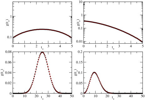
Figure 2: A comparison of a simulation and eq. (Statistics of trajectories in two-state master equations) for the function $g(t_{+}|T)$. The parameters are $T=5$ (top figures) and $T=50$ (bottom figures). The rates are $k_{+}=k_{-}=0.5$ (left figures) and $k_{-}=0.8$ and $k_{+}=0.2$ (right figures). Lines (red on-line) are the analytic curves; the black point are averages over $10^{7}$ simulations of the master equation. Notice the effect of the Delta functions (first and last point) in the top figures, where the probabilities are in log scale. (We do not plot the delta functions in the analytic curves).

In Fig. (2) we plot the function $g(t_{+}|T)$ for several values of the parameters, and we compare it with simulations of the master equations. In all cases studied, there is perfect agreement between the simulations and the present analytic result.

An interesting limit of eq. (Statistics of trajectories in two-state master equations) is that of large $T$. Using the asymptotic expression $\lim_{x\to\infty}\left[I_{\nu}(x)\right]={\rm exp}\left(x/\sqrt{2\pi z}\right)$, we see that the leading term in $1/T$ is

$$g(t_{+}|T)\approx\sqrt{\frac{2}{\pi z}}\frac{k_{+}k_{-}}{k_{T}}\,{\rm e}^{-\left(\sqrt{(k_{-}t_{+})}-\sqrt{k_{+}(T-t_{+})}\right)^{2}}\ ,$$ (10)

which has exponential tails expected from large deviation arguments touchette .

Another issue that can be addressed in this framework is the probability, $h(N)$, of observing precisely $N$ transitions in a time interval of $T$. This is simply:

$$h(N)=\int_{0}^{T}dt_{+}[P^{eq}_{-}\,\mathcal{P}(-,T,t_{+},N)+P^{eq}_{+}\mathcal{P}(+,T,t_{+},N)].$$ (11)

Using the above expressions for the various terms and performing the integral, we find two different expressions, one for $N$ odd:

$$h(N)=\frac{2\sqrt{\pi}(k_{+}k_{-})^{(N+1)/2}}{((N-1)/2)!k_{T}}\left(\frac{T}{k_{-}-k_{+}}\right)^{\frac{N}{2}}\times$$

$$\times{\rm e}^{-(k_{+}+k_{-})T/2}\,I_{N/2}\left(\zeta\right)$$ (12)

and one for $N$ even:

$$h(N)=\frac{\sqrt{\pi}T(k_{-}k_{+})^{(N/2)}}{2k_{T}(N/2)!}\,\left(\frac{T}{k_{-}-k_{+}}\right)^{\frac{(N-1)}{2}}\!\!\!{\rm e}^{-(k_{+}+k_{-})\frac{T}{2}}\times$$

$$\times\left[(k_{-}+k_{+})\,I_{(N-1)/2}\left(\zeta\right)+(k_{-}-k_{+})\,I_{(N+1)/2}\left(\zeta\right)\right]\qquad$$ (13)

with $\zeta=(k_{-}-k_{+})T/2$.

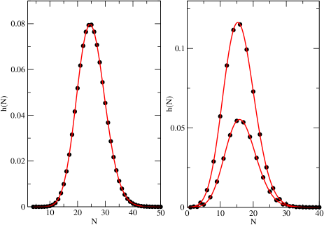
Figure 3: The probabilities, $h(N)$, of observing $N$ transitions in a time $T=50$. Transition rates are (left) $k_{+}=k_{-}=0.5$ (right) and $k_{+}=0.2$ and $k_{-}=0.8$ (left). The points represent statistics collected over $10^{7}$ simulations. The solid lines (red on-line) are the analytic results of eqns. (Statistics of trajectories in two-state master equations) and (Statistics of trajectories in two-state master equations). The left figure corresponds to the symmetric limit with $k+{+}=k_{-}=0.5$ in which both distributions collapse into a Poisson distribution. Notice the even-odd asymmetry in the right figure.

In evaluating the two expressions above, care must be taken to pick up the proper branch of the half-integer powers according to the requirement that the function $h(N)$ should be real and positive. In Fig. (3) we compare the distribution $h(N)$ with simulations of the master equation. Here, too, perfect agreement is found. The left panel shows a symmetric case with $k_{+}=k_{-}=0.5$ for which eqns. (Statistics of trajectories in two-state master equations) and (Statistics of trajectories in two-state master equations) each have as limit a Poisson distribution, $h(N)=\lambda^{N}{\rm e}^{-}{\lambda}/N!$ with $\lambda=T/k_{+}=T/k_{-}$. The right panel, for the case $k_{+}=0.2$ and $k_{-}=0.8$, is less trivial. The asymmetry in the rates is reflected in a difference between the distributions for $N$ even and $N$ odd. This corresponds to the physical fact that one of the states is short-lived and the other long-lived, so that is more likely to observe an even number of transitions. In the asymmetric case, accurate numerical studies indicate that the average number of transitions is $\bar{N}=T/\tilde{k}$ with $\tilde{k}=k_{+}k_{-}/[2(k_{+}+k_{-})]$.

In summary, we have shown that the probability distributions associated with the trajectories of master equations can be expressed in general as a product over single-state properties. This can be particularly useful for systems composed of a few states as demonstrated by the exact determination of several statistical quantities of two-state master equations for which results can be expressed simply in terms of modified Bessel functions. While the methods presented here can be applied to the evaluation of individual trajectories in more complex problems, summation over all trajectories becomes increasingly difficult as the number of states increases. If, however, almost all rates are small, the dynamics of the system can be dominated by a relatively small number of trajectories. For example, this is often the case in chemical kinetics, where average reaction paths may be well defined even for high-dimensional dynamics zuckermann . In such cases, our methods could provide a way to detect these dominant trajectories and to assess their probabilities.

- (1) M.B. Elowitz, A.J. Levine, E.D. Siggia, P.S. Swain, Science 297(5584) pp.1183-1186 (2002).
- (2) J. Lebowitz and H. Spohn, Jour. Stat. Phys. 95, pp 333-364 (1999).
- (3) M. Esposito, U. Harbola and S. Mukamel, Phys. Rev. E 76, 031132 (2007).
- (4) J. Harris and G. M. Schutz, J. Stat. Mech. P07020 (2007).
- (5) C. W. Gardiner, Handbook of stochastic methods (Springer, Berlin 1983).
- (6) D. T. Gillespie, J. Phys. Chem. 81, pp. 2340-2361 (1977).
- (7) S. Pigolotti and A. Vulpiani, Jour. Chem. Phys. 128(154114), (2008).
- (8) See, e.g.,C. Itzykson, J. M. Drouffe, Statistical Field Theory vol. 1, Cambridge University Press (1989).
- (9) L. Peliti, J. Phys. (Paris) 46, 1469 (1985).
- (10) J. Cardy, in The Mathematical Beauty of Physics, edited by J. Drouffe and J. B. Zuber (World Scientific, Singapore 1997)
- (11) G. Margolin and E. Barkai, Phys. Rev. Lett. 94, 080601 (2005).
- (12) F. Shikerman and E. Barkai, Phys. Rev. Lett. 99. 208302 (2007).
- (13) G. Bonnet, O. Krichevsky, and A. Libchaber, Proc. Natl. Acad. Sci. 95(15) pp. 8602-8606 (1998).
- (14) R. Zwanzig, Proc. Natl. Acad. Sci. 94(1), pp. 148-150 (1997).
- (15) F. Ritort, C. Bustamante, I. Tinoco, Proc. Natl. Acad. Sci. 99(21), pp. 13544-13548 (2002)
- (16) A. M. Berezhkovskii, A. Szabo and J. Weiss, Jour. Chem. Phys. 110(18) pp. 9145-9150 (1999).
- (17) H. Touchette, arXiv:0804.0327v1.
- (18) D. M. Zuckermann and T. B. Woolf, Jour. Chem. Phys 111(21), pp. 9475-9484 (1999).