Three-Point Correlations in f(R) Models of Gravity

Abstract

Modifications of general relativity provide an alternative explanation to dark energy for the observed acceleration of the universe. We calculate quasilinear effects in the growth of structure in $f(R)$ models of gravity using perturbation theory. We find significant deviations in the bispectrum that depend on cosmic time, length scale and triangle shape. However the deviations in the reduced bispectrum $Q$ for $f(R)$ models are at the percent level, much smaller than the deviations in the bispectrum itself. This implies that three-point correlations can be predicted to a good approximation simply by using the modified linear growth factor in the standard gravity formalism. Our results suggest that gravitational clustering in the weakly nonlinear regime is not fundamentally altered, at least for a class of gravity theories that are well described in the Newtonian regime by the parameters $G_{\rm eff}$ and $\Phi/\Psi$. This approximate universality was also seen in the N-body simulation measurements of the power spectrum by Stabenau & Jain (2006), and in other recent studies based on simulations. Thus predictions for such modified gravity models in the regime relevant to large-scale structure observations may be less daunting than expected on first principles. We discuss the many caveats that apply to such predictions.

I Introduction

The energy contents of the universe pose an interesting puzzle, in that general relativity (GR) plus the Standard Model of particle physics can only account for about $4\%$ of the energy density inferred from observations. By introducing dark matter and dark energy, which account for the remaining $96\%$ of the total energy budget of the universe, cosmologists have been able to account for a wide range of observations, from the overall expansion of the universe to the large scale structure of the early and late universe Reviews .

The dark matter/dark energy scenario assumes the validity of GR at galactic and cosmological scales and introduces exotic components of matter and energy to account for observations. Since GR has not been tested independently on these scales, a natural alternative is that GR itself needs to be modified on large scales. This possibility, that modifications in GR on galactic and cosmological scales can replace dark matter and/or dark energy, has become an area of active research in recent years.

Attempts have been made to modify GR with a focus on galactic MOND or cosmological scales DGP ; fR ; Sahni2005 . Modified Newtonian Dynamics (MOND) and its relativistic version (Tensor-Vector-Scalar, TeVeS)  MOND attempt to explain observed galaxy rotation curves without dark matter (but have problems on larger scales). The DGP model DGP , in which gravity lives in a 5D brane world, naturally leads to late time acceleration of the universe.

Adding a correction term $f(R)$ to the Einstein-Hilbert action fR also allows late time acceleration of the universe to be realized.

In this paper we will focus on modified gravity (MG) theories that are designed as an alternative to dark energy to produce the present day acceleration of the universe. In these models, such as DGP and $f(R)$ models, gravity at late cosmic times and on large-scales departs from the predictions of GR. By design, successful MG models are difficult to distinguishable from viable DE models against observations of the expansion history of the universe. However, in general they predict a different growth of perturbations which can be tested using observations of large-scale structure (LSS) Yukawa ; Stabenau2006 ; Skordis06 ; Dodelson06 ; DGPLSS ; consistencycheck ; Koyama06 ; fRLSS ; Zhang06 ; Bean06 ; MMG ; Uzan06 ; Caldwell07 ; Amendola07 ; HuSaw3 .

In this paper we consider the quasilinear regime of clustering in which perturbation theory calculations are valid. We explore what $f(R)$ modifications to gravity predict about the behavior of the three-point correlation function. In §II we outline the particular type of $f(R)$ gravity model we will be using for our calculations. In §III we introduce the fundamentals of perturbation theory and in particular how it applies to modified gravity. In §IV we focus on second order corrections and in particular the Bispectrum. In §V we present our results and compare with other studies of the nonlinear regime. In §VI we discuss the implications for observations.

II The $f(R)$ modified gravity model

In general $f(R)$ models are a modification of the Einstein-Hilbert action of the form:

$$S=\int d^{4}x\sqrt{-g}\left[\frac{R+f(R)}{2\kappa^{2}}+{\cal L}_{m}\right],$$ (1)

where $R$ is the curvature, $\kappa^{2}=8\pi G$, and ${\cal L}_{m}$ is the matter Lagrangian. A major issue with gravity modifications has been that while they are successful at explaining the acceleration of the universe, they also tend to fail to comply with Solar system (very small scales) observations. Recently, though, the so called Chameleon mechanism was found Khoury1 that makes it possible to overcome this problem. Significant attempts have been made to include Chameleon behavior KhouryDGP in DGP theories as well. One example of an $f(R)$ model that exhibits Chameleon behavior was constructed by Hu and Sawicki HuSaw . The functional form of $f(R)$ there is derived from a list of observational requirements: it should mimic $\Lambda CDM$ in the high-redshift regime as well as produce $\Lambda CDM$ acceleration of the universe at low redshift without a true cosmological constant; it should also fit Solar system observations.

The particular form chosen by HuSaw is:

$$f(R)=-m^{2}\frac{c_{1}(R/m^{2})^{n}}{c_{2}(R/m^{2})^{n}+1}$$ (2)

with

$$m^{2}\equiv\frac{\kappa^{2}\bar{\rho}_{0}}{3}=(8315Mpc)^{-2}\left(\frac{\Omega_{m}h^{2}}{0.13}\right)$$ (3)

where $\kappa\equiv 8\pi G$ and $\bar{\rho}_{0}$ is the average density today. In this model, modifications to GR only appear at low redshift, when we are safely in the matter dominated regime. The properties of the model are well described by the auxiliary scalar field $f_{R}\equiv\frac{df(R)}{dR}$.

Before going to the expansion history, it is worth briefly reviewing the main features of this model, following the original presentation in HuSaw . The trace of the modified Einstein equations serves as the equation of motion for $f_{R}$:

$$3\Box f_{R}-R+f_{R}R-2f=-\kappa^{2}\rho,$$ (4)

or, in terms of the effective potential,

$$\Box f_{R}=\frac{\partial V_{\rm eff}}{\partial f_{R}}.$$ (5)

The effective mass for the $f_{R}$ field is then given by the second derivative of $V_{\rm eff}$, evaluated at its extremum:

$$m^{2}_{\rm eff}=\frac{\partial^{2}V_{\rm eff}}{\partial f^{2}_{R}}=\frac{1}{3}\left(\frac{1+f_{R}}{f_{RR}}-R\right).$$ (6)

The Compton wavelength of the field is then given by $\lambda_{f_{R}}\equiv m^{-1}_{\rm eff}$.

It is very convenient to introduce a dimensionless quantity:

$$B=\frac{f_{RR}}{1+f_{R}}R^{{}^{\prime}}\frac{H}{H^{{}^{\prime}}}$$ (7)

It has been shown HuSaw that in the high-curvature regime $B$ is connected to the Compton wavelength via:

$$B^{1/2}\sim\lambda_{f_{R}}H$$ (8)

and thus is essentially the Compton wavelength of $f_{R}$ at the background curvature in units of the horizon length.

In the static limit with $|f_{R}|\ll 1$ and $|f/R|\ll 1$, Eqn. 4 becomes

$$\bigtriangledown^{2}f_{R}\approx\frac{1}{3}(R-\kappa^{2}\rho)$$ (9)

where $\rho$ is the local density. This equation has 2 modes of solutions. One is the very high curvature $R\approx\kappa^{2}\rho$ and the other one is the low curvature (but still high compared to the background density) $R\ll\kappa^{2}\rho$. For more on the interplay of these two regimes and applications in solar system observations see HuSaw .

Let’s now move on to the expansion history. For the model to yield behavior that is observationally viable requires a choice for the present day value of the $f_{R}$ field $f_{R0}\ll 1$. This is equivalent to $R_{0}\gg m^{2}$. In that case the approximation $R\gg m^{2}$ is valid for the whole expansion history and we have:

$$\lim_{m^{2}/R\rightarrow 0}f(R)\approx-\frac{c_{1}}{c_{2}}m^{2}+\frac{c_{1}}{c^{2}_{2}}m^{2}\left(\frac{m^{2}}{R}\right)^{n}$$ (10)

In the limiting case of $c_{1}/c^{2}_{2}\rightarrow 0$ at fixed $c_{1}/c_{2}$ we obtain a cosmological constant behavior $\Lambda CDM$. Thus to approximate the $\Lambda CDM$ expansion history with a cosmological constant $\Omega_{\Lambda}$ and matter density $\Omega_{m}$ we set:

$$\frac{c_{1}}{c_{2}}\approx 6\frac{\Omega_{\Lambda}}{\Omega_{m}}$$ (11)

This leaves 2 remaining parameters to play with: $n$ and $c_{1}/c^{2}_{2}$ to control how closely the model mimics $\Lambda CDM$. Larger n mimics until later in the expansion history, while smaller $c_{1}/c^{2}_{2}$ mimics it more closely.

For flat $\Lambda CDM$ we have the following relations:

$$R\approx 3m^{2}\left(a^{-3}+4\frac{\Omega_{\Lambda}}{\Omega_{m}}\right)$$ (12)

$$f_{R}=-n\frac{c_{1}}{c^{2}_{2}}\left(\frac{m^{2}}{R}\right)^{n+1}$$ (13)

As we will see later these are the necessary ingredients for the application of perturbation theory to the model.

Finally we need to obtain a suitable parametrization of the mode. At the present epoch we have:

$$R_{0}\approx m^{2}\left(\frac{12}{\Omega_{m}}-9\right)$$ (14)

$$f_{R0}\approx-n\frac{c_{1}}{c^{2}_{2}}\left(\frac{12}{\Omega_{m}}-9\right)^{-n-1}$$ (15)

In particular, for $\Omega_{\Lambda}=0.76$ and $\Omega_{m}=0.24$, we have $R_{0}=41m^{2}$ and $f_{R0}\approx-n\ c_{1}/c^{2}_{2}/(41)^{n+1}$. ¿From now on we will parametrize the model through $f_{R0}$ and $n$. Fig. 9 in HuSaw shows that there is a wide range of viable parameter values which satisfy Solar system and Galaxy requirements. We re-iterate that what makes this particular $f(R)$ model viable is its Chameleon behavior – the possibility of uniting galaxy and solar system observations with the expansion of the Universe.

III Perturbation Formalism

By definition, the dark sector (dark matter and dark energy) can only be inferred from its gravitational consequences. In general relativity, gravity is determined by the total stress-energy tensor of all matter and energy ($G_{\mu\nu}=8\pi G\ T_{\mu\nu}$).

We may consider the Hubble parameter $H(z)$ to be fixed by observations. In a dark energy model, $\bar{\rho}$ is given by the Friedman equation of GR: $\bar{\rho}=3H^{2}/8\pi G$. The equation of state parameter is $w=-1-2\dot{H}/3H^{2}$. The corresponding modified gravity model has matter density to be determined from its Friedman-like equation. We will consider MG models dominated by dark matter and baryons at late times.

III.1 Metric and fluid perturbations

With the smooth variables fixed, we will consider perturbations as a way of testing the models. In the Newtonian gauge, scalar perturbations to the metric are fully specified by two scalar potentials $\Psi$ and $\Phi$:

$$ds^{2}=-(1-2\Psi)\ dt^{2}+(1-2\Phi)\ a^{2}(t)\ d{\vec{x}}^{2}$$ (16)

where $a(t)$ is the expansion scale factor. This form for the perturbed metric is fully general for any metric theory of gravity, aside from having excluded vector and tensor perturbations (see Bertschinger2006 and references therein for justifications). Note that $\Psi$ corresponds to the Newtonian potential for the acceleration of particles, and that in general relativity $\Phi=-\Psi$ in the absence of anisotropic stresses.

A metric theory of gravity relates the two potentials above to the perturbed energy-momentum tensor. We introduce variables to characterize the density and velocity perturbations for a fluid, which we will use to describe matter and dark energy. The density fluctuation $\delta$ is given by

$$\delta({\vec{x}},t)\equiv\frac{\rho({\vec{x}},t)-{\bar{\rho}(t)}}{\bar{\rho}(t)}$$ (17)

where $\rho({\vec{x}},t)$ is the density and ${\bar{\rho}(t)}$ is the cosmic mean density. The second fluid variable is the divergence of the peculiar velocity

$$\theta\equiv\nabla_{j}T_{0}^{j}/(\bar{p}+\bar{\rho})={\vec{\nabla}}\cdot{\vec{v}},$$ (18)

where $\vec{v}$ is the (proper) peculiar velocity. Choosing $\theta$ instead of the vector ${\bf v}$ implies that we have assumed ${\bf v}$ to be irrotational. Our notation and formalism follows that of JZ .

In principle, observations of large-scale structure can directly measure the four perturbed variables introduced above: the two scalar potentials $\Psi$ and $\Phi$, and the density and velocity perturbations specified by $\delta$ and $\theta$. It is convenient to work with the Fourier transforms, such as:

$$\hat{\delta}(\vec{k},t)=\int d^{3}x\ \delta(\vec{x},t)\ e^{-i{\vec{k}}\cdot{\vec{x}}}$$ (19)

When we refer to length scale $\lambda$, it corresponds to a a statistic such as the power spectrum on wavenumber $k=2\pi/\lambda$. We will henceforth work exclusively with the Fourier space quantities and drop the $\hat{}$ symbol for convenience.

III.2 Linearized fluid equations

We will use the perturbation theory equations for the quasi-static regime of the growth of perturbations. We begin with the fluid equations in the Newtonian gauge, following the formalism and notation of Ma95 .

For minimally coupled gravity models with baryons and cold dark matter, but without dark energy, we can neglect pressure and anisotropic stress terms in the evolution equations to get the continuity equation:

$$\dot{\delta}=-\left(\frac{\theta}{a}-3\dot{\Phi}\right)\simeq-\frac{\theta}{a}\ ,$$ (20)

where the second equality follows from the quasi-static approximation as for GR. The Euler equation is:

$$\dot{\theta}=-H\theta-\frac{k^{2}\Psi}{a}\ .$$ (21)

We parametrize modifications in gravity by two functions $\tilde{G}_{\rm eff}(k,t)$ and $\eta(k,t)$ to get the analog of the Poisson equation and a second equation connecting $\Phi$ and $\Psi$ Zhang7 ; JZ . We first write the generalization of the Poisson equation in terms of an effective gravitational constant $G_{\rm eff}$:

$$k^{2}\Phi=-4\pi G_{\rm eff}(k,t)\bar{\rho}_{\rm MG}a^{2}\delta_{\rm MG}\ .$$ (22)

Note that the potential $\Phi$ in the Poisson equation comes from the spatial part of the metric, whereas it is the “Newtonian” potential $\Psi$ that appears in the Euler equation (it is called the Newtonian potential as its gradient gives the acceleration of material particles). Thus in MG, one cannot directly use the Poisson equation to eliminate the potential in the Euler equation. A more useful version of the Poisson equation would relate the sum of the potentials, which determine lensing, with the mass density. We therefore introduce $\tilde{G}_{\rm eff}$ and write the constraint equations for MG as

$$k^{2}(\Phi-\Psi)=-8\pi\tilde{G}_{\rm eff}(k,t)\bar{\rho}_{\rm MG}a^{2}\delta_{\rm MG}$$ (23)

$$\Phi=-\Psi\ \eta(k,t)$$ (24)

where $\tilde{G}_{\rm eff}=G_{\rm eff}(1+\eta^{-1})/2$.

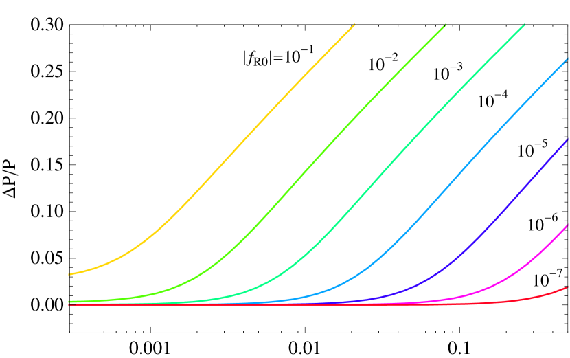
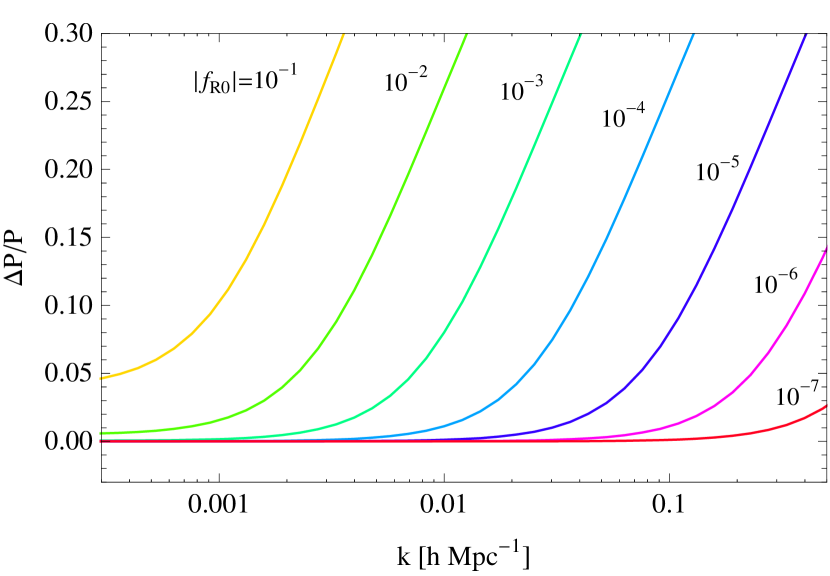
Figure 1: Fractional change at $z=0$ in the density power spectrum of the $f(R)$ model compared to $\Lambda CDM$ for a set of choices of $f_{R0}$. The upper panel is the $n=4$ model, while the lower panel has $n=1$. This figure can be compared with Fig. 4 in HuSaw .

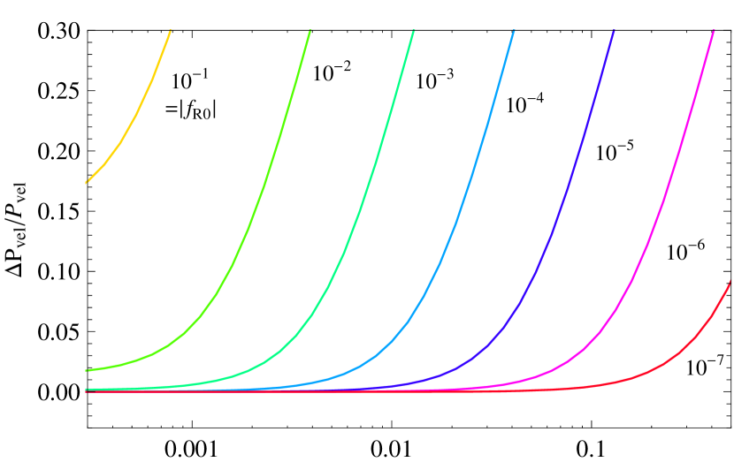
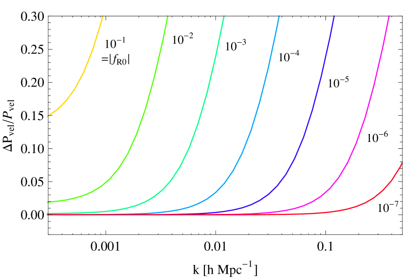
Figure 2: Fractional change at $z=0$ in the velocity power spectrum of the $f(R)$ model compared to $\Lambda CDM$ for a set of choices of $f_{R0}$. The upper panel is the $n=4$ model, while the lower panel has $n=1$.

The parameter $\tilde{G}_{\rm eff}$ characterizes deviations in the ($\Phi-\Psi$)-$\delta$ relation from that in GR. Since the combination $\Phi-\Psi$ is directly responsible for gravitational lensing, $\tilde{G}_{\rm eff}$ has a specific physical meaning: it determines the power of matter inhomogeneities to distort light. This is the reason we prefer it over working with more direct generalization of Newton’s constant, ${G}_{\rm eff}$.

With the linearized equations above, the evolution of either the density or velocity perturbations can be described by a single second order differential equation. From Eqns. 20 and 21 we get, for the linear solution, $\delta(\vec{k},t)\simeq\delta_{initial}(\vec{k})D(k,t)$,

$$\ddot{\delta}+2H\dot{\delta}+\frac{k^{2}\Psi}{a}=0.$$ (25)

For a given theory, Eqns. 23 and 24 then allow us to substitute for $\Psi$ in terms of $\delta$ to determine $D(k,t)$, the linear growth factor for the density:

$$\ddot{D}+2H\dot{D}-\frac{8\pi\tilde{G}_{\rm eff}}{(1+\eta)}\bar{\rho}a^{2}\ D=0.$$ (26)

What we need now are $\tilde{G}_{\rm eff}$ and $\eta$ for our modified gravity model.

III.3 Parametrized post-Friedmann framework

Hu & Sawicki HuSaw also developed a formalism for simultaneous treatment of the super-horizon and quasi-static regime for modified gravity theories (in particular $f(R)$ and DGP) HuSaw2 . They begin by describing the different regimes individually and the requirements they impose on the structure of such models. Consequently they describe a linear theory parametrization of the super-horizon and the quasi-static regime and test it against explicit calculation. What is important for this paper is the proposed interpolation function for the metric ratio

$$g=\frac{\Phi+\Psi}{\Phi-\Psi}$$ (27)

For consistency we will express formulae from Hu & Sawicki in terms of physical time instead of expansion factor. We start with a background FRW universe for which we have the curvature in terms of the Hubble parameter $R=6\dot{H}+12H^{2}$. As we mentioned the background evolution $H$ is chosen to match that of flat $\Lambda CDM$. We can then compute the Compton parameter $B$ for our preferred model since we know what $f(R)$, $R$ and $H$ are:

$$B=\frac{f_{RR}}{1+f_{R}}\dot{R}\frac{H}{\dot{H}}$$ (28)

The next step is to look at the super-horizon regime. In that case we know how to calculate the potentials $\Phi$ and $\Psi$. Their evolution is given by HuSaw3 :

$$\begin{gathered}\ddot{\Phi}+\left(1-\frac{\ddot{H}}{H\dot{H}}+\frac{\dot{B}}{H(1-B)}+B\frac{\dot{H}}{H^{2}}\right)H\dot{\Phi}+\\ \left(2\frac{\dot{H}}{H^{2}}-\frac{\ddot{H}}{H\dot{H}}+\frac{\dot{B}}{H(1-B)}\right)H^{2}\Phi=0,(k_{H}\rightarrow 0)\end{gathered}$$ (29)

$$\Psi=\frac{-\Phi-B\dot{\Phi}/H}{1-B},(k_{H}\rightarrow 0)$$ (30)

This allows us to compute $g_{SH}=g(t,k_{H}\rightarrow 0)$.

Furthermore in the case of subhorizon evolution where $k_{H}=k/a(t)H\gg 1$ we have $g_{QS}=-\frac{1}{3}$ HuSaw3 .

According to HuSaw2 in the case of $f(R)$ theories we can use the following interpolation functions for the metric ratio:

$$g(t,k)=\frac{g_{SH}+g_{QS}(c_{g}k_{H})^{n_{g}}}{1+(c_{g}k_{H})^{n_{g}}}$$ (31)

The evolution then is well described by HuSaw2 $c_{g}=0.71B^{1/2}$ and $n_{g}=2$ In terms of the post-Newtonian parameter: $\eta=-\Phi/\Psi$ we have $g=(\eta-1)/(\eta+1)$.

We still need one more ingredient, $\tilde{G}_{\rm eff}$, which is given by HuSaw2

$$\tilde{G}_{\rm eff}(k,t)=\frac{G}{1+f_{R}}$$ (32)

We now have all the needed components to use in equation (26) for the growth factor of density perturbations. Calculations of the fractional change in the linear density power spectrum compared to GR have been done HuSaw . We show these in Fig. 1, using $\tilde{G}_{\rm eff}$ and $\eta$ for the particular model we investigate. We have assumed the transfer function for the concordance $\Lambda-$CDM model consistent with the 5-year WMAP data Dunkley et al. (2008).

We can also use the relations given above to obtain the linear growth factors for $\theta$ and the potentials from $D$. Note that in general the growth factors for the potentials have a different $k$ dependence than $D$.

IV The Bispectrum in Perturbation Theory

IV.1 Nonlinear Fluid Equations

The fluid equations in the Newtonian regime are given by the continuity, Euler and Poisson equations. Keeping the nonlinear terms that have been discarded in the study of linear perturbations above, the continuity equations gives:

$$\dot{\delta}+\theta=-\int\frac{d^{3}k_{1}}{(2\pi)^{3}}\frac{{\vec{k}}\cdot{\vec{k}_{1}}}{k_{1}^{2}}\theta(\vec{k_{1}})\delta({\vec{k}}-{\vec{k}_{1}})$$ (33)

where the term on the right shows the nonlinear coupling of modes. Note that the time derivatives are with respect to conformal time in this section.

The Euler equation is

$$\dot{\theta}+H\theta+k^{2}\Psi=-\int\frac{d^{3}k_{1}}{(2\pi)^{3}}\frac{k^{2}{\vec{k}_{1}}\cdot(\vec{k}-\vec{k}_{1})}{2k_{1}^{2}|{\vec{k}_{1}}-{\vec{k}_{2}}|^{2}}\theta(\vec{k_{1}})\theta({\vec{k}}-{\vec{k}_{1}})$$ (34)

We neglect pressure and anisotropic stress as the energy density is taken to be dominated by non-relativistic matter Jain1994 . The Poisson equation is given by Eqn. 23 and supplemented by the relation between $\Psi$ and $\Phi$ given by Eqn. 24. Using these equations we can substitute for $\Psi$ in the Euler equation to get

$$\dot{\theta} + H\theta+\frac{8\pi\tilde{G}_{\rm eff}}{(1+\eta)}\bar{\rho}_{\rm MG}a^{2}\delta$$ (35)

$$= \,-\int\frac{d^{3}k_{1}}{(2\pi)^{3}}\frac{k^{2}{\vec{k}_{1}}\cdot({\vec{k}-\vec{k}_{1}})}{2k_{1}^{2}|{\vec{k}_{1}}-{\vec{k}_{2}}|^{2}}\theta(\vec{k_{1}})\theta({\vec{k}}-{\vec{k}_{1}})$$

Eqns. 33 and 35 are two equations for the two variables $\delta$ and $\theta$. They constitute a fully nonlinear description and can be solved once $\eta$ and $\tilde{G}_{\rm eff}$ are specified. An important caveat is that they may nevertheless be invalid on strongly nonlinear scales or for particular MG theories. For the $f(R)$ model considered here, they are valid on scales well above 1 Mpc; on smaller scales the chameleon mechanism modifies the growth of structure LimaHu . Since we will use perturbation theory, our approach breaks down once $\delta\sim 1$ in any case.

Next we consider perturbative expansions for the density field and the resulting behavior of the power spectrum and bispectrum. Let $\delta=\delta_{1}+\delta_{2}+...$ where $\delta_{2}\sim O(\delta_{1}^{2})$. In the quasilinear regime, i.e. on length scales between $\sim$10-100 Mpc, mode coupling effects can be calculated using perturbation theory. While this is strictly true only for general relativity, a MG theory that is close enough to GR to fit observations can also be expected to have this feature.

For MG, following JZ , let us simplify the notation by introducing the function:

$$\zeta(k,t)=\frac{8\pi\tilde{G}_{\rm eff}}{(1+\eta)},$$ (36)

which is simply $4\pi G$ in GR but can vary with time and scale in MG theories. The evolution of the linear growth factor is given by substituting for $\Psi$ in Eqn. 37 to get (as above, but with conformal time here)

$$\ddot{\delta_{1}}+H\dot{\delta_{1}}-\zeta\bar{\rho}a^{2}\delta_{1}=0.$$ (37)

The linear growth factor has a scale dependence for our $f(R)$ as shown in Fig. 1.

In addition we show below that the second order solution has a functional dependence on $\tilde{G}_{\rm eff}$ and $\eta$ that can differ from GR. Thus potentially distinct signatures of the scale and time dependence of $\tilde{G}_{\rm eff}(k,z)$ can be inferred from higher order terms. These rely either on features in $k$ and $t$ in measurements of $P_{\Phi-\Psi}$ and $P_{\delta}$, or on the three-point functions which can have distinct signatures of MG even at a single redshift Bernardeau2004 . Quasilinear signatures due to $\eta(k,z)$ can also be detected via second order terms in the redshift distortion relations for the power spectrum and bispectrum. Our discussion generalizes that of Yukawa who examined a Yukawa-like modification of the Newtonian potential.

IV.2 Second order solution

From a perturbative treatment of Eqns. 33 and 35 the second order term for the growth of the density field is given by JZ

$$\ddot{\delta_{2}}+H\dot{\delta_{2}}-\bar{\rho}a^{2}\zeta\delta_{2}=$$

$$HI_{1}[\dot{\delta_{1}},\delta_{1}]+I_{2}[\dot{\delta_{1}},\dot{\delta_{1}}]+\dot{I_{1}}[\dot{\delta_{1}},\delta_{1}],$$ (38)

where $I_{1}$ and $I_{2}$ denote convolution like integrals of the two arguments shown, given by the right-hand side of equations 33 and 35 as follows

$$I_{1}[\dot{\delta_{1}},\delta_{1}](\vec{k})=\int\frac{d^{3}k_{1}}{(2\pi)^{3}}\frac{{\vec{k}}\cdot{\vec{k}_{1}}}{k_{1}^{2}}\dot{\delta_{1}}(\vec{k_{1}})\delta_{1}({\vec{k}}-{\vec{k}_{1}})$$ (39)

and

$$I_{2}[\dot{\delta_{1}},\dot{\delta_{1}}](\vec{k})=\int\frac{d^{3}k_{1}}{(2\pi)^{3}}\frac{k^{2}{\vec{k}_{1}}\cdot(\vec{k}-\vec{k}_{1})}{2k_{1}^{2}|{\vec{k}_{1}}-{\vec{k}_{2}}|^{2}}\dot{\delta_{1}}(\vec{k_{1}})\dot{\delta_{1}}({\vec{k}}-{\vec{k}_{1}}).$$ (40)

Finally, the last term in Eqn. 38 is simply $\dot{I_{1}}[\dot{\delta_{1}},\delta_{1}]=I_{1}[\ddot{\delta_{1}},\delta_{1}]+I_{1}[\dot{\delta_{1}},\dot{\delta_{1}}]$. Note that by continuing the iteration, higher order solutions can be obtained.

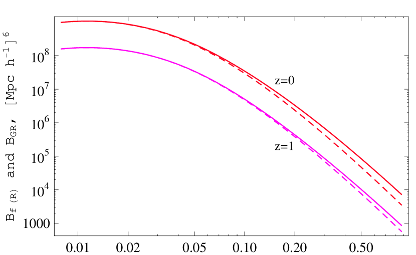
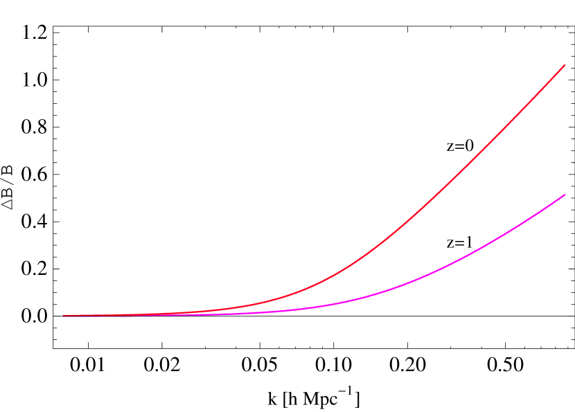
Figure 3: Upper panel: The Bispectrum of the $f(R)$ model for equilateral triangles depending on scale for the $f(R)$ model with $f_{R0}=10^{-5}$, $n=1$. The corresponding regular gravity bispectrum is shown as the dashed curve. Lower panel: The Ratio of the f(R) Bispectrum to the regular gravity one.

IV.3 Three-point correlations

Distinct quasilinear effects are found in three-point correlations – we will use the Fourier space bispectrum. Recently Tatekawa & Tsujikawa have performed a similar perturbative analysis and presented results on the skewness TatekawaTsujikawa . We prefer to use the bispectrum as it allows one to study specific quasilinear signatures contained in the configuration dependence of triangle shapes. The bispectrum for the density field $B_{\delta}$ is defined by

$$\langle\delta({\vec{k}_{1}})\delta({\vec{k}_{2}})\delta({\vec{k}_{3}})\rangle=(2\pi)^{3}\delta_{\rm D}({\vec{k}_{1}+\vec{k}_{2}+\vec{k}_{3}})B_{\delta}(\vec{k}_{1},\vec{k}_{2},\vec{k}_{3})$$ (41)

Since $B_{\delta}\sim\langle\delta^{3}\rangle\sim\langle\delta_{1}^{2}\delta_{2}\rangle$ (using $\langle\delta_{1}^{3}\rangle=0$ for an initially Gaussian density field) at tree level, the second order solution enters at leading order in the bispectrum. Note also that the wavevector arguments of the bispectrum form a triangle due to the Dirac delta function on the right-hand side above.

The bispectrum is the lowest order probe of gravitationally induced non-Gaussianity. A useful version of it is the reduced bispectrum $Q$, which for the density field $\delta$ is given by

$$Q_{\delta}\equiv\frac{B_{\delta}(\vec{k}_{1},\vec{k}_{2},\vec{k}_{3})}{P_{\delta}(k_{1})P_{\delta}(k_{2})+P_{\delta}(k_{2})P_{\delta}(k_{3})+P_{\delta}(k_{1})P_{\delta}(k_{3})}.$$ (42)

$Q$ is useful because it is insensitive to the amplitude of the power spectrum; thus e.g. at tree level and in the case of a scale free linear power spectrum $P(k)\sim k^{n}$ it is static and scale independent for regular gravityBernardeau2002 .

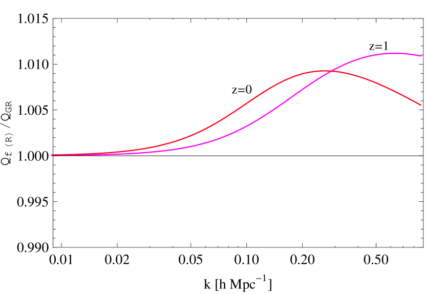
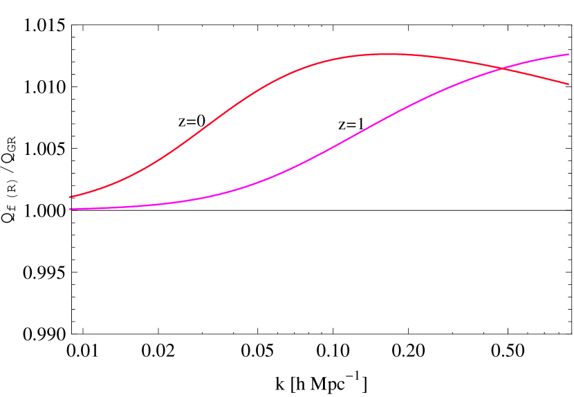
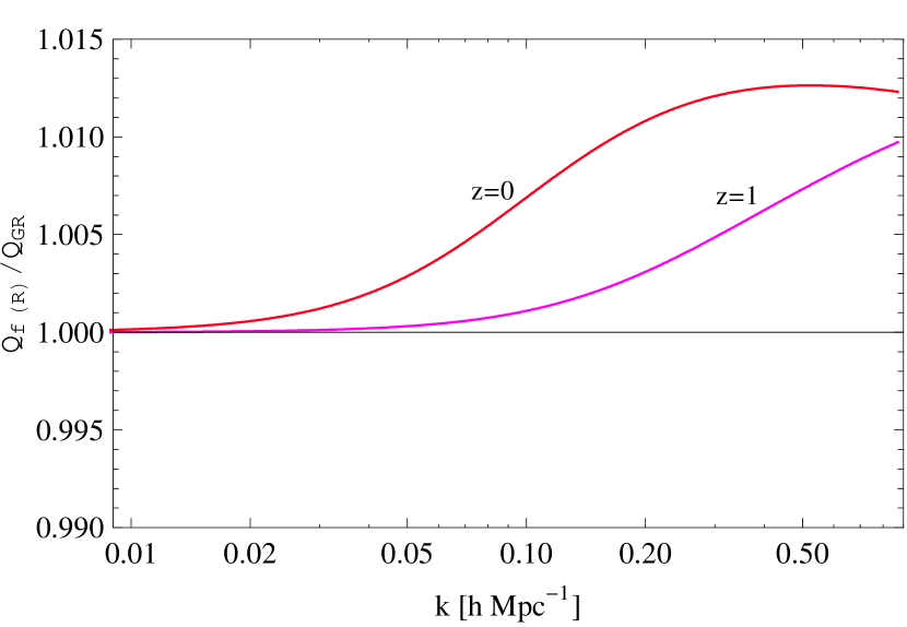
Figure 4: The reduced bispectrum $Q$ for equilateral triangles for the $f(R)$ model compared to regular gravity. Top panel: $f_{R0}=10^{-5}$, $n=1$. Middle panel: $f_{R0}=10^{-4}$, $n=4$. Bottom panel: $f_{R0}=10^{-5}$, $n=4$.

V Results

In Fig. 3 we present the bispectrum for the $f(R)$ model and its dependence on scale for two different redshifts. For comparison we also show the bispectra predicted in GR. In the lower panel we present the ratio of the $f(R)$ bispectra to that in GR. We have assumed the transfer function for the concordance $\Lambda-$CDM model consistent with the 5-year WMAP data Dunkley et al. (2008). Calculation is done at tree level with $\Omega_{m}=0.24$. The bispectra in $f(R)$ gravity are enhanced relative to GR, increasingly so at high-$k$. The enhancement is of order 10-20% for observationally relevant scales around $k\sim 0.1$ and redshifts below unity.

We turn our attention to the reduced bispectrum $Q$, which is expected to show features not associated with the linear power spectrum Bernardeau2002 . We show two relevant cases. The first one is with equilateral triangles, shown in Fig. 4. Deviations from GR are at the percent-level, which makes them impossible to detect with current measurements. Qualitatively, the parameters of the model do influence the scale and time dependence of the reduced bispectrum.

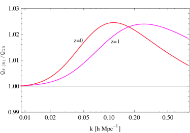
Figure 5: The reduced bispectrum $Q$ for isosceles triangles (ratio of sides lengths 1:3:3), where the x-axis shows the length of the smallest $k$ in the triangle. The ratio of $Q$ for the $f(R)$ model with $f_{R0}=10^{-5}$, $n=1$ to regular gravity is shown.

Slightly stronger deviations from regular gravity are observed for isosceles triangle configurations, shown in Fig. 5. Once again strong scale and time variation is observed when changing the model parameters. We also show the angular dependence of the reduced bispectrum for 3:1 ratio configurations and its comparison to regular gravity in Fig. 6.

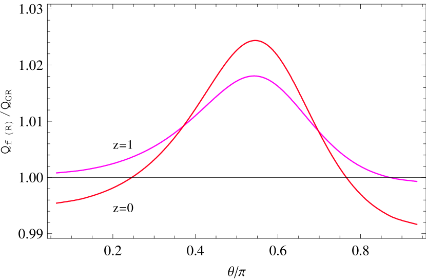
Figure 6: Upper panel: The angular dependence of the reduced bispectrum $Q$ for triangles with the two fixed side lengths in the ratio 1:3 and $k=0.1h$/Mpc for the smaller one. The $f(R)$ model with $f_{R0}=10^{-5}$, $n=1$ at $z=0$ is used. The dashed line shows the prediction for GR. Lower panel: Comparison to regular gravity at two redshifts. We can observe that for obtuse shapes ($\theta\sim 0$) our model predicts a lower $Q$ for $f(R)$ gravity, while for shapes close to isosceles it is enhanced.

V.1 Does the Linear Growth Factor Determine Nonlinear Clustering?

Quasilinear effects, and the bispectrum in particular, show signatures of gravitational clustering. However, we find that the reduced bispectrum $Q$ remains very close to to that of $GR$ in the modified gravity models we have considered (see also TatekawaTsujikawa for a related study). This is qualitatively similar to previous findings about the insensitivity of $Q$ to cosmological parameters within a GR context Bernardeau2002 .

Thus the deviations in the bispectrum are largely determined by the linear growth factor. Ambitious future surveys will be needed to achieve the percent level measurements required to probe the unique signatures of modified gravity in the bispectrum. On the other hand, this means that the bispectrum can be used as a consistency check on the power spectrum. It has been shown that the bispectrum contains information comparable to the power spectrum, thus improving the signal-to-noise Sefusatti et al. (2006) . Equally importantly, it is affected by sources of systematic error in different ways and contains signatures of gravitational clustering that are unlikely to be mimicked by other effects.

Currently the results of N-body simulations for this f(R) model LimaHu show that our assumptions are consistent with their result for the power spectrum in the regime of validity of perturbation theory (e.g. for $k\lesssim 0.3[h/Mpc]$). On smaller scales, the chameleon mechanism modifies the power spectrum.

Modifications to the Newtonian potential were simulated by Stabenau2006 (also see Yukawa ,Laszlo ). These simulation studies found that, to a good approximation, the nonlinear power spectra depend only on the initial conditions and linear growth. The standard fitting formulae for Newtonian gravity Smith2002 were adapted to predict the nonlinear spectrum at a given redshift. Therefore tests for modified gravity using the power spectrum require either a measurement of the scale dependent growth factor (in combination with the initial spectrum measured from the CMB), or of measurements at multiple epochs. More likely a combination of probes will be used for robust tests of gravity (see e.g. JZ ).

Related studies of nonlinear clustering in $f(R)$ models or DGP gravity are in progress Schmidt ; Martino ; Scoccimarro08 ; these authors are considering the power spectra, bispectra as well as halo properties, in particular the halo mass function. The $f(R)$ studies of LimaHu and Schmidt show distinct effects of the chameleon field on small scales (comparable to galaxy and cluster sized halos for most models); HuSaw2 suggest a fit for the nonlinear power spectrum with additional parameters that describe the transition to the small-scale regime. The DGP study of Scoccimarro08 requires inclusion of nonlinear terms in the Poisson equation. So clearly for different models there can be new nonlinearities and couplings to additional fields that impact the small-scale regime of clustering. Even so, for a class of models that includes the $f(R)$ models studied here, the quasistatic, Newtonian description parameterized by $\tilde{G}_{\rm eff}$ and $\eta=\Phi/\Psi$ applies over a wide range of scales relevant for large-scale structure observations. In this regime, to a good approximation, many clustering statistics can be predicted using the linear growth factor and the standard gravity formalism.

V.2 Implications for Lensing and Dynamics

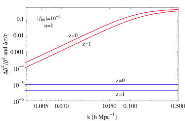
Figure 7: The fractional change in $\tau$ (blue lines) and $\beta^{2}$ (red lines) for the $f(R)$ model with $f_{R0}=10^{-5}$, $n=1$ compared to GR as a function of scale.

Lensing observations provide estimates of the convergence power spectrum and bispectrum (see e.g. Takada2004 ). For a rough estimate of these quantities, we take the source galaxies distribution to be a delta function at a given redshift and take the lensing matter to be situated at half the distance. Since we have taken the expansion history to be $\Lambda CDM$, so comoving distances are the same as in GR. With these approximations, $P_{\kappa}\propto P_{\Phi-\Psi}$. From Eqn. 23 we can see that the difference of the lensing behavior of our modified gravity case and the regular gravity one is given by (see also Bernardeau2004 )

$$P_{\Phi-\Psi}\propto P_{\delta}\left(\frac{\tilde{G}_{\rm eff}(k,t_{1/2})}{G}\right)^{2}$$ (43)

where $t_{1/2}$ is the physical time at the redshift of the lensing matter.

Thus we can write:

$$\frac{P_{\kappa MG}}{P_{\kappa GR}}\propto\frac{P_{\delta MG}}{P_{\delta GR}}\left(\frac{\tilde{G}_{\rm eff}(k,t_{1/2})}{G}\right)^{2}$$ (44)

Analogously we can see that the ratio of convergence bispectra behaves like $(\tilde{G}_{\rm eff}(k,t_{1/2})/G)^{3}$ but the ratio of the reduced bispectra behaves like

$$\frac{Q_{\kappa MG}}{Q_{\kappa GR}}\propto\frac{Q_{\delta MG}}{Q_{\delta GR}}\frac{G}{\tilde{G}_{\rm eff}(k,t_{1/2})}$$ (45)

Thus the convergence power spectrum and reduced bispectrum could be successfully used to differentiate and/or rule out models of modified gravity. Unfortunately in the currently discussed model we have Eqn. 32:

$$\tau(k,t(a))=\frac{\tilde{G}_{\rm eff}}{G}=\frac{1}{1+f_{R}(a)}$$ (46)

which deviates from unity at the order of $f_{R0}$, which is much smaller than unity. Thus the convergence power spectrum and reduced bispectrum follow almost identically the predictions for their matter counterparts. This means that the comparison of lensing to tracers of mass fluctuations does not reveal distinct signatures of $f(R)$ gravity.

The Newtonian potential $\Psi$ drives dynamical observables such as the redshift space power spectrum of galaxies JZ , Zhang7 . The velocity growth factor $D_{\theta}$ is related to the density growth factor via the function $\beta$:

$$D_{\theta}\propto a\beta HD$$ (47)

where $\beta=d\ln D/d\ln a$. This function varies with scale and expansion factor for our $f(R)$ models. Both $\tau$ and $\beta$ can be seen in Fig. 7 which clearly shows that observables based on peculiar velocities would show a clear signature of $f(R)$ gravity. More detailed calculations of lensing and velocity statistics are beyond the scope of this study.

VI Discussion

In this paper we studied the growth of structure in an $f(R)$ modified gravity model HuSaw . In the quasilinear regime, we used perturbation theory to calculate the three-point correlation function, the bispectrum, of matter. Our results are applicable up to scales at which the derivation of the quasi-linear perturbation theory is still valid.

We found that in the bispectrum the dominant behavior is due to the difference in the linear growth factors between the modified gravity model and regular gravity. The bispectrum itself shows significant departures in scale and time compared to the predictions of GR. However the reduced bispectrum, which is independent of the linear growth factor in perturbation theory for GR, remains within a few percent of the regular gravity prediction. It does show interesting signatures of modified gravity at the percent level.

Our results are consistent with studies of the nonlinear regime via N-body simulations, which have found that on a wide range of scales the nonlinear power spectrum can be predicted using the (modified gravity) linear growth factor in the standard formulae developed for Newtonian gravity. Our results imply that three-point correlations follow this trend at the few percent level. (The regime around and inside halos probed by LimaHu to test the chameleon behavior is not included in our perturbative study.) It would be interesting to compare perturbative and simulation results for the bispectrum for the models considered here and other modified gravity models.

Upcoming surveys in the next five years will not attain the percent level accuracy at which the reduced bispectrum shows distinct signatures of $f(R)$ gravity. In this time-frame, the bispectrum will be useful as a consistency check on potential deviations from GR found in the power spectrum. Such a check is useful since measurement errors and scale dependent biases of tracers can mimic some of the deviations in the power spectrum. Next generation surveys, to be carried out in the coming decade, will provide sufficient accuracy to test the distinct signatures seen in our results for the reduced bispectrum. With these surveys, the bispectrum can provide truly new signatures of gravity.

Acknowledgments: We are grateful to Jacek Guzik, Wayne Hu, Mike Jarvis, Justin Khoury, Matt Martino, Fabian Schmidt, Roman Scoccimarro, Ravi Sheth, Fritz Stabenau, Masahiro Takada and Pengjie Zhang. BJ is supported in part by NSF grant AST-0607667.

References

- (1) See, e.g. D. N. Spergel, et al. 2007, ApJS, 170, 377, astro-ph/0603449 M. Tegmark, et al. 2006, Phys. Rev. D, 74, 123507, astro-ph/0608632; A. G. Riess, et al. 2007, Astrophys. J. , 659, 98, astro-ph/0611572
- (2) M. Milgrom., 1983, Astrophys. J. , 207, 371; J. D. Bekenstein, 2004, Phys. Rev. D, 70, 083509
- (3) S. M. Carroll, V. Duvvuri, M. Trodden, M. S. Turner, 2004, Phys. Rev. D, 70, 043528; S. M. Carroll, A. De Felice, V. Duvvuri, D. A. Easson, M. Trodden, M. S. Turner, 2005, Phys. Rev. D, 71, 063513; S. Nojiri, S. D. Odintsov, 2007, Int.J.Geom.Meth.Mod.Phys, 4:115
- (4) G. Dvali, G. Gabadadze, M. Porrati. 2000, Phys.Lett. B, 485, 208; C. Deffayet, 2001, Phys.Lett. B, 502, 199
- (5) V. Sahni, Y. Shtanov, & A. Viznyuk, 2005, JCAP, 12, 5
- (6) M. White, C.S. Kochanek, 2001, Astrophys. J. , 560, 539; A. Shirata, T. Shiromizu, N. Yoshida, Y. Suto, 2005, Phys. Rev. D, 71, 064030; C. Sealfon, L. Verde & R. Jimenez, 2005, Phys. Rev. D, 71, 083004; A. Shirata, Y. Suto, C. Hikage, T. Shiromizu, & N. Yoshida, 2007, Phys. Rev. D, 76, 044026, arXiv:0705.1311
- (7) C. Skordis, D. F. Mota, P. G. Ferreira, C. Boehm, 2006, Phys. Rev. Lett. , 96, 011301; C. Skordis, 2006, Phys. Rev. D, 74, 103513
- (8) S. Dodelson, M. Liguori, 2006, Phys. Rev. Lett. , 97, 231301
- (9) A. Lue, R. Scoccimarro, G. Starkman, 2004, Phys. Rev. D, 69, 124015
- (10) L. Knox, Y.-S. Song, J.A. Tyson, 2005, arXiv:astro-ph/0503644; M. Ishak, A. Upadhye, D. N. Spergel, 2006, Phys. Rev. D, 74, 043513
- (11) K. Koyama, R. Maartens, 2006, JCAP, 0601, 016
- (12) T. Koivisto, H. Kurki-Suonio, 2006, Class.Quant.Grav., 23, 2355-2369; T. Koivisto, 2006, Phys. Rev. D, 73, 083517; B. Li, M.-C. Chu, 2006, Phys. Rev. D, 74, 104010; B. Li & J. Barrow, 2007, Phys. Rev. D, 75, 084010
- (13) Y. Song, W. Hu and I. Sawiki, 2006, Phys. Rev. D, 75, 044004, astro-ph/0610532v2
- (14) P. Zhang, 2006, Phys. Rev. D, 73, 123504
- (15) R. Bean, D. Bernat, L. Pogosian, A. Silvestri, M. Trodden, 2007, Phys. Rev. D, 75, 064020
- (16) E. Linder., 2005, Phys. Rev. D, 72, 043529; D. Huterer, E. Linder, 2007, Phys. Rev. D, 75, 023519, astro-ph/0608681
- (17) J.-P. Uzan, 2006, arXiv:astro-ph/0605313
- (18) R. Caldwell, C., A. Melchiorri, 2007, Phys. Rev. D, 76, 023507, astro-ph/0703375
- (19) L. Amendola, M. Kunz, D. Sapone, 2008, Journal of Cosmology and Astro-Particle Physics, 4, 13, arXiv:0704.2421
- (20) H. Stabenau, B. Jain, 2006, Phys. Rev. D, 74, 084007
- (21) J. Khoury, A. Weltman, 2004, Phys. Rev. D, 69, 044026,astro-ph/0309411v2; 2004, Phys. Rev. Lett. , 93, 171104, astro-ph/0309300v3
- (22) C. de Rham, S. Hofmann, J. Khoury, A.J. Tolley, arXiv:0712.2821; C. de Rham, G. Dvali, S. Hofmann, J. Khoury, O. Pujolas, M. Redi, A. J. Tolley, 2008, Phys. Rev. Lett. , 100, 251603, arXiv:0711.2072
- (23) W. Hu, I. Sawicki, 2007, Phys. Rev. D, 76, 064004, arXiv:0705.1158v1
- (24) E. Bertschinger , 2006, Astrophys. J. , 648, 797
- (25) B. Jain, P. Zhang, 2008, Phys. Rev. D, 78, 063503, arXiv:0709.2375v2
- (26) C.-P. Ma, E. Bertschinger, 1995, Astrophys. J. 455, 7-25
- (27) P. Zhang, M. Liguori, R. Bean, & S. Dodelson, 2007, Phys. Rev. Lett. , 99, 141302
- (28) W. Hu, I. Sawicki, 2007, Phys. Rev. D, 76, 104043, arXiv:0708.1190v2
- Dunkley et al. (2008) J. Dunkley, et al. 2008, ArXiv e-prints, 803, arXiv:0803.0586
- (30) B. Jain, & E. Bertschinger, 1994, Astrophys. J. , 431, 495
- (31) H. Oyaizu, M. Lima, W. Hu, 2008, arXiv:0807.2462
- (32) F. Bernardeau, 2004, astro-ph/0409224
- (33) F. Bernardeau, S. Colombi, E. Gaztañaga, & R. Scoccimarro, 2002, Physics Reports, 367, 1
- (34) T. Tatekawa, S. Tsujikawa, 2008, Journal of Cosmology and Astro-Particle Physics, 9, 9, arXiv:0807.2017
- Sefusatti et al. (2006) E. Sefusatti, M. Crocce, S. Pueblas, & R. Scoccimarro, 2006, Phys. Rev. D, 74, 023522
- (36) I. Laszlo, R. Bean, 2008, Phys. Rev. D, 77, 024048
- (37) R. Smith, et al, 2003, MNRAS, 341, 1311
- (38) R. Scoccimarro, 2008, in preparation
- (39) M. Martino, H. Stabenau, R. Sheth, 2008, arXiv:0812.0200
- (40) F. Schmidt, M. Lima, H. Oyaizu, W. Hu, 2008, arXiv:0812.0545
- (41) M. Takada & B. Jain, 2004, MNRAS, 348, 897