The $n$-body problem in General Relativity up to the second post-Newtonian order from perturbative field theory

Abstract

Motivated by experimental probes of general relativity, we adopt methods from perturbative (quantum) field theory to compute, up to certain integrals, the effective lagrangian for its $n$-body problem. Perturbation theory is performed about a background Minkowski spacetime to $\mathcal{O}[(v/c)^{4}]$ beyond Newtonian gravity, where $v$ is the typical speed of these $n$ particles in their center of energy frame. For the specific case of the 2 body problem, the major efforts underway to measure gravitational waves produced by in-spiraling compact astrophysical binaries require their gravitational interactions to be computed beyond the currently known $\mathcal{O}[(v/c)^{7}]$. We argue that such higher order post-Newtonian calculations must be automated for these field theoretic methods to be applied successfully to achieve this goal. In view of this, we outline an algorithm that would in principle generate the relevant Feynman diagrams to an arbitrary order in $v/c$ and take steps to develop the necessary software. The Feynman diagrams contributing to the $n$-body effective action at $\mathcal{O}[(v/c)^{6}]$ beyond Newton are derived.

I Introduction and motivation

In this paper we are concerned with the problem of describing the gravitational dynamics of arbitrary $n\geq 2$ compact non-rotating bodies moving in a background Minkowski spacetime. By assuming non-relativistic motion, this problem can be approached in a perturbative manner, by approximating these compact objects as point masses and calculating the effective lagrangian $L_{\text{eff}}[\{\vec{x}_{a},\vec{v}_{a},\dot{\vec{v}}_{a},\dots\}]$ for their coordinates $\{\vec{x}_{a}|a=1,2,\dots,n\}$ and their time derivatives $\{\vec{v}_{a},\dot{\vec{v}}_{a},\dots\}$, up to some given order in the typical speed $v$ of these $n$ objects: Newtonian gravity starts at $\mathcal{O}[v^{0}]$ and the Einstein-Infeld-Hoffman lagrangian EinsteinInfeldHoffman , that describes the precession of the perihelion of elliptical orbits, is of $\mathcal{O}[v^{2}]$ (1 PN). The $n$ body problem at $\mathcal{O}[v^{4}]$ was first tackled by Ohta et al. Ohta . Some computational and coordinate issues encountered there were clarified by Damour and Schäfer DamourSchaeferNBody . In the latter, some integrals could not be evaluated. A portion of these were later performed by Schäfer 3BodySchaefer , so that currently, up to the $n=3$ case is known. But to know the effective lagrangian for arbitrary $n$ at this order, one needs to further calculate the integrals for the $n=4$ case. As we will see later, once $L_{\text{eff}}$ is known up to $n=4$, the arbitrary $n$-body lagrangian will follow from a limited form of superposition.

We will examine this problem using perturbative field theory techniques introduced in nrgr . The motivations are two-fold, both of them stemming from experimental probes of gravitational physics: one requires the 2-body effective lagrangian to higher than $\mathcal{O}[v^{7}]$, and the other may need the $n$-body counterpart at $\mathcal{O}[v^{4}]$.

Gravitational Waves Detection  The recent years have seen an array of gravitational wave detectors such as GEO, LIGO, TAMA, and VIRGO coming online. These experiments seek to detect gravitational waves produced by binary black holes and/or neutron stars as they spiral towards each other. Within their frequency bandwidth, these detectors are able to track the frequency evolution of the gravitational waves from these binaries over $\mathcal{O}[10^{4}]$ orbital cycles and hence make very accurate measurements. To be able to do so, however, theoretical templates need to be constructed so that the raw data can be integrated against them to determine if there is a significant correlation. Via a generalized Kepler’s third law relating orbital frequency to the binary separation distance, these templates are based on energy balance: the rate of energy loss of these binaries is equal to the power in the gravitational radiation emitted. Both the notion of energy and expressions for the flux of gravitational radiation require the knowledge of the dynamics of these binaries, which in turn is encapsulated in their effective lagrangian. Due to the high accuracy to be attained, this effective lagrangian needs to be computed up to 3 PN and higher.

Currently, the dynamics of compact astrophysical binaries is known up to 3.5 PN. (See §1.3 of Blanchet Blanchet2BodyLADM and the references therein.) To obtain the dynamics at 4 PN and beyond is a challenging task. Because of the need to regularize the divergences that arise from approximating compact objects as point particles, one may wish to engage field theoretic methods to handle them. Such a pursuit was initiated in nrgr , where it was shown how to carry out the field theory effective lagrangian calculation in a systematic manner by first doing some dimensional analysis. One of the main thrusts of this present work is to attempt to make as methodical as possible such a route in post-Newtonian calculations. In particular, we advocate using the computer to automate the process, so that at the end only those Feynman diagrams that truly require human intervention are left for manual evaluation. Given the computational effort required at 4 PN and beyond, we believe this is necessary not only to save time and energy, but also to reduce human errors. For example, at such a high PN order, even the derivation of the necessary diagrams will itself be non-trivial – the reader not convinced of this fact is encouraged to look at appendix C containing the 3 PN diagrams – but an efficient implementation of the algorithm that we will sketch in the main body of this work will allow automatic generation of Feynman diagrams to arbitrary PN order, modulo computing power.

Solar System Gravity  Closer to Earth, the Einstein-Infeld-Hoffman lagrangian, at $\mathcal{O}[v^{2}]$ beyond Newton, is routinely used to compute the solar system ephemerides, and to analyze spacecraft trajectories and space based gravitational experiments. A range of experiments, such as the new lunar ranging observatory APOLLO, proposals to land laser ranging missions on Mars and/or Mercury, and spacecraft laboratories – GTDM, LATOR, BEACON, etc. – will begin to probe the non-Euclidean nature of the solar system’s spacetime geometry beyond 1 PN by measuring the timing and deflection of light propagation more precisely than before. (See, for instance, Turyshev TuryshevTestGR for a recent review.)

Within the point particle approximation, both the solar system dynamics and its geometry can be gotten at simultaneously by computing from general relativity the effective $n$-body lagrangian. Because general relativity is a non-linear field theory, knowledge of the 2 body lagrangian is not sufficient to deduce its $n$-body counterpart, as superposition is not obeyed. That the $n$-body $L_{\text{eff}}$ encodes not only dynamics $\{\vec{x}_{a}[t]\}$ but also the geometry $g_{\mu\nu}[t,\vec{x}]$ can be seen by adding a test particle to the $n$-body system. Denoting the latter’s mass and coordinate vector as $M_{\epsilon}$ and $y^{\mu}\equiv(t,\vec{y})^{\mu}$ respectively, in the limit as $M_{\epsilon}$ tends to zero relative to the rest of the other masses in the system, we know its exact action has to be

$$-M_{\epsilon} \int\text{d}t\sqrt{\bar{g}_{\mu\nu}\frac{\text{d}y^{\mu}}{\text{d}t}\frac{\text{d}y^{\nu}}{\text{d}t}}$$

$$=-M_{\epsilon}\int\text{d}t\bigg{(}1-\frac{1}{2}\left(\frac{\text{d}\vec{y}}{\text{d}t}\right)^{2}+\frac{1}{2}\delta g_{00}[z]$$

$$\qquad+\delta g_{0i}[z]\frac{\text{d}y^{i}}{\text{d}t}+\frac{1}{2}\delta g_{ij}[z]\frac{\text{d}y^{i}}{\text{d}t}\frac{\text{d}y^{j}}{\text{d}t}+\dots\bigg{)},$$

$$\bar{g}_{\mu\nu} \equiv\eta_{\mu\nu}+\delta g_{\mu\nu}$$

$$z \equiv\{\vec{x}_{a},\vec{v}_{a},\dot{\vec{v}}_{a},\dots\},t,\vec{y};\quad a=1,2,\dots,n,$$

since it now moves along a geodesic on the spacetime metric generated by the rest of the $n$ masses. Therefore, if $L_{n+1}$ is the $(n+1)$-body lagrangian less the $M_{\epsilon}(-1+(1/2)\left(\text{d}\vec{y}/\text{d}t\right)^{2})$, the deviation of the spacetime metric from Minkowski $\delta g_{\mu\nu}$ can be read off the action of the test particle using the prescription:

$$\delta g_{00}[t,\vec{x}]=-\left.2\frac{\partial}{\partial M_{\epsilon}}L_{n+1}[\vec{y}=\vec{x}]\right|_{\dot{\vec{y}}=\ddot{\vec{y}}=\dots=M_{\epsilon}=0}$$

$$\delta g_{0i}[t,\vec{x}]=-\left.\frac{\partial}{\partial M_{\epsilon}}\frac{\partial L_{n+1}}{\partial(\text{d}y^{i}/\text{d}t)}[\vec{y}=\vec{x}]\right|_{\dot{\vec{y}}=\ddot{\vec{y}}=\dots=M_{\epsilon}=0}$$

$$\delta g_{ij}[t,\vec{x}]$$

$$=-\left.\frac{\partial}{\partial M_{\epsilon}}\frac{\partial^{2}L_{n+1}}{\partial(\text{d}y^{i}/\text{d}t)\partial(\text{d}y^{j}/\text{d}t)}[\vec{y}=\vec{x}]\right|_{\dot{\vec{y}}=\ddot{\vec{y}}=\dots=M_{\epsilon}=0}$$

We see that understanding and testing the dynamics – the equations that govern the time evolution of the $\{\vec{x}_{a}\}$ – is intimately tied to understanding and testing the spacetime geometry $g_{\mu\nu}$ of the solar system.

The outline of the paper is as follows. In section II, we set up a lagrangian description of the system of $n$ compact astrophysical objects by approximating them as $n$ point particles. Einstein’s equations can then be solved perturbatively as a Born series, whose graphical representation are the Feynman diagrams containing no graviton loops; the result of summing the diagrams yield the $n$-body effective action we seek. (Our description will be brief because it will merely be an overview of the methods developed in nrgr .) We then sketch the algorithm that could be used to generate the necessary Feynman diagrams contributing to the effective action up to an arbitrary PN order. In section III, we calculate the individual diagrams that occur at the Newtonian thru 2 PN order and present the effective action of the $n$-body system up to certain integrals (III.1, III.2.3, 41). As a by-product, we reproduce the known 2 PN 2 body lagrangian. In the appendixes, we discuss the integrals encountered in the diagrams; the algorithm for generating the $N\geq 2$ graviton Feynman rules on a computer; and also display the Feynman diagrams occurring at the 3 PN order.

II The $n$-body system

The assumption that we have a system of $n$ compact objects, with their typical size $r_{\rm s}$ much smaller than their typical separation distance $r$, i.e. $r_{s}\ll r$, suggests that the detailed structure of these objects ought not affect their gravitational dynamics, at least to leading order. These $n$ objects could then be viewed as point particles. Because the most general action for a point particle must be some scalar functional of its $d$-velocity $u_{a}^{\mu}\equiv\text{d}x_{a}^{\mu}/\text{d}s_{a}$ and geometric tensors (and possibly the electromagnetic tensor $F_{\mu\nu}$, if large scale magnetic fields are present) integrated over the world line of the said particle; part of the action is already fixed to be of the form

$$S_{\text{pp}} =-\sum_{a=1}^{n}M_{a}\int\text{d}s_{a}\bigg{(}1+c^{(a)}_{4}R_{\mu\nu\alpha\beta}R^{\mu\nu\alpha\beta}$$

$$\qquad+c^{(a)}_{6}R_{\mu\nu\alpha\beta}R^{\mu\phantom{\sigma}\alpha}_{\phantom{\mu}\sigma\phantom{\alpha}\rho}u_{a}^{\nu}u_{a}^{\beta}u_{a}^{\rho}u_{a}^{\sigma}$$

$$\qquad+c^{(a)}_{\rm FR}F_{\mu\alpha}F_{\nu\beta}R^{\mu\alpha\nu\beta}+\dots\bigg{)},$$ (1)

where $\text{d}s_{a}$ is the infinitesimal proper time of the $a$th point particle and the “$\dots$” means one really has an infinite number of terms to consider, since the only constraints at this point are that each of them is a coordinate scalar and that none of them can be removed by a re-definition of either the metric $g_{\mu\nu}$ or the photon field $A_{\mu}$.

However, as argued in nrgr , unless the $n$ objects are very large or have very large dipole and higher mass moments, it is expected that the minimal terms $\{-M_{a}\int\text{d}s_{a}\}$ would suffice up to 4 PN order (see also §1.2 of Blanchet Blanchet2BodyLADM for a discussion), and in what follows we will compute with them only. (We will also ignore electromagnetic interactions.) Here, the $\{M_{a}\}$ lend themselves to a natural interpretation as the masses of the astrophysical objects and $-M_{a}\int\text{d}s_{a}$ describes a structure-less, mathematical point particle. At the 5 PN order and beyond, one would be compelled to include as many of the non-minimal terms as is required to maintain the consistency of the field theory up to a given level of accuracy. Physically, this means one has to begin accounting for the fact that, even if one neglects their rotation, astrophysical objects are not really point particles and their individual mass distributions and sub-structures do produce gravitational effects. To give the coefficients $\{c^{(a)}_{\text{X}}\}$ of these non-minimal terms physical meaning, one would have to compute (in-principle) measure-able quantities both in the actual physical setup and with the point particle terms in (II). The $\{c^{(a)}_{\text{X}}\}$ are then fixed by requiring the results of the latter match the former: for instance, if we have multiple non-rotating black holes bound by their mutual gravity, then one could calculate the partial wave amplitudes of gravitational waves scattering off the Schwarzschild metric and match the point particle computation onto it by tuning the coefficients $\{M_{a},c^{(a)}_{\text{X}}\}$ appropriately.

Up to 2 PN, the gravitational dynamics of the $n$-body system, with $x_{a}^{\mu}$ denoting the $\mu$th component of the coordinate vector of the $a$th point particle, is therefore encoded in the action $\mathcal{S}$, where

$$\mathcal{S} =S_{\text{GR}}+S_{\text{pp}}$$ (2)

$$S_{\text{GR}} =-2M_{\text{pl}}^{d-2}\int_{\mathbb{R}^{d}}\text{d}^{d}x\sqrt{|g|}\mathcal{R}$$ (3)

$$S_{\text{pp}} =-\sum_{1\leq a\leq n}M_{a}\int\text{d}t_{a}\sqrt{g_{\mu\nu}v_{a}^{\mu}v_{a}^{\nu}}$$ (4)

$$v_{a}^{\mu} \equiv\frac{\text{d}x_{a}^{\mu}}{\text{d}t_{a}}[t_{a}]$$

$$M_{\text{pl}} \equiv(32\pi G_{\rm N})^{-1/2}$$

Moreover, we expect the metric of spacetime to depart markedly from Minkowski only close to one of these $n$ compact objects, where it is irrelevant for the problem at hand, and thus we can expand the metric about $\eta_{\mu\nu}$:

$$g_{\mu\nu} =\eta_{\mu\nu}+\frac{h_{\mu\nu}}{M_{\text{pl}}^{(d/2)-1}}.$$

The general relativistic effective lagrangian $L_{\text{eff}}[\{\vec{x}_{a},\vec{v}_{a},\dot{\vec{v}}_{a},\dots\}]$ for $n$ objects can now be computed via the prescription usually associated with perturbative quantum field theory, namely, as the sum of fully connected diagrams:

$$\exp\left[i\int\text{d}t\ L_{\text{eff}}\right] =\left(\prod_{\mu\leq\nu=0}^{d-1}\int\mathcal{D}h_{\mu\nu}\exp\left[i\mathcal{S}+iS_{\text{gf}}\right]\right)_{\text{cl}}$$ (5)

$$=\exp\left[\sum\binom{\text{Fully connected}}{\text{diagrams}}\right]$$ (6)

$$S_{\text{gf}} =\int\text{d}^{d}x\ \eta^{\alpha\beta}\left(\partial^{\lambda}h_{\lambda\alpha}-\frac{1}{2}\partial_{\alpha}h\right)$$

$$\quad\times\left(\partial^{\lambda}h_{\lambda\beta}-\frac{1}{2}\partial_{\beta}h\right),$$ (7)

$$h \equiv h^{\lambda}_{\phantom{\alpha}\lambda}$$

or alternatively,

$$\exp\left[i\int\text{d}t\ L_{\text{eff}}\right]$$

$$=\mathcal{N}\left.\exp\left[iS_{\text{I}}\left[\frac{1}{i}\frac{\delta}{\delta J^{\mu\nu}}\right]\right]\right|_{J=0}$$

$$\quad\times\exp\bigg{[}-\frac{1}{2}\int{\rm d}^{d}x\int{\rm d}^{d}y\ J^{\alpha\beta}_{x}D^{\text{F}}_{\alpha\beta;\lambda\tau}[x-y]J^{\lambda\tau}_{y}\bigg{]},$$ (8)

with $D^{\text{F}}_{\alpha\beta;\lambda\tau}[x-y]$ being the Feynman graviton Green’s function and $S_{\text{I}}[(1/i)\delta/\delta J^{\mu\nu}]$ indicates we are replacing every graviton field in (2), less the graviton kinetic term, with the corresponding functional derivative with respect to $J_{\mu\nu}$ with the same indices. In particular, because the graviton field is symmetric in its indices, we have

$$\frac{\delta J_{\mu\nu}[y]}{\delta J_{\alpha\beta}[x]}=\frac{1}{2}\left(\delta^{\alpha}_{\phantom{\alpha}\mu}\delta^{\beta}_{\phantom{\beta}\nu}+\delta^{\alpha}_{\phantom{\alpha}\nu}\delta^{\beta}_{\phantom{\beta}\mu}\right)\delta^{d}[x-y].$$

The expression in (II) is the functional integral version of the statement that, up to an (for current purposes) irrelevant factor $\mathcal{N}$, to compute the effective action, one needs to expand $\exp[iS_{\text{I}}]$ and, for each term in the series, consider all possible Wick contractions between the graviton fields. In the next subsection, we will use it as a guide to devise an algorithm for generating the necessary Feynman diagrams at a given PN order.

A gauge fixing term $S_{\text{gf}}$ (7) has been added to make invertible the graviton kinetic term in the Einstein-Hilbert action (3), whose explicit form then reads

$$S_{\text{GR}}[h^{2}]+S_{\text{gf}}[h^{2}]$$

$$=\int\text{d}^{d}x\bigg{(}\frac{1}{2}\partial_{0}h^{\beta\nu}\partial_{0}h_{\beta\nu}-\frac{1}{4}\partial_{0}h\partial_{0}h$$ (9)

$$\qquad+\frac{1}{2}\partial^{i}h^{\beta\nu}\partial_{i}h_{\beta\nu}-\frac{1}{4}\partial^{i}h\partial_{i}h\bigg{)}.$$ (10)

This choice corresponds to the linearized de Donder gauge $\eta^{\mu\nu}\Gamma^{(1)}_{\alpha\mu\nu}=\partial^{\mu}h_{\mu\alpha}-\frac{1}{2}\partial_{\alpha}h^{\mu}_{\phantom{a}\mu}=0$.

The subscript “cl” (short for “classical”) in (5) indicates the Feynman diagrams with graviton loops are excluded. As already remarked, evaluating these classical Feynman graphs amounts to solving Einstein’s equations for $h_{\mu\nu}$ via an iterative Born series expansion.

II.1 Physical Scales In The $n$-Body Problem

It is possible to begin computing the diagrams in (6) after only expanding (2) in powers of graviton fields, performing a non-relativistic expansion afterwards and keeping the terms needed up to a given PN order. However, we will now show that it is more efficient if one also expands the action (2) in terms of the number of time derivatives and powers of velocities $\{v_{a}\}$ they contain, before any diagrams are drawn and calculated, as this will allow one to keep only the necessary terms in (2) such that every Feynman diagram generated from them scales exactly as $v^{2Q}$, for a given PN order $Q\in\mathbb{Z}^{+}$.

To this end, we note that, because we are assuming that the $n$ objects are moving non-relativistically, with their typical speed $v\ll 1$, we already know that the lowest order effective action must give us Newtonian gravity:

$$S_{\text{eff}} =\int\text{d}t\bigg{(}\sum_{1\leq a\leq n}\frac{1}{2}M_{a}\vec{v}_{a}^{2}$$

$$\quad+\frac{1}{2}\sum_{1\leq a,b\leq n}\kappa\frac{G_{\rm N}^{(d/2)-1}M_{a}M_{b}}{R_{ab}^{d-3}}+\dots\bigg{)},$$

$$R_{ab} \equiv|\vec{x}_{a}-\vec{x}_{b}|$$

with $\kappa$ being some (presently unimportant) dimensionless number. This prompts us to associate with this lowest order action $\mathcal{S}_{c}$ whenever this particular product of masses $M$, separation distances $r$ and time occur in the action:

$$\mathcal{S}_{c}\sim\int\text{d}t\ Mv^{2}\sim\int\text{d}t\ M_{\text{pl}}^{2-d}M^{2}r^{3-d}$$ (11)

We may then obtain from (11)

$$\mathcal{S}_{c}\sim Mvr,\quad\frac{G_{\text{N}}^{(d/2)-1}M}{r^{d-3}}\sim v^{2},$$ (12)

where the first relation holds because the only physical length and time scales in the problem for a fixed coordinate frame are the typical separation distance $r$ and orbital period $r/v$. Similarly, we relate all time and space derivatives and integrals to appropriate powers of $r$ and frequency $v/r$,

$$\int\text{d}^{d}x \sim r^{d}v^{-1}$$ (13)

$$\frac{\text{d}}{\text{d}x^{0}} \sim\delta[x^{0}-x^{\prime 0}]\sim\frac{v}{r},$$ (14)

where the $\delta[x^{0}-x^{\prime 0}]$ relation will be needed shortly.

Next, we observe that the real part of the Feynman graviton Green’s function obtained from inverting (II) and (10) can be expressed as an infinite series in time derivatives:

Re $$\left\langle 0\left|\text{T}\left\{h_{\mu\nu}[x^{0},\vec{x}]h_{\alpha\beta}[x^{\prime 0},\vec{x}^{\prime}]\right\}\right|0\right\rangle$$ (15)

$$=-\frac{iP_{\mu\nu;\alpha\beta}}{2}\sum_{m=0}^{\infty}\frac{\Gamma[\frac{d-3-2m}{2}]}{4^{1+m}\pi^{\frac{d-1}{2}}\Gamma[1+m]}$$

$$\quad\times\frac{1}{|\vec{x}-\vec{x}^{\prime}|^{d-3-2m}}\left(\frac{\text{d}}{\text{d}x^{\prime 0}}\frac{\text{d}}{\text{d}x^{0}}\right)^{m}\delta[x^{0}-x^{\prime 0}]$$

$$=-\frac{iP_{\mu\nu;\alpha\beta}}{2}\sum_{m=0}^{\infty}\int\frac{{\rm d}^{d-1}p}{(2\pi)^{d-1}}\frac{e^{i\vec{p}\cdot(\vec{x}-\vec{x}^{\prime})}}{[\vec{p}^{2}]^{1+m}}$$

$$\quad\times\left(\frac{\text{d}}{\text{d}x^{\prime 0}}\frac{\text{d}}{\text{d}x^{0}}\right)^{m}\delta[x^{0}-x^{\prime 0}]$$

$$P_{\mu\nu;\alpha\beta} \equiv\eta_{\alpha\mu}\eta_{\beta\nu}+\eta_{\alpha\nu}\eta_{\beta\mu}-\frac{2}{d-2}\eta_{\mu\nu}\eta_{\alpha\beta},$$

where our notation alludes to the fact that the classical Feynman graviton Green’s function is the non-interacting-vacuum expectation value of the time ordered product of two graviton fields.

That there are only even number of time derivatives reflects the relationship that the real part of the Feynman Green’s function for a massless graviton is equal to half its retarded plus half its advanced counterpart; see Poisson PoissonGreensFunction for a discussion. The introduction of an additional background field $\overline{h}_{\mu\nu}$ in nrgr takes into account the imaginary part of $D^{\text{F}}_{\mu\nu;\alpha\beta}[x-x^{\prime}]$, which describes the dissipative part of the dynamics – the interaction of gravitational waves produced by and interacting with the $n$ point masses. In this paper, we are focusing only on the conservative part of the dynamics, and hence will ignore Im $D^{\text{F}}_{\mu\nu;\alpha\beta}[x-x^{\prime}]$.

The zeroth order term in Re $D^{\text{F}}_{\mu\nu;\alpha\beta}[x-x^{\prime}]$ (15), with no time derivatives, can be obtained by inverting (10), i.e. the graviton kinetic term with only spatial derivatives. Diagrams involving the higher order terms in (15), with time derivatives, can be gotten by treating (II), the graviton kinetic term with only time derivatives, as a perturbation. For instance, the first correction to the Newtonian gravitational potential due to the finite speed of graviton propagation is proportional to $\int\text{d}t\text{d}t_{a}\text{d}t_{b}\delta[t-t_{a}]\delta[t-t_{b}](\text{d}/\text{d}t_{a})(\text{d}/\text{d}t_{b})|\vec{x}_{a}[t_{a}]-\vec{x}_{b}[t_{b}]|^{5-d}$, which could also be viewed as a contraction between two distinct world line operators of the form $-M_{\text{pl}}^{1-(d/2)}(M_{a}/2)\int\text{d}t_{a}h_{00}[x_{a}]$, from (4), with one insertion of (II).

Keeping in mind that each diagram is built out of contracting graviton fields $\langle h_{\mu\nu}[x]h_{\alpha\beta}[x^{\prime}]\rangle=D^{\text{F}}_{\mu\nu;\alpha\beta}[x-x^{\prime}]$ from distinct terms in (2), this implies every graviton field in (2) should be assigned a scale that is square root that of the lowest order non-relativistic Green’s function containing no time derivatives. The $|\vec{x}-\vec{x}^{\prime}|^{3-d}\sim r^{3-d}$ dependence implies that spatial derivatives on $h_{\mu\nu}$ ought to scale with one less one power of $r$ of the same. By recalling (14), we then have

$$h_{\mu\nu}[x^{0},\vec{x}] \sim r^{1-d/2}v^{1/2}$$ (16)

$$\partial_{i}h_{\mu\nu}[x^{0},\vec{x}] \sim r^{-d/2}v^{1/2}$$ (17)

$$\partial_{0}h_{\mu\nu}[x^{0},\vec{x}] \sim r^{-d/2}v^{3/2}$$ (18)

Putting the scaling relations from (11), (12), (13), (14), (16), (17) and (18) into the action (2), we then see that, upon expanding (2) in powers of graviton fields, velocities $\vec{v}_{a}$, and the number of time derivatives on $h_{\mu\nu}$, each term in the action now scales homogeneously with $\mathcal{S}_{c}$ and $v$:

$$\int\text{d}t_{a}\mathcal{O}^{(a)}_{w}[n,\sigma,\epsilon_{\Sigma}]\vec{v}_{a}^{2\sigma} \sim\mathcal{S}_{c}^{1-\frac{n}{2}}v^{2n-2+2\sigma+\epsilon_{\Sigma}}$$

$$\int\text{d}^{d}x\ \mathcal{O}_{v}[m,\psi] \sim\mathcal{S}_{c}^{1-\frac{m}{2}}v^{2m-4+\psi}$$ (19)

where $\mathcal{O}^{(a)}_{w}[n,\sigma,\epsilon_{\Sigma}]$ denotes the world line term in (4) associated with the $a$th particle containing exactly $n$ graviton fields, less the $\vec{v}_{a}^{2\sigma}$ term from $\eta_{\mu\nu}v_{a}^{\mu}v_{a}^{\nu}$, with a total of $\epsilon_{\Sigma}$ spatial indices (for example, a term with $h_{ij}v^{i}v^{j}h_{0k}v^{k}$ has $\epsilon_{\Sigma}=3$). Note that there is usually more than one term for a given $\epsilon_{\Sigma}$, so one has to sum over all possible terms. $\mathcal{O}_{v}[m,\psi]$ denotes the term in (3) containing exactly $m$ graviton fields ($m\geq 2$), with precisely $\psi$ time derivatives ($\psi=0,1$, or $2$).

Given these results in (19), and given $n_{(v)}$ number of graviton vertices from (3), $n_{(w)}$ number of world line operators from (4), and $N$ total number of graviton fields (so that $N/2$ is really the number of Green’s functions in the diagram) one can work out that every Feynman diagram in the theory arising from products of these operators must scale as

$$\mathcal{S}_{c}^{n_{(v)}+n_{(w)}-\frac{N}{2}}v^{2(n_{(w)}-2+\lambda_{\Sigma}/2)},$$ (20)

so that such a diagram contributes to the $(n_{(w)}-2+\lambda_{\Sigma}/2)$ PN effective action; and $n_{(v)}+n_{(w)}-\frac{N}{2}=1$, as the non-relativistic expansion, for the conservative part of the dynamics, is a series of the schematic form $S_{\text{eff}}=S_{0}+S_{2}v^{2}+S_{4}v^{4}+\dots$, where each term of the effective action has to contain the appropriate products of masses, velocities and time integrals such that $S_{n}\sim\mathcal{S}_{c}$, with the $v^{n}$ factored out. Here, $\lambda_{\Sigma}$ is a positive integer that is the result of summing powers of speeds coming from time derivatives, velocities contracted with graviton fields (such as $h_{ij}v^{i}v^{j}$), number of graviton kinetic terms with time derivatives (II) inserted, and the factors of $\vec{v}_{a}^{2}$ arising from the term $\eta_{\mu\nu}v_{a}^{\mu}v_{a}^{\nu}$ inside the proper time $\text{d}s_{a}$. We have used, in deriving the exponent of $v$, the constraint that $n_{(v)}+n_{(w)}-\frac{N}{2}=1$. The fact that no diagram can scale greater than the first power of $\mathcal{S}_{c}$ has been proven in nrgr . Observe that, with only the minimal $-\sum_{a}M_{a}\int\text{d}s_{a}$ terms included, these scaling relations are independent of the number of spacetime dimensions.

II.2 Algorithm

We are now in a position to describe an algorithm that could, with an efficient implementation and sufficient computing resources, generate the necessary Feynman diagrams, for a given subset of world line terms in (II), up to an arbitrary order in the non-relativistic PN expansion.

For a desired scaling (20), corresponding to a specific PN order, one can insert in (2) explicit factors of $\mathcal{S}_{c}$ and $v$ according to the results in (19), so that one may employ Mathematica mathematica to extract the relevant products of operators, i.e. pre-contraction, in the taylor series expansion of the exponential in the path integral (II) using either its Series or Coefficient command. Observe that every fully connected diagram $\mathcal{D}_{\text{F}}$ constructed out of each term in the taylor series expansion of $\exp[iS_{\text{I}}]$ in (II) is the first non-trivial term of the series expansion of $\exp[\mathcal{D}_{\text{F}}]$. Hence the gravitational effective action is the sum of all fully connected diagrams constructed from the terms in the series expansion of $\exp[iS_{\text{I}}]$. Moreover, one does not need to include in the code the explicit form of the graviton fields, velocities, etc., but it suffices to have placeholders, such as the ones used in (19), containing enough information to re-construct at the end the relevant types of graviton fields considered ($h_{00},h_{0i}$ or $h_{ij}$), which point mass the field(s) belongs to, factors of velocities, number of time derivatives in the $m$-graviton term(s), numerical constants from taylor expanding the exponential and the square root in the infinitesimal proper time, and so on.

Next, the combinatorics of contraction can be handled by Mathematica, by assigning to every graviton field in a given product a distinct number, so that such a product corresponds to some list, say $\{1,2,\dots,s\}$ for a product of $s$ graviton fields. A permutation of $\{1,\dots,s\}$ is equivalent to a Feynman diagram if and only if it leaves no numbers fixed and the resulting permutation operation $\widehat{\pi}$ can be factored into products of disjoint 2-cycles, i.e. $\widehat{\pi}=(a_{1}\ a_{2})(a_{3}\ a_{4})\dots(a_{s-1}\ a_{s})$ with $\{a_{1},a_{2},\dots,a_{s-1},a_{s}\}$ being a re-arrangement of the original set $\{1,\dots,s\}$. For instance, the set $\{3,4,1,2\}$ means one would have to contract graviton field “1” with graviton field “3”; graviton field “2” with graviton field “4”. (The requirement that each fully connected diagram scales as $\mathcal{S}_{c}^{1}$ ensures there will be no quantum corrections.) What remains is removing those diagrams that are not fully connected. One method of achieving this is to check if the permuted set $\{a_{1},a_{2},\dots,a_{s}\}$ can be factorized into two or more disjoint sets, where each of these individual sets contain only terms that are contracted amongst themselves. The term $\int\text{d}t_{a}\int\text{d}t_{b}\langle h_{00}[x_{a}]h_{00}[x_{b}]\rangle\int\text{d}t_{c}\int\text{d}t_{e}\langle h_{00}[x_{c}]h_{00}[x_{e}]\rangle$, for example, can be represented as $\{2,1,4,3\}=\{2,1\}\{4,3\}$, i.e. factorize-able; whereas $\int\text{d}t_{a}\int\text{d}t_{b}\int\text{d}t_{c}\langle h_{00}[x_{a}]h_{00}[x_{b}]\rangle\langle h_{00}[x_{a}]h_{00}[x_{c}]\rangle$ is equivalent to $\{3,4,1,2\}$ and not factorize-able. Such a prescription can be implemented with a suitable adaptation of the command Permutations.

Once the contractions are determined for a given product of terms from expanding $\exp[iS_{\text{I}}]$, if the particular diagram does not involve terms from the Einstein-Hilbert action, it can be computed automatically because it would be built out of products of the graviton Green’s function. The scalar portion is $|\vec{x}_{a}-\vec{x}_{b}|^{2s+3-d}$, where $s$ is the number of (II) inserted; while there will also be factors of velocities proportional to $iP_{\mu\nu;\alpha\beta}v_{a}^{\mu}v_{a}^{\nu}v_{b}^{\alpha}v_{b}^{\beta}$ from (15). When insertions of (II) are present, one would have to take the appropriate time derivatives afterwards. (Some care needs to be exercised in keeping track of the time $\delta$-functions when doing so – see (III.3.1) for an example.) For diagrams with graviton vertices, although they may not be calculated automatically, the required Wick contractions and permutations of particle labels can be displayed so that the user does not have to figure out the combinatorics manually, but rather focus only on the tensor contractions of the graviton Feynman rules, manipulation of the momentum dot products and the ensuing Feynman integrals. Furthermore, some of the higher PN diagrams involving graviton vertices will be products of lower PN graviton vertex diagrams with other expressions that can also be automatically calculated – such as factors of $\vec{v}_{a}^{2}$, the graviton Green’s function with or without insertions of (II) contracted into velocities, $\langle h_{\mu\nu}[x_{a}]h_{\alpha\beta}[x_{b}]\rangle v_{a}^{\mu}v_{a}^{\nu}v_{b}^{\alpha}v_{b}^{\beta}$, etc. (See, for instance, Fig.(8$|$a) and Fig.(8$|$c).) This implies the evaluation of such higher PN diagrams with vertices may most likely be automated if a repository of these lower PN graviton vertex diagrams is kept.

As an illustration of the utility of such an algorithmic approach, we have generated in appendix C the 3 PN Feynman diagrams for the minimal point particle action $-\sum_{a}M_{a}\int\text{d}s_{a}$. We also maintain a web page at PNCode , where the Mathematica code used in this paper can be found.

II.3 $n$-body diagrams and superposition

Now suppose one wants to calculate the lagrangian for $n$ point particles up to the $Q$th post-Newtonian order. Then the exponent of $v$ in (20) tells us that the maximum number of distinct particles that can appear in a given Feynman diagram is

$$\text{max}[n_{(w)}] =Q+2$$

and so at a fixed post-Newtonian order $Q$, obtaining the Feynman diagrams for the $(Q+2)$-body problem is sufficient for obtaining the lagrangian for the arbitrary $n$-body problem. In particular, at the 2 PN order, we see that the $n$-body problem is equivalent to the 4-body problem. For a general $Q$ PN order, the diagrams for $n>Q+2$ point particles can be obtained by summing the diagrams for the $n=Q+2$ case over all the particles in the system, since no additional distinct diagrams are needed. For $n<Q+2$ point particles, the relevant diagrams can be gotten from the $n=Q+2$ diagrams by setting the masses $M_{Q+2},M_{Q+1},\dots,M_{n+1}$ to zero. Even with the non-minimal terms beyond the $-\sum_{a}M_{a}\int\text{d}s_{a}$ included, it is apparent that superposition will continue to hold at any given PN order once we have computed the effective lagrangian for a sufficient number of distinct point particles, since each Feynman diagram can only contain a finite number of world line operators.

III Results

We now present the diagram-by-diagram results for the computation of the effective action up to 2 PN. Because the calculation is long and saturated with technicalities, the reader only interested in the final results may simply refer to (III.1) for $\mathcal{O}[v^{0}]$, (III.2.3) for $\mathcal{O}[v^{2}]$, and (41, III.3.4, III.3.4, III.3.4) for the $\mathcal{O}[v^{4}]$ effective lagrangians.

All Feynman diagram integrals are evaluated within the framework of dimensional regularization, where the number of space-time dimensions, $d=m-2\varepsilon$, is some infinitesimal deviation from a positive integer: i.e., $m\in\mathbb{Z}^{+}$ and $\varepsilon=0^{+}$. For some of the more difficult integrals encountered at the 2 PN level, we will restrict our interest to that of the physically relevant case when $d=4-2\varepsilon$. Within dimensional regularization, integrals such as $\int\text{d}^{d-1}p\ (\vec{p}^{2})^{-\sigma}$, $\int\text{d}^{d-1}p\ p^{i}(\vec{p}^{2})^{-\sigma}$ and $\int\text{d}^{d-1}p\ p^{i}p^{j}(\vec{p}^{2})^{-\sigma}$ are set to zero. This can be justified formally by setting to zero the appropriate $\sigma$, $\rho$, or $\tau$ exponent of (B), (59), (60) or (61), since $\Gamma[z]$ diverges as $z\to 0$.

Because it is easier to manipulate momentum dot products than derivatives, both the Feynman rules for the graviton vertices are derived and the tensor contractions of graviton vertices are performed in fourier space. (See appendix A for an algorithm that could generate the $N$-graviton Feynman rule for $N\geq 2$.) We will thus present the master integrals for each diagram first in momentum space.

Notation  A few words about the notation used: the time argument of the $a$th particle is $t_{a}$, so that $\vec{x}_{a}=\vec{x}_{a}[t_{a}]$. However, if the spatial coordinate vectors $\{\vec{x}_{a}|a=1,2,\dots,n\}$ and their time derivatives occur within a single time integral $\int\text{d}t$, then it is implied that they all share the same time argument $t$. $\vec{R}_{ab}\equiv\vec{x}_{a}-\vec{x}_{b}$ and its Euclidean length is $R_{ab}\equiv|\vec{x}_{a}-\vec{x}_{b}|=(-\eta_{ij}(x_{a}^{i}-x_{b}^{i})(x_{a}^{j}-x_{b}^{j}))^{1/2}$. The partial derivative $\partial_{i}^{a}\equiv\partial/\partial x^{i}_{a}$ refers to the derivative with respect to the $i$th component of the spatial coordinate vector of the $a$th particle. The spatial velocity of the $a$th particle is $\vec{v}_{a}=\vec{v}_{a}[t_{a}]\equiv\text{d}\vec{x}_{a}/\text{d}t_{a}\equiv\dot{\vec{x}}_{a}$, and its acceleration is $\dot{\vec{v}}_{a}=\dot{\vec{v}}_{a}[t_{a}]\equiv\text{d}^{2}\vec{x}_{a}/\text{d}t_{a}^{2}\equiv\ddot{\vec{x}}_{a}$. Whenever we compute in fourier space, the relevant sign and $\pi$ conventions are encoded in the following definition: $f[x]\equiv(2\pi)^{-d}\int\text{d}^{d}p\ \tilde{f}[p]\exp[ip_{0}x^{0}]\exp[-i\vec{p}\cdot\vec{x}]$, where $f$ is some arbitrary function, and $x$ and $p$ are its coordinate and momentum space arguments respectively.

Feynman diagrams  A blob with some letter “$a$” at its center represent a world line operator from (4) belonging to the $a$th particle, with the indices of its various graviton fields $h_{\mu\nu}\in\{h_{00},h_{0i},h_{ij}\}$ indicated on the side. $\{a,b,c,e\}$ are distinct labels. A line represents the lowest order graviton Green’s function with no time derivatives. The $\times$ on a line represent an insertion of (II). A black dot with $k$ lines attached to it is the $k$-graviton piece of (3) with zero time derivatives. The $k$-graviton piece of (3) with 1 or 2 time derivatives will be indicated with a “1” or “2” respectively; see for example Fig.(6$|$a) and Fig.(7$|$a). The $v^{k}$ appearing alongside the graviton indices of the $a$th world line operator indicates which power of $\vec{v}_{a}^{2}$ from expanding $-M_{a}\int\text{d}x^{0}_{a}(1-\vec{v}_{a}^{2}+\dots)^{1/2}$ needs to be included. Every Feynman diagram displayed serves dual purposes: it represents the class of diagrams that can be obtained from it by permuting particle labels; but the result of the diagram shown in the body of the text is always for the specific choice of labels in the figure. (The exceptions are the diagrams where 2 3-graviton vertices are contracted: Fig.(9$|$c), Fig.(9$|$d), Fig.(12$|$d) and Fig.(14$|$c). We will discuss the notations there.)

III.1 0 PN

At the lowest order, we have Newtonian gravity coming from the single diagram in Fig.(1) and the usual kinetic energy.

Figure 1: Newtonian gravity.

$$L^{(0\text{ PN})}_{\text{eff}} =\sum_{1\leq a\leq n}\frac{1}{2}M_{a}\vec{v}_{a}^{2}$$

$$\ +\frac{1}{2}\sum_{\begin{subarray}{c}1\leq a,b\leq n\\ a\neq b\end{subarray}}\frac{2^{\frac{5d}{2}-8}\Gamma[\frac{d-1}{2}]}{\pi^{1/2}(d-2)}\frac{G_{\rm N}^{\frac{d-2}{2}}M_{a}M_{b}}{R_{ab}^{d-3}}$$ (21)

III.2 1 PN

At 1 PN order, we have 2- and 3-body diagrams. Since the lagrangian at this order has been computed numerous times in the literature, we will merely present the results and not discuss any of the calculation in detail.

III.2.1 2 body diagrams

The 2 body diagrams are displayed in Fig.(2).

(a) No permutations necessary.

(b) 2 permutations from swapping $a\leftrightarrow b$.

(c) No permutations necessary.

(d) 2 permutations from swapping $a\leftrightarrow b$.

(e) 2 permutations from swapping $a\leftrightarrow b$.

(f) 2 permutations from swapping $a\leftrightarrow b$.

Figure 2: 1 PN two body diagrams

$$\text{Fig.}(\ref{1PN2Body}|\text{a}) =-i\int{\rm d}t\frac{\Gamma\left[\frac{d-3}{2}\right]}{8\pi^{\frac{d-1}{2}}}\frac{M_{a}M_{b}}{M_{\text{pl}}^{d-2}R_{ab}^{d-3}}\vec{v}_{a}\cdot\vec{v}_{b}$$

$$\text{Fig.}(\ref{1PN2Body}|\text{b}) =i\int{\rm d}t\frac{\Gamma\left[\frac{d-3}{2}\right]}{16(d-2)\pi^{\frac{d-1}{2}}}\frac{M_{a}M_{b}}{M_{\text{pl}}^{d-2}R_{ab}^{d-3}}\vec{v}_{b}^{2}$$

$$\text{Fig.}(\ref{1PN2Body}|\text{c}) =i\int{\rm d}t\frac{(5-d)(d-3)\Gamma\left[\frac{d-5}{2}\right]}{64(d-2)\pi^{\frac{d-1}{2}}}\frac{M_{a}M_{b}}{M_{\text{pl}}^{d-2}R_{ab}^{d-1}}$$

$$\quad\times\left((3-d)\vec{v}_{a}\cdot\vec{R}_{ab}\vec{v}_{b}\cdot\vec{R}_{ba}-\vec{v}_{a}\cdot\vec{v}_{b}R_{ab}^{2}\right)$$

$$\text{Fig.}(\ref{1PN2Body}|\text{d}) =-i\int{\rm d}t\frac{(d-3)^{2}\Gamma^{2}\left[\frac{d-3}{2}\right]}{256(d-2)^{2}\pi^{d-1}}\frac{M_{a}^{2}M_{b}}{M_{\text{pl}}^{2(d-2)}R_{ab}^{2(d-3)}}$$

$$\text{Fig.}(\ref{1PN2Body}|\text{e}) =i\int{\rm d}t\frac{\Gamma^{2}\left[\frac{d-1}{2}\right]}{128(d-2)^{2}\pi^{d-1}}\frac{M_{a}M_{b}^{2}}{M_{\text{pl}}^{2(d-2)}R_{ab}^{2(d-3)}}$$

$$\text{Fig.}(\ref{1PN2Body}|\text{f}) =i\int{\rm d}t\frac{\Gamma\left[\frac{d-1}{2}\right]}{16(d-2)\pi^{\frac{d-1}{2}}}\frac{M_{a}M_{b}}{M_{\text{pl}}^{d-2}R_{ab}^{d-3}}\vec{v}_{a}^{2}$$

III.2.2 3 body diagrams

The 3 body diagrams are found in Fig.(3).

(a) No permutations necessary.

(b) 3 permutations: $a$, $b$, or $c$ for the middle label.

Figure 3: 1 PN three body diagrams

$$\text{Fig.}(\ref{1PN3Body}|\text{a}) =-i\int{\rm d}t\frac{(d-3)^{2}\Gamma^{2}[\frac{d-3}{2}]}{128(d-2)^{2}\pi^{d-1}}\frac{M_{a}M_{b}M_{c}}{M_{\text{pl}}^{2(d-2)}}$$

$$\quad\times\left(R_{ab}^{3-d}R_{ac}^{3-d}+R_{bc}^{3-d}R_{ac}^{3-d}+R_{ab}^{3-d}R_{bc}^{3-d}\right)$$

$$\text{Fig.}(\ref{1PN3Body}|\text{b}) =i\int{\rm d}t\frac{\Gamma^{2}[\frac{d-1}{2}]}{64(d-2)^{2}\pi^{d-1}}\frac{M_{a}M_{b}M_{c}}{M_{\text{pl}}^{2(d-2)}R_{ab}^{d-3}R_{ac}^{d-3}}$$

For later use, we note that the master integral for the 3-graviton diagram is

$$I_{000000}[q,r,s]$$

$$\equiv-\frac{i}{M_{\text{pl}}^{(d-2)/2}}\left(\frac{d-3}{d-2}\right)^{2}$$

$$\times\left(\prod_{\ell=1}^{3}\int\frac{\text{d}^{d-1}p_{\ell}}{(2\pi)^{\ell}}\right)\frac{\vec{p}_{1}^{2}+\vec{p}_{2}^{2}+\vec{p}_{3}^{2}}{\vec{p}_{1}^{2}\vec{p}_{2}^{2}\vec{p}_{3}^{2}}$$

$$\times\exp\left[i\vec{p}_{1}\cdot\vec{x}_{q}[t_{q}]+i\vec{p}_{2}\cdot\vec{x}_{r}[t_{r}]+i\vec{p}_{3}\cdot\vec{x}_{s}[t_{s}]\right]$$

$$\times(2\pi)^{d-1}\delta^{(d-1)}\left[\vec{p}_{1}+\vec{p}_{2}+\vec{p}_{3}\right]$$ (22)

III.2.3 $\mathcal{O}[v^{2}]$ Effective Lagrangian

Summing the first order relativistic correction to kinetic energy from the $\eta_{\mu\nu}v^{\mu}v^{\nu}$ in the infinitesimal proper time $\text{d}s$ and the diagrams from Fig.(2) and Fig.(3) hands us the 1 PN order, $d\geq 4$ dimensional $n$-body effective lagrangian:

$$L^{(1\text{ PN})}_{\text{eff}}$$

$$=\sum_{a=1}^{n}\frac{1}{8}M_{a}\vec{v}_{a}^{4}$$

$$+\frac{1}{2}\sum_{\begin{subarray}{c}1\leq a,b\leq n\\ a\neq b\end{subarray}}\frac{2^{\frac{5(d-4)}{2}}\Gamma[\frac{d-3}{2}]}{(d-2)\pi^{1/2}}\frac{G_{\rm N}^{\frac{d}{2}-1}M_{a}M_{b}}{R_{ab}^{d-3}}$$

$$\quad\times\bigg{(}(d-3)^{2}\frac{\vec{R}_{ab}\cdot\vec{v}_{a}\vec{R}_{ba}\cdot\vec{v}_{b}}{R_{ab}^{2}}$$

$$\qquad+(d-1)\left(\vec{v}_{a}^{2}+\vec{v}_{b}^{2}\right)-(3d-5)\vec{v}_{a}\cdot\vec{v}_{b}\bigg{)}$$

$$-\frac{1}{2}\sum_{\begin{subarray}{c}1\leq a,b\leq n\\ a\neq b\end{subarray}}\frac{2^{5d-17}\Gamma^{2}\left[\frac{d-1}{2}\right]}{(d-2)^{2}\pi}\frac{G_{\text{N}}^{d-2}M_{a}M_{b}(M_{a}+M_{b})}{R_{ab}^{2(d-3)}}$$

$$-\frac{1}{3!}\sum_{\begin{subarray}{c}1\leq a,b,c\leq n\\ a,b,c\text{ distinct}\end{subarray}}\frac{2^{5d-16}\Gamma^{2}\left[\frac{d-1}{2}\right]}{(d-2)^{2}\pi}G_{\text{N}}^{d-2}M_{a}M_{b}M_{c}$$

$$\quad\times\left(R_{ab}^{3-d}R_{ac}^{3-d}+R_{ba}^{3-d}R_{bc}^{3-d}+R_{ca}^{3-d}R_{cb}^{3-d}\right)$$

$$\vec{R}_{ab}\equiv\vec{x}_{a}-\vec{x}_{b},\ R_{ab}\equiv|\vec{R}_{ab}|$$ (23)

Setting $d=4$ recovers the known result in the literature; for instance, equation (38c) of Damour and Schäfer DamourSchaeferNBody . The $d\geq 4$, 2 body version of (III.2.3) has been computed by Cardoso et. al. Cardoso_ddimensions .

III.3 2 PN

At 2 PN, we have 2-, 3- and 4-body diagrams. We shall classify the diagrams according to whether they involve terms from the Einstein-Hilbert action, i.e. diagrams with or without graviton vertices. Whenever there are time derivatives acting on $\delta$-functions, for example $(\text{d}/\text{d}t_{a})\delta[t_{a}-t]$, it is implied that integration by parts is to be carried out. To save space, we will not display the explicit result of differentiation.

III.3.1 2 body diagrams

No graviton vertices  The diagrams that do not involve graviton vertices are:

(a) No permutations necessary.

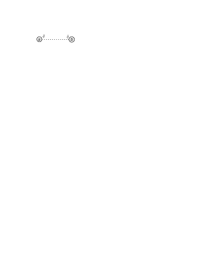
(b) No permutations necessary.

(c) 2 permutations from swapping $a\leftrightarrow b$.

(d) 2 permutations from swapping $a\leftrightarrow b$.

(e) 2 permutations from swapping $a\leftrightarrow b$.

(f) 2 permutations from swapping $a\leftrightarrow b$.

(g) No permutations necessary.

(h) 2 permutations from swapping $a\leftrightarrow b$.

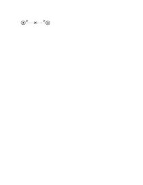
(i) No permutations necessary.

(j) 2 permutations from swapping $a\leftrightarrow b$.

Figure 4: 2 PN two body diagrams with no graviton vertices: 1 of 2

(a) 2 permutations from swapping $a\leftrightarrow b$.

(b) 2 permutations from swapping $a\leftrightarrow b$.

(c) 2 permutations from swapping $a\leftrightarrow b$.

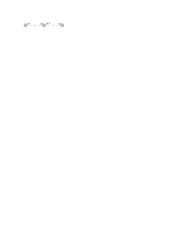
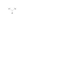
(d) 2 permutations from swapping $a\leftrightarrow b$.

(e) 2 permutations from swapping $a\leftrightarrow b$.

(f) 2 permutations from swapping $a\leftrightarrow b$.

(g) 2 permutations from swapping $a\leftrightarrow b$.

(h) No permutations necessary.

Figure 5: 2 PN two body diagrams with no graviton vertices: 2 of 2

Fig.(4$$| =i\int{\rm d}t\int\text{d}t_{a}\int\text{d}t_{b}\frac{(d-3)\Gamma\left[\frac{d-7}{2}\right]}{512\pi^{\frac{d-1}{2}}(d-2)}$$a)

$$\times\frac{M_{a}M_{b}}{M_{\text{pl}}^{d-2}R_{ab}^{d-7}}\left(\frac{\text{d}}{\text{d}t_{a}}\frac{\text{d}}{\text{d}t_{b}}\right)^{2}\delta[t-t_{a}]\delta[t-t_{b}]$$

Fig.(4$$| =i\int{\rm d}t\frac{\Gamma\left[\frac{d-3}{2}\right]}{16\pi^{\frac{d-1}{2}}}\frac{M_{a}M_{b}}{M_{\text{pl}}^{d-2}R_{ab}^{d-3}}$$b)

$$\qquad\times\left((\vec{v}_{a}\cdot\vec{v}_{b})^{2}-\frac{\vec{v}_{a}^{2}\vec{v}_{b}^{2}}{d-2}\right)$$

Fig.(4$$| =i\int{\rm d}t\frac{\Gamma\left[\frac{d-3}{2}\right]}{32\pi^{\frac{d-1}{2}}(d-2)}\frac{M_{a}M_{b}}{M_{\text{pl}}^{d-2}R_{ab}^{d-3}}\vec{v}_{a}^{2}\vec{v}_{b}^{2}$$c)

Fig.(4$$| =-i\int{\rm d}t\frac{\Gamma\left[\frac{d-3}{2}\right]}{16\pi^{\frac{d-1}{2}}}\frac{M_{a}M_{b}}{M_{\text{pl}}^{d-2}R_{ab}^{d-3}}\vec{v}_{a}\cdot\vec{v}_{b}\ \vec{v}_{a}^{2}$$d)

Fig.(4$$| =i\int{\rm d}t\frac{\Gamma\left[\frac{d-3}{2}\right]}{32(d-2)\pi^{\frac{d-1}{2}}}\frac{M_{a}M_{b}}{M_{\text{pl}}^{d-2}R_{ab}^{d-3}}\vec{v}_{a}^{4}$$e)

Fig.(4$$| =i\int{\rm d}t\frac{3\Gamma\left[\frac{d-1}{2}\right]}{64(d-2)\pi^{\frac{d-1}{2}}}\frac{M_{a}M_{b}}{M_{\text{pl}}^{d-2}R_{ab}^{d-3}}\vec{v}_{a}^{4}$$f)

Fig.(4$$| =i\int{\rm d}t\frac{\Gamma\left[\frac{d-1}{2}\right]}{32(d-2)\pi^{\frac{d-1}{2}}}\frac{M_{a}M_{b}}{M_{\text{pl}}^{d-2}R_{ab}^{d-3}}\vec{v}_{a}^{2}\vec{v}_{b}^{2}$$g)

Fig.(4$$| =i\int{\rm d}t\int\text{d}t_{a}\int\text{d}t_{b}\frac{\Gamma\left[\frac{d-5}{2}\right]}{64(d-2)\pi^{\frac{d-1}{2}}}$$h)

$$\qquad\times\frac{M_{a}M_{b}}{M_{\text{pl}}^{d-2}R_{ab}^{d-5}}\vec{v}_{a}^{2}\frac{{\rm d}}{{\rm d}t_{a}}\frac{{\rm d}}{{\rm d}t_{b}}\delta[t-t_{a}]\delta[t-t_{b}]$$

Fig.(4$$| =-i\int{\rm d}t\int\text{d}t_{a}\int\text{d}t_{b}\frac{\Gamma\left[\frac{d-5}{2}\right]}{32\pi^{\frac{d-1}{2}}}$$i)

$$\times\frac{M_{a}M_{b}}{M_{\text{pl}}^{d-2}R_{ab}^{d-5}}\vec{v}_{a}\cdot\vec{v}_{b}\frac{{\rm d}}{{\rm d}t_{a}}\frac{{\rm d}}{{\rm d}t_{b}}\delta[t-t_{a}]\delta[t-t_{b}]$$

Fig.(4$$| =i\int{\rm d}t\int\text{d}t_{a}\int\text{d}t_{b}\frac{(d-3)\Gamma\left[\frac{d-5}{2}\right]}{128(d-2)\pi^{\frac{d-1}{2}}}$$j)

$$\qquad\times\frac{M_{a}M_{b}}{M_{\text{pl}}^{d-2}R_{ab}^{d-5}}\vec{v}_{a}^{2}\frac{{\rm d}}{{\rm d}t_{a}}\frac{{\rm d}}{{\rm d}t_{b}}\delta[t-t_{a}]\delta[t-t_{b}]$$

Fig.(5$$| =i\int{\rm d}t\frac{(d-3)\Gamma\left[\frac{d-3}{2}\right]^{2}}{256(d-2)^{2}\pi^{d-1}}\frac{M_{a}M_{b}^{2}}{M_{\text{pl}}^{2(d-2)}R_{ab}^{2(d-3)}}\vec{v}_{b}^{2}$$a)

Fig.(5$$| =-i\int{\rm d}t\frac{(d-3)\Gamma\left[\frac{d-3}{2}\right]^{2}}{128(d-2)\pi^{d-1}}$$b)

$$\quad\times\frac{M_{a}M_{b}^{2}}{M_{\text{pl}}^{2(d-2)}R_{ab}^{2(d-3)}}\vec{v}_{a}\cdot\vec{v}_{b}$$

Fig.(5$$| =i\int{\rm d}t\frac{(d-3)\Gamma\left[\frac{d-3}{2}\right]^{2}}{256(d-2)^{2}\pi^{d-1}}\frac{M_{a}M_{b}^{2}}{M_{\text{pl}}^{2(d-2)}R_{ab}^{2(d-3)}}\vec{v}_{a}^{2}$$c)

Fig.(5$$| =i\int{\rm d}t\frac{3\Gamma\left[\frac{d-1}{2}\right]^{2}}{256(d-2)^{2}\pi^{d-1}}\frac{M_{a}^{2}M_{b}}{M_{\text{pl}}^{2(d-2)}R_{ab}^{2(d-3)}}\vec{v}_{b}^{2}$$d)

Fig.(5$$| =i\int{\rm d}t\frac{\Gamma\left[\frac{d-1}{2}\right]^{2}}{128(d-2)^{2}\pi^{d-1}}\frac{M_{a}^{2}M_{b}}{M_{\text{pl}}^{2(d-2)}R_{ab}^{2(d-3)}}\vec{v}_{a}^{2}$$e)

Fig.(5$|$f) contains a first order relativistic correction to the graviton Green’s function. Integrating over the time $\delta$-function with no time derivatives acting on it, before integrating by parts, the resulting integral becomes

Fig.(5$$|$$f)

$$=\frac{i(d-3)\Gamma\left[\frac{d-5}{2}\right]\Gamma\left[\frac{d-1}{2}\right]M_{a}M_{b}^{2}}{512(d-2)^{2}M_{\text{pl}}^{2(d-2)}\pi^{d-1}}\int\text{d}t_{a}\int\text{d}t_{b}\delta[t_{a}-t_{b}]$$

$$\times\bigg{(}\frac{\text{d}|\vec{x}_{b}[t_{a}]-\vec{x}_{a}[t_{a}]|^{3-d}}{\text{d}t_{a}}\frac{\text{d}|\vec{x}_{b}[t_{b}]-\vec{x}_{a}[t_{a}]|^{5-d}}{\text{d}t_{b}}$$

$$\qquad+|\vec{x}_{b}[t_{a}]-\vec{x}_{a}[t_{a}]|^{3-d}\frac{\text{d}^{2}|\vec{x}_{b}[t_{b}]-\vec{x}_{a}[t_{a}]|^{5-d}}{\text{d}t_{a}\text{d}t_{b}}\bigg{)},$$ (24)

with a common time argument $t_{a}$ for both $\vec{x}_{a}$ and $\vec{x}_{b}$ in the factor $|\dots|^{3-d}$.

Fig.(5$$| =i\int{\rm d}t\frac{\Gamma\left[\frac{d-1}{2}\right]^{3}}{1024(d-2)^{3}\pi^{\frac{3}{2}(d-1)}}\frac{M_{a}^{3}M_{b}}{M_{\text{pl}}^{3(d-2)}R_{ab}^{3(d-3)}}$$g)

Fig.(5$$| =i\int{\rm d}t\frac{\Gamma\left[\frac{d-1}{2}\right]^{3}}{512(d-2)^{3}\pi^{\frac{3}{2}(d-1)}}\frac{M_{a}^{2}M_{b}^{2}}{M_{\text{pl}}^{3(d-2)}R_{ab}^{3(d-3)}}$$h)

(a) 2 permutations from swapping $a\leftrightarrow b$.

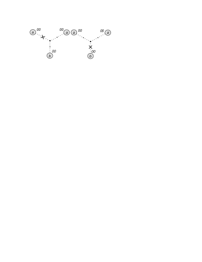
(b) 2 permutations from swapping $a\leftrightarrow b$.

(c) 2 permutations from swapping $a\leftrightarrow b$.

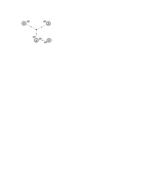
(d) 2 permutations from swapping $a\leftrightarrow b$.

Figure 6: 2 PN 2 body diagrams with graviton vertices: 1 of 4

(a) 2 permutations from swapping $a\leftrightarrow b$.

(b) 2 permutations from swapping $a\leftrightarrow b$.

(c) 2 permutations from swapping $a\leftrightarrow b$.

(d) 2 permutations from swapping $a\leftrightarrow b$.

Figure 7: 2 PN 2 body diagrams with graviton vertices: 2 of 4

(a) 2 permutations from swapping $a\leftrightarrow b$.

(b) 2 permutations from swapping $a\leftrightarrow b$.

(c) 2 permutations from swapping $a\leftrightarrow b$.

(d) 2 permutations from swapping $a\leftrightarrow b$.

Figure 8: 2 PN 2 body diagrams with graviton vertices: 3 of 4

(a) 2 permutations from swapping $a\leftrightarrow b$.

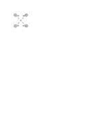
(b) No permutations necessary.

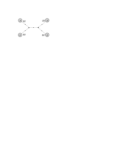
(c) 6 permutations. See text for discussion.

(d) 6 permutations. See text for discussion.

Figure 9: 2 PN 2 body diagrams with graviton vertices: 4 of 4

Graviton vertices  The rest of the 2 body diagrams contain terms from the Einstein-Hilbert action.

Note that the form of the fourier space master integrals associated with each class of diagrams usually comes about after some manipulation of momentum dot products, application of the identity $2\vec{p}_{a}\cdot\vec{p}_{b}=\mp(\vec{p}_{a}\mp\vec{p}_{b})^{2}\pm\vec{p}_{a}^{2}\pm\vec{p}_{b}^{2}$ and its analogs, and the use of momentum conservation $\sum_{r=1}^{\ell}\vec{p}_{r}=0$, $\ell=3$ or $4$.

Fig.(6$|$a, b)  The 2- and 3-body version of Fig.(6$|$a, b) requires the following master integral:

$$I_{0i0000}[q,r,s]$$

$$\equiv i\int{\rm d}t\int\text{d}t_{q}\int\text{d}t_{r}\int\text{d}t_{s}\frac{\delta[t-t_{q}]}{2(d-2)M_{\text{pl}}^{(d-2)/2}}$$

$$\times\left(\prod_{\ell=1}^{3}\int\frac{\text{d}^{d-1}p_{\ell}}{(2\pi)^{d-1}}\right)$$

$$\times\vec{v}_{a}\cdot[(2(d-4)\vec{p}_{2}+(d-5)\vec{p}_{3})$$

$$\qquad\times\delta[t-t_{s}](i(\text{d}/\text{d}t_{r})\delta[t-t_{r}])$$

$$\qquad+((d-5)\vec{p}_{2}+2(d-4)\vec{p}_{3})$$

$$\qquad\times\delta[t-t_{r}](i(\text{d}/\text{d}t_{s})\delta[t-t_{s}])]$$

$$\times\frac{\exp\left[i\left(\vec{p}_{1}\cdot\vec{x}_{q}[t_{q}]+\vec{p}_{2}\cdot\vec{x}_{r}[t_{r}]+\vec{p}_{3}\cdot\vec{x}_{s}[t_{s}]\right)\right]}{\vec{p}_{1}^{2}\vec{p}_{2}^{2}\vec{p}_{3}^{2}}$$

$$\times(2\pi)^{d-1}\delta^{d-1}\left[\vec{p}_{1}+\vec{p}_{2}+\vec{p}_{3}\right]$$ (25)

Notice that a $p_{s}^{j}$ (with $s=1,2$ or $3$) in the numerator can be obtained by differentiating the appropriate exponential, i.e. $p_{s}^{j}\exp[i\vec{p}_{s}\cdot\vec{x}_{r}]=-i(\partial/\partial x_{r}^{j})\exp[i\vec{p}_{s}\cdot\vec{x}_{r}]$. Our approach to the fourier integrals arising from this and the rest of the diagrams with graviton vertices is to first substitute the momentum $\delta$-function(s) with its (their) integral representation(s),

$$(2\pi)^{d-1}\delta^{d-1}\left[\sum_{r=1}^{s}\vec{p}_{r}\right] =\int\text{d}^{d-1}z\exp\left[-i\vec{z}\cdot\sum_{r=1}^{s}\vec{p}_{r}\right],$$ (26)

and next use (B) to re-express the original momentum integrals as position space ones, with the momentum dot products in the numerator converted into derivatives on the resulting integrand.

In this regard, the 2-distinct particles case usually requires more care than the 3- and 4-distinct particles cases. We shall illustrate this with Fig.(6$|$a), where $\vec{x}_{q}=\vec{x}_{r}\equiv\vec{x}_{a}$ and $\vec{x}_{s}\equiv\vec{x}_{b}$. The time derivatives occurring in Fig.(6$|$a) are

$$\frac{\text{d}}{\text{d}t_{a}} =v_{a}^{j}[t_{a}]\frac{\partial}{\partial x_{a}^{j}[t_{a}]},$$

$$\frac{\text{d}}{\text{d}t_{b}} =v_{a}^{j}[t_{b}]\frac{\partial}{\partial x_{a}^{j}[t_{b}]},$$

$$\frac{\text{d}}{\text{d}t_{c}} =v_{b}^{j}[t_{c}]\frac{\partial}{\partial x_{b}^{j}[t_{c}]},$$

with each partial derivative acting only on the appropriate $|\vec{x}_{a}-\vec{z}|$ or $|\vec{x}_{b}-\vec{z}|$ with the same time argument as the velocity vector contracted into it.

When $d=4-2\varepsilon$, we therefore have

Fig.(6$$|$$a)

$$=\frac{M_{a}^{2}M_{b}}{4M_{\text{pl}}^{(3/2)(d-2)}}I_{0i0000}[a,a,b]$$

$$\stackrel{{\scriptstyle d=4}}{{=}}\lim_{\varepsilon\to 0}i\int{\rm d}t\int\text{d}t_{a}\int\text{d}t_{b}\int\text{d}t_{c}\frac{M_{a}^{2}M_{b}}{16M_{\text{pl}}^{4}}$$

$$\times\delta[t-t_{a}]\delta[t-t_{b}]\delta[t-t_{c}]\left(\frac{\Gamma[(1/2)-\varepsilon]}{4\pi^{(3-2\varepsilon)/2}}\right)^{2}\int\text{d}^{3-2\varepsilon}z$$

$$\times v_{a}^{i}[t_{a}]\big{(}v_{a}^{j}[t_{b}]|\vec{x}_{a}[t_{a}]-\vec{z}|^{-1+2\varepsilon}$$

$$\qquad\times(\partial_{j}^{a}|\vec{x}_{a}[t_{b}]-\vec{z}|^{-1+2\varepsilon})(\partial_{i}^{b}|\vec{x}_{b}[t_{c}]-\vec{z}|^{-1+2\varepsilon})$$

$$\ +v_{b}^{j}[t_{c}]|\vec{x}_{a}[t_{a}]-\vec{z}|^{-1+2\varepsilon}$$

$$\qquad\times(\partial_{j}^{b}|\vec{x}_{b}[t_{c}]-\vec{z}|^{-1+2\varepsilon})(\partial_{i}^{a}|\vec{x}_{a}[t_{b}]-\vec{z}|^{-1+2\varepsilon})\big{)},$$

After differentiation, these integrals can then be evaluated using (61). This leads us to

Fig.(6$$| \stackrel{{\scriptstyle d=4}}{{=}}i\int{\rm d}t\frac{M_{a}^{2}M_{b}}{512M_{\text{pl}}^{4}\pi^{2}R_{ab}^{4}}$$a)

$$\times(-2(\vec{R}_{ab}\cdot\vec{v}_{a})^{2}-2\vec{R}_{ab}\cdot\vec{v}_{b}\ \vec{R}_{ab}\cdot\vec{v}_{a}$$

$$\qquad+(\vec{v}_{a}^{2}+\vec{v}_{a}\cdot\vec{v}_{b})R_{ab}^{2})$$

A similar analysis for Fig.(6$|$b), making use of (B) and (60), gives

Fig.(6$$| =\frac{M_{a}M_{b}^{2}}{8M_{\text{pl}}^{(3/2)(d-2)}}I_{0i0000}[a,b,b]$$b)

$$\stackrel{{\scriptstyle d=4}}{{=}}i\int{\rm d}t\frac{M_{a}M_{b}^{2}}{1024M_{\text{pl}}^{4}\pi^{2}R_{ab}^{4}}$$

$$\times\left(\vec{R}_{ba}\cdot\vec{v}_{a}\ \vec{R}_{ba}\cdot\vec{v}_{b}-\vec{v}_{a}\cdot\vec{v}_{b}\ R_{ab}^{2}\right)$$

Before proceeding further, it is useful to introduce the following master integral that would occur in several 2-, 3- and 4-body Feynman integrals:

$$I_{3}[a,b,c]$$

$$=\left(\prod_{s=1}^{3}\int\frac{{\rm d}^{d-1}p_{s}}{(2\pi)^{d-1}}\right)(2\pi)^{d-1}\delta^{(d-1)}\left[\vec{p}_{1}+\vec{p}_{2}+\vec{p}_{3}\right]$$

$$\quad\times\frac{\exp\left[i\left(\vec{p}_{1}\cdot\vec{x}_{a}+\vec{p}_{2}\cdot\vec{x}_{b}+\vec{p}_{3}\cdot\vec{x}_{c}\right)\right]}{\vec{p}_{1}^{2}\vec{p}_{2}^{2}\vec{p}_{3}^{2}}$$

$$=\left(\frac{\Gamma\left[\frac{d-3}{2}\right]}{4\pi^{\frac{d-1}{2}}}\right)^{3}\int\frac{{\rm d}^{d-1}z}{|\vec{z}-\vec{x}_{a}|^{d-3}|\vec{z}-\vec{x}_{b}|^{d-3}|\vec{z}-\vec{x}_{c}|^{d-3}},$$ (27)

where we have provided both its fourier and position space representations. In appendix B, we obtain $I_{3}[a,b,c]$ in closed form when $d=4-2\varepsilon$, up to $\mathcal{O}[\varepsilon^{0}]$ (B).

Fig.(6$|$c,d)  We now turn to Fig.(6$|$c) and Fig.(6$|$d). Its associated master integral is

$$I_{ij0000}[q,r,s]$$

$$\equiv i\int{\rm d}t\int\text{d}t_{q}\int\text{d}t_{r}\int\text{d}t_{s}\frac{\delta[t-t_{q}]\delta[t-t_{r}]\delta[t-t_{s}]}{M_{\text{pl}}^{(d-2)/2}}$$

$$\times\left(\prod_{\ell=1}^{3}\int\frac{\text{d}^{d-1}p_{\ell}}{(2\pi)^{d-1}}\right)$$

$$\times\bigg{\{}\frac{\vec{v}_{q}^{2}}{(d-2)^{2}}\frac{\vec{p}_{1}^{2}-(d-3)(\vec{p}_{2}^{2}+\vec{p}_{3}^{2})}{\vec{p}_{1}^{2}\vec{p}_{2}^{2}\vec{p}_{3}^{2}}$$

$$\qquad+\frac{d-3}{2(d-2)}\frac{(\vec{p}_{1}\cdot\vec{v}_{q})^{2}+(\vec{p}_{2}\cdot\vec{v}_{q})^{2}+(\vec{p}_{3}\cdot\vec{v}_{q})^{2}}{\vec{p}_{1}^{2}\vec{p}_{2}^{2}\vec{p}_{3}^{2}}\bigg{\}}$$

$$\times\exp\left[i\left(\vec{p}_{1}\cdot\vec{x}_{q}[t_{q}]+\vec{p}_{2}\cdot\vec{x}_{r}[t_{r}]+\vec{p}_{3}\cdot\vec{x}_{s}[t_{s}]\right)\right]$$

$$\times(2\pi)^{d-1}\delta^{d-1}\left[\vec{p}_{1}+\vec{p}_{2}+\vec{p}_{3}\right]$$ (28)

The term proportional to $\vec{v}_{q}^{2}$ may be integrated in arbitrary $d$-dimensions by integrating over the momentum that is absent in the denominator (after cancelation), followed by an application of (B), because it reduces to a product of the form $\prod_{s}(2\pi)^{1-d}\int\text{d}^{d-1}p_{s}\exp[i\vec{p}_{s}\cdot\vec{R}_{su}]/\vec{p}_{s}^{2}$. This type of fourier integral will occur frequently.

The second term containing momenta dotted into velocities has the position space representation

$$-i\frac{d-3}{2(d-2)M_{\text{pl}}^{(d-2)/2}}\int\text{d}t\left(\frac{\Gamma\left[\frac{d-3}{2}\right]}{4\pi^{\frac{d-1}{2}}}\right)^{3}$$

$$\times\int\text{d}^{d-1}z\ v_{q}^{i}v_{q}^{j}\big{(}(\partial_{i}^{p}\partial_{j}^{p}R_{pz}^{3-d})R_{qz}^{3-d}R_{rz}^{3-d}$$

$$\qquad+R_{pz}^{3-d}(\partial_{i}^{q}\partial_{j}^{q}R_{qz}^{3-d})R_{rz}^{3-d}$$

$$\qquad+R_{pz}^{3-d}R_{qz}^{3-d}(\partial_{i}^{r}\partial_{j}^{r}R_{rz}^{3-d})\big{)}$$ (29)

There is a subtlety when taking double spatial derivatives on a single factor of the Euclidean distance raised to the $3-d$ power occurring within the Feynman integrals, such as $\partial_{i}^{a}\partial_{j}^{a}R_{az}^{3-d}$. Strictly speaking, because $R_{az}^{3-d}$ is the Green’s function of the spatial laplacian operator $\delta^{ij}\partial_{i}^{a}\partial_{j}^{a}$, one needs to employ the formula

$$\frac{\partial}{\partial x^{i}}\frac{\partial}{\partial x^{j}}\frac{\Gamma\left[\frac{d-3}{2}\right]}{4\pi^{(d-1)/2}|\vec{x}|^{d-3}}$$

$$=\frac{\Gamma\left[\frac{d-1}{2}\right]}{2\pi^{(d-1)/2}}\left((d-1)\frac{x^{i}x^{j}}{|\vec{x}|^{d+1}}-\frac{\delta^{ij}}{|\vec{x}|^{d-1}}\right)$$

$$\qquad\qquad-\frac{\delta^{ij}}{d-1}\delta^{d-1}\left[\vec{x}\right],$$

where there is a $\delta$-function term in addition to those following from straightforward differentiation so that one would obtain the correct result upon taking the trace of both sides. Insofar as the Feynman integrals are concerned, however, it appears the $\delta$-function term may be dropped as long as proper regularization is used. For instance, if we try to compute the integral

$$\int\text{d}^{D-1}zR_{bz}^{-\rho}\partial_{i}^{a}\partial_{j}^{a}R_{az}^{3-d}$$

by first carrying out the differentiation (without including the $\delta$-function term), we would obtain two terms, one with a $R_{az}^{i}R_{az}^{j}$ in the integrand and the other with $\delta^{ij}$. If we simply set $D=d$ and employ the formulae (B) and (60), each of the two terms will be ill-defined. However, displacing $D=d+\kappa$ in (B) and (60), and performing a laurent expansion in $\kappa$ afterwards would yield a finite result that is not traceless and is furthermore consistent with first doing the scalar integral (B) with $\sigma_{1}=\rho$ and $\sigma_{2}=d-3$ and then carrying out the double derivatives at the end.

If one is interested only in the higher PN 2-body problem, the existence of such subtleties may be reason to stay within fourier space as far as possible for the evaluation of Feynman integrals. For the 2 body case of the integrals (III.3.1) and analogous ones below, to avoid this subtlety for the terms where there are 2 factors of $R_{az}^{3-d}$ (or 2 factors of $R_{bz}^{3-d}$) and the derivatives are acting on the $R_{bz}^{3-d}$ (or $R_{az}^{3-d}$), we shall first do the integral using $I_{3}$, before differentiation.

Along this line, we further remark that

$$\int\text{d}^{d-1}zR_{az}^{2(3-d)}\partial_{i}^{b}\partial_{j}^{b}R_{bz}^{3-d}$$

can be integrated and then differentiated, whereas

$$\int\text{d}^{d-1}zR_{az}^{3-d}R_{bz}^{3-d}\partial_{i}^{b}\partial_{j}^{b}R_{bz}^{3-d}$$

has to be differentiated first. One cannot begin with 3 distinct coordinate vectors $\{\vec{x}_{a},\vec{x}_{b},\vec{x}_{c}\}$ in this integral, engage $I_{3}$, and then set $\vec{x}_{c}=\vec{x}_{b}$: the last step involves terms like $\lim_{c\to b}R_{bc}^{i}/R_{bc}$ and $\lim_{c\to b}R_{bc}^{-2}$ and hence is ill defined.

We now employ (B), derivatives on $I_{3}$, (B) and (60) to deduce

Fig.(6$$|$$c)

$$=\frac{M_{a}^{2}M_{b}}{8M_{\text{pl}}^{(3/2)(d-2)}}I_{ij0000}[a,a,b]$$

$$\stackrel{{\scriptstyle d=4}}{{=}}i\int{\rm d}t\frac{M_{a}^{2}M_{b}}{1024M_{\text{pl}}^{4}\pi^{2}R_{ab}^{4}}$$

$$\times\left(-3(\vec{R}_{ab}\cdot\vec{v}_{a})^{2}-4(\vec{R}_{ba}\cdot\vec{v}_{a})^{2}+\vec{v}_{a}^{2}\ R_{ab}^{2}\right),$$

and

Fig.(6$$|$$d)

$$=\frac{M_{a}M_{b}^{2}}{16M_{\text{pl}}^{(3/2)(d-2)}}I_{ij0000}[a,b,b]$$

$$\stackrel{{\scriptstyle d=4}}{{=}}i\int{\rm d}t\frac{M_{a}M_{b}^{2}}{2048M_{\text{pl}}^{4}\pi^{2}R_{ab}^{4}}$$

$$\times\left(-4(\vec{R}_{ab}\cdot\vec{v}_{a})^{2}-3(\vec{R}_{ba}\cdot\vec{v}_{a})^{2}+5\vec{v}_{a}^{2}\ R_{ab}^{2}\right)$$

Fig.(7$|$a)  It turns out Fig.(7$|$a) and its 3-body counterpart are zero in $d=4$ spacetime dimensions. Because it is not apparent, we display the results here for the 3 body case. In terms of the master integral in (III.3.1), we have

Fig.(11$$|$$c)

$$=-i\int{\rm d}t\int{\rm d}t_{a}\int{\rm d}t_{b}\int{\rm d}t_{c}$$

$$\quad\times\frac{(d-4)(d-1)M_{a}M_{b}M_{c}}{16(d-2)^{2}M_{\text{pl}}^{2(d-2)}}I_{3}[a,b,c]$$

$$\quad\times\left(-\left(\frac{{\rm d}}{{\rm d}t_{a}}\right)^{2}-\left(\frac{{\rm d}}{{\rm d}t_{b}}\right)^{2}-\left(\frac{{\rm d}}{{\rm d}t_{c}}\right)^{2}\right)$$

$$\quad\times\delta[t_{a}-t]\delta[t_{b}-t]\delta[t_{c}-t]$$ (30)

To be sure, when the number of distinct particles changes from 3 to 2, the integrals occurring in Fig.(7$|$a) would be different from that in (III.3.1) – which really is the result for Fig.(11$|$c) – but because it remains finite, Fig.(7$|$a) still vanishes due to the coefficient $(d-4)$.

Fig.(7$|$b)  Fig.(7$|$b) corresponds to the first relativistic correction to each of the lowest order graviton Green’s functions in the 1 PN 3-graviton diagram Fig.(2$|$d). Its associated master integral is

$$I_{000000\times}[q,r,s]$$

$$\equiv i\int{\rm d}t\int\text{d}t_{q}\int\text{d}t_{r}\int\text{d}t_{s}\frac{(d-3)^{2}}{(d-2)^{2}M_{\text{pl}}^{(d-2)/2}}$$

$$\times\left(\prod_{\ell=1}^{3}\int\frac{\text{d}^{d-1}p_{\ell}}{(2\pi)^{d-1}}\right)$$

$$\times\bigg{\{}\frac{\vec{p}_{1}^{2}+\vec{p}_{2}^{2}+\vec{p}_{3}^{2}}{\vec{p}_{1}^{4}\vec{p}_{2}^{2}\vec{p}_{3}^{2}}\delta[t-t_{r}]\delta[t-t_{s}]\left(\frac{\text{d}^{2}}{\text{d}t_{q}^{2}}\delta[t-t_{q}]\right)$$

$$\quad+\frac{\vec{p}_{1}^{2}+\vec{p}_{2}^{2}+\vec{p}_{3}^{2}}{\vec{p}_{1}^{2}\vec{p}_{2}^{4}\vec{p}_{3}^{2}}\delta[t-t_{q}]\delta[t-t_{s}]\left(\frac{\text{d}^{2}}{\text{d}t_{r}^{2}}\delta[t-t_{r}]\right)$$

$$\quad+\frac{\vec{p}_{1}^{2}+\vec{p}_{2}^{2}+\vec{p}_{3}^{2}}{\vec{p}_{1}^{2}\vec{p}_{2}^{2}\vec{p}_{3}^{4}}\delta[t-t_{q}]\delta[t-t_{r}]\left(\frac{\text{d}^{2}}{\text{d}t_{s}^{2}}\delta[t-t_{s}]\right)\bigg{\}}$$

$$\times\exp\left[i\left(\vec{p}_{1}\cdot\vec{x}_{q}[t_{q}]+\vec{p}_{2}\cdot\vec{x}_{r}[t_{r}]+\vec{p}_{3}\cdot\vec{x}_{s}[t_{s}]\right)\right]$$

$$\times(2\pi)^{d-1}\delta^{d-1}\left[\vec{p}_{1}+\vec{p}_{2}+\vec{p}_{3}\right]$$ (31)

For the case of 2 distinct particles, $I_{000000\times}[a,a,b]$ becomes

$$I_{000000\times}[a,a,b]$$

$$\stackrel{{\scriptstyle d=4}}{{=}}\frac{i}{128\pi^{3}M_{\text{pl}}}\int\text{d}t\int\text{d}^{3-2\varepsilon}zR_{az}^{-1+2\varepsilon}R_{bz}^{-1+2\varepsilon}$$

$$\qquad\times\left(\dot{v}_{a}^{i}\partial_{i}^{a}+v_{a}^{i}v_{a}^{j}\partial_{i}^{a}\partial_{j}^{a}\right)R_{az}^{-1+2\varepsilon}$$

$$+\frac{i}{2M_{\text{pl}}}\int\text{d}t\int\text{d}t_{a}\int\text{d}t_{b}\int\text{d}t_{c}$$

$$\times\delta[t-t_{a}]\delta[t-t_{b}]\delta[t-t_{c}]$$

$$\times\int\int\frac{\text{d}^{3-2\varepsilon}p_{1}\ \text{d}^{3-2\varepsilon}p_{2}}{(2\pi)^{2(3-2\varepsilon)}}\bigg{(}\frac{e^{i\vec{p}_{2}\cdot(\vec{x}_{a}[t_{b}]-\vec{x}_{b}[t_{c}])}}{\vec{p}_{2}^{2}}$$

$$\times\frac{\dot{i\vec{v}}_{a}[t_{a}]\cdot\vec{p}_{1}-\vec{v}_{a}[t_{a}]\cdot\vec{p}_{1}\ \vec{v}_{a}[t_{a}]\cdot\vec{p}_{1}}{\vec{p}_{1}^{4}}e^{i\vec{p}_{1}\cdot(\vec{x}_{a}[t_{a}]-\vec{x}_{a}[t_{b}])}\bigg{)}$$

$$-\int\text{d}t\frac{i}{64\pi^{2}M_{\text{pl}}R_{ab}}\left(\dot{v}_{a}^{i}\partial_{i}^{a}+v_{a}^{i}v_{a}^{j}\partial_{i}^{a}\partial_{j}^{a}\right)R_{ab}$$

$$+\int\text{d}t\frac{i}{4M_{\text{pl}}}\left(\dot{v}_{b}^{i}\partial_{i}^{b}+v_{b}^{i}v_{b}^{j}\partial_{i}^{b}\partial_{j}^{b}\right)I_{3}[a,a,b].$$

The first position space integral can be evaluated using (B), (59) and (60). The fourier integral after it vanishes upon integrating over the time $\delta$-functions because the exponential becomes unity. We thus have

Fig.(7$$|$$b)

$$=\frac{M_{a}^{2}M_{b}}{16M_{\text{pl}}^{\frac{3}{2}(d-2)}}I_{000000\times}[a,a,b]$$

$$\stackrel{{\scriptstyle d=4}}{{=}}i\int{\rm d}t\frac{M_{a}^{2}M_{b}}{2048M_{\text{pl}}^{4}\pi^{2}R_{ab}^{4}}$$

$$\times\bigg{(}5(\vec{R}_{ab}\cdot\vec{v}_{a})^{2}+4(\vec{R}_{ba}\cdot\vec{v}_{b})^{2}$$

$$\quad-(4\vec{R}_{ab}\cdot\dot{\vec{v}}_{a}+2\vec{R}_{ba}\cdot\dot{\vec{v}}_{b}+3\vec{v}_{a}^{2}+2\vec{v}_{b}^{2})R_{ab}^{2}\bigg{)}$$

Fig.(7$|$c,d)  The master integral associated with Fig.(7$|$c) and Fig.(7$|$d) is

$$I_{0i0j00}[q,r,s]$$

$$\equiv i\int{\rm d}t\int\text{d}t_{q}\int\text{d}t_{r}\int\text{d}t_{s}\frac{\delta[t-t_{q}]\delta[t-t_{r}]\delta[t-t_{s}]}{4(d-2)M_{\text{pl}}^{(d-2)/2}}$$

$$\times\left(\prod_{\ell=1}^{3}\int\frac{\text{d}^{d-1}p_{\ell}}{(2\pi)^{d-1}}\right)$$

$$\times\bigg{\{}\vec{v}_{q}\cdot\vec{v}_{r}\frac{(d-4)(\vec{p}_{1}^{2}+\vec{p}_{2}^{2})+(d-2)\vec{p}_{3}^{2}}{\vec{p}_{1}^{2}\vec{p}_{2}^{2}\vec{p}_{3}^{2}}$$

$$\qquad+2(d-4)\frac{\vec{p}_{2}\cdot\vec{v}_{q}\ \vec{p}_{1}\cdot\vec{v}_{r}}{\vec{p}_{1}^{2}\vec{p}_{2}^{2}\vec{p}_{3}^{2}}$$

$$\qquad+2(d-3)\frac{\vec{p}_{3}\cdot\vec{v}_{q}\ \vec{p}_{1}\cdot\vec{v}_{r}+\vec{p}_{2}\cdot\vec{v}_{q}\ \vec{p}_{3}\cdot\vec{v}_{r}}{\vec{p}_{1}^{2}\vec{p}_{2}^{2}\vec{p}_{3}^{2}}\bigg{\}}$$

$$\times\exp\left[i\left(\vec{p}_{1}\cdot\vec{x}_{q}[t_{q}]+\vec{p}_{2}\cdot\vec{x}_{r}[t_{r}]+\vec{p}_{3}\cdot\vec{x}_{s}[t_{s}]\right)\right]$$

$$\times(2\pi)^{d-1}\delta^{d-1}\left[\vec{p}_{1}+\vec{p}_{2}+\vec{p}_{3}\right]$$ (32)

A similar approach to the one taken for (III.3.1) and (III.3.1), together with the integrals (60) and (61), then yields

Fig.(7$$|$$c)

$$=\frac{M_{a}^{2}M_{b}}{2M_{\text{pl}}^{(3/2)(d-2)}}I_{0i0j00}[a,b,a]$$

$$\stackrel{{\scriptstyle d=4}}{{=}}-i\int{\rm d}t\frac{M_{a}^{2}M_{b}}{512M_{\text{pl}}^{4}\pi^{2}R_{ab}^{4}}$$

$$\times\left(\vec{v}_{a}\cdot\vec{v}_{b}\ R_{ab}^{2}+\vec{R}_{ab}\cdot\vec{v}_{a}\ \vec{R}_{ab}\cdot\vec{v}_{b}-4\vec{R}_{ba}\cdot\vec{v}_{a}\ \vec{R}_{ba}\cdot\vec{v}_{b}\right),$$

as well as

Fig.(7$$| =\frac{M_{a}^{2}M_{b}}{4M_{\text{pl}}^{(3/2)(d-2)}}I_{0i0j00}[a,a,b]$$d)

$$\stackrel{{\scriptstyle d=4}}{{=}}i\int{\rm d}t\frac{M_{a}^{2}M_{b}}{128M_{\text{pl}}^{4}\pi^{2}R_{ab}^{4}}(\vec{R}_{ab}\cdot\vec{v}_{a})^{2}$$

Fig.(8$|$a,b)  Fig.(8$|$a) and Fig.(8$|$b) are, up to numerical constants, products of $\vec{v}_{a}^{2}$ with the 1 PN 3-graviton diagram Fig.(2$|$d), namely,

Fig.(8$$|$$a)

$$=\frac{M_{a}^{2}M_{b}}{16M_{\text{pl}}^{\frac{3}{2}(d-2)}}\int\text{d}t\ \vec{v}_{a}^{2}I_{000000}[a,b,a]$$

$$=-i\int{\rm d}t\frac{(d-3)^{2}\Gamma\left[\frac{d-3}{2}\right]^{2}M_{a}^{2}M_{b}}{256(d-2)^{2}M_{\text{pl}}^{2d-4}\pi^{d-1}R_{ab}^{2(d-3)}}\vec{v}_{a}^{2},$$

and

Fig.(8$$| =\frac{M_{a}^{2}M_{b}}{32M_{\text{pl}}^{\frac{3}{2}(d-2)}}\int\text{d}t\ \vec{v}_{b}^{2}I_{000000}[a,a,b]$$b)

$$=-i\int{\rm d}t\frac{(d-3)^{2}\Gamma\left[\frac{d-3}{2}\right]^{2}M_{a}^{2}M_{b}}{512(d-2)^{2}M_{\text{pl}}^{2(d-2)}\pi^{d-1}R_{ab}^{2(d-3)}}\vec{v}_{b}^{2}$$

Fig.(8$|$c,d)  Fig.(8$|$c) and Fig.(8$|$d) are, up to constant factors, the product of the lowest order graviton Green’s function $\langle h_{00}h_{00}\rangle$ with the 1 PN 3-graviton diagram Fig.(2$|$d), namely,

Fig.(8$$|$$c)

$$=\int\text{d}t\frac{\Gamma\left[\frac{d-1}{2}\right]M_{a}^{3}M_{b}}{128(d-2)M_{\text{pl}}^{\frac{5}{2}(d-2)}\pi^{\frac{d-1}{2}}R_{ab}^{d-3}}I_{000000}[a,a,b]$$

$$=-i\int{\rm d}t\frac{\Gamma\left[\frac{d-1}{2}\right]^{3}M_{a}^{3}M_{b}}{512(d-2)^{3}M_{\text{pl}}^{3(d-2)}\pi^{\frac{3}{2}(d-1)}R_{ab}^{3(d-3)}}$$

Fig.(8$$|$$d)

$$=\int\text{d}t\frac{\Gamma\left[\frac{d-1}{2}\right]M_{a}^{2}M_{b}^{2}}{64(d-2)M_{\text{pl}}^{\frac{5}{2}(d-2)}\pi^{\frac{d-1}{2}}R_{ab}^{d-3}}I_{000000}[a,b,b]$$

$$=-i\int{\rm d}t\frac{\Gamma\left[\frac{d-1}{2}\right]^{3}M_{a}^{2}M_{b}^{2}}{256(d-2)^{3}M_{\text{pl}}^{3(d-2)}\pi^{\frac{3}{2}(d-1)}R_{ab}^{3(d-3)}}$$

Fig.(9$|$a,b)  The associated master integral for Fig.(9$|$a) and Fig.(9$|$b) is

$$I_{00000000}[q,r,s,u]$$

$$=-i\int\text{d}t\int\text{d}t_{q}\int\text{d}t_{r}\int\text{d}t_{s}\int\text{d}t_{u}$$

$$\times\delta[t-t_{q}]\delta[t-t_{r}]\delta[t-t_{s}]\delta[t-t_{u}]$$

$$\times\frac{(d-3)(d(7d-51)+86)}{4(d-2)^{3}M_{\text{pl}}^{d-2}}\left(\prod_{\ell=1}^{4}\int\frac{\text{d}^{d-1}p_{\ell}}{(2\pi)^{d-1}}\right)$$

$$\times\frac{\vec{p}_{1}^{2}+\vec{p}_{2}^{2}+\vec{p}_{3}^{2}+\vec{p}_{4}^{2}}{\vec{p}_{1}^{2}\vec{p}_{2}^{2}\vec{p}_{3}^{2}\vec{p}_{4}^{2}}$$

$$\times\exp\left[i\left(\vec{p}_{1}\cdot\vec{x}_{q}+\vec{p}_{2}\cdot\vec{x}_{r}+\vec{p}_{3}\cdot\vec{x}_{s}+\vec{p}_{4}\cdot\vec{x}_{u}\right)\right]$$

$$\times(2\pi)^{d-1}\delta^{d-1}\left[\vec{p}_{1}+\vec{p}_{2}+\vec{p}_{3}+\vec{p}_{4}\right]$$ (33)

Employing (B) hands us

Fig.(9$$|$$a)

$$=\frac{M_{a}^{3}M_{b}}{96M_{\text{pl}}^{2(d-2)}}I_{00000000}[a,a,a,b]$$

$$=-i\int{\rm d}t\frac{(d-3)(d(7d-51)+86)\Gamma^{3}\left[\frac{d-3}{2}\right]M_{a}^{3}M_{b}}{24576(d-2)^{3}M_{\text{pl}}^{3(d-2)}\pi^{\frac{3}{2}(d-1)}R_{ab}^{3(d-3)}}$$

and

Fig.(9$$| =\frac{M_{a}^{2}M_{b}^{2}}{64M_{\text{pl}}^{2(d-2)}}I_{00000000}[a,a,b,b]$$b)

$$=0$$

Fig.(9$|$c,d)  The evaluation of Fig.(9$|$c) and Fig.(9$|$d), involving the contraction of 2 3-graviton vertices, requires the most effort. Its associated master integrals in momentum space, after substantial algebraic manipulation reads:

$$I_{0000-0000}[q,r,s,u]=I_{0000-0000}^{\text{I}}[q,r,s,u]+I_{0000-0000}^{\text{II}}[q,r,s,u]+I_{0000-0000}^{\text{III}}[q,r,s,u]$$ (34)

$$I_{0000-0000}^{\text{I}}[q,r,s,u]$$ (35)

$$\equiv i\int{\rm d}t\int\text{d}t_{q}\int\text{d}t_{r}\int\text{d}t_{s}\int\text{d}t_{u}\frac{\delta[t-t_{q}]\delta[t-t_{r}]\delta[t-t_{s}]\delta[t-t_{u}]}{8(d-2)^{3}M_{\text{pl}}^{d-2}}\left(\prod_{\ell=1}^{4}\int\frac{\text{d}^{d-1}p_{\ell}}{(2\pi)^{d-1}}\right)$$

$$\quad\times\frac{1}{\vec{p}_{1}^{2}\vec{p}_{2}^{2}\vec{p}_{3}^{2}\vec{p}_{4}^{2}}\bigg{\{}(d-3)^{2}(5d-18)\left(\vec{p}_{1}^{2}+\vec{p}_{2}^{2}+\vec{p}_{3}^{2}+\vec{p}_{4}^{2}\right)+(3d^{3}-40d^{2}+151d-174)(\vec{p}_{1}+\vec{p}_{2})^{2}$$

$$\qquad\qquad-\frac{(d-3)^{2}}{(\vec{p}_{1}+\vec{p}_{2})^{2}}\left(4(d-2)(\vec{p}_{1}^{2}\vec{p}_{2}^{2}+\vec{p}_{3}^{2}\vec{p}_{4}^{2})-(7d-22)(\vec{p}_{1}^{2}+\vec{p}_{2}^{2})(\vec{p}_{3}^{2}+\vec{p}_{4}^{2})\right)\bigg{\}}$$

$$\quad\times\exp\big{[}i\vec{p}_{1}\cdot\vec{x}_{q}[t_{q}]+i\vec{p}_{2}\cdot\vec{x}_{r}[t_{r}]+i\vec{p}_{3}\cdot\vec{x}_{s}[t_{s}]+i\vec{p}_{4}\cdot\vec{x}_{u}[t_{u}]\big{]}(2\pi)^{d-1}\delta^{d-1}\left[\sum_{w=1}^{4}\vec{p}_{w}\right]$$

$$+\text{5 other permutations of }\{\vec{x}_{q},\vec{x}_{r},\vec{x}_{s},\vec{x}_{u}\}$$

$$I_{0000-0000}^{\text{II}}[q,r,s,u]$$ (36)

$$\equiv i\int{\rm d}t\int\text{d}t_{q}\int\text{d}t_{r}\int\text{d}t_{s}\int\text{d}t_{u}\frac{(d-3)^{2}\delta[t-t_{q}]\delta[t-t_{r}]\delta[t-t_{s}]\delta[t-t_{u}]}{4(d-2)^{2}M_{\text{pl}}^{d-2}}\left(\prod_{\ell=1}^{4}\int\frac{\text{d}^{d-1}p_{\ell}}{(2\pi)^{d-1}}\right)$$

$$\quad\times\frac{\vec{p}_{1}^{4}+\vec{p}_{2}^{4}+\vec{p}_{3}^{4}+\vec{p}_{4}^{4}}{\vec{p}_{1}^{2}\vec{p}_{2}^{2}\vec{p}_{3}^{2}\vec{p}_{4}^{2}(\vec{p}_{1}+\vec{p}_{2})^{2}}\exp\left[i\vec{p}_{1}\cdot\vec{x}_{q}[t_{q}]+i\vec{p}_{2}\cdot\vec{x}_{r}[t_{r}]+i\vec{p}_{3}\cdot\vec{x}_{s}[t_{s}]+i\vec{p}_{4}\cdot\vec{x}_{u}[t_{u}]\right](2\pi)^{d-1}\delta^{d-1}\left[\sum_{w=1}^{4}\vec{p}_{w}\right]$$

$$+\text{5 other permutations of }\{\vec{x}_{q},\vec{x}_{r},\vec{x}_{s},\vec{x}_{u}\}$$

$$I_{0000-0000}^{\text{III}}[q,r,s,u]$$ (37)

$$\equiv i\int{\rm d}t\int\text{d}t_{q}\int\text{d}t_{r}\int\text{d}t_{s}\int\text{d}t_{u}\frac{(d-3)^{2}\delta[t-t_{q}]\delta[t-t_{r}]\delta[t-t_{s}]\delta[t-t_{u}]}{2(d-2)^{2}M_{\text{pl}}^{d-2}}\left(\prod_{\ell=1}^{4}\int\frac{\text{d}^{d-1}p_{\ell}}{(2\pi)^{d-1}}\right)$$

$$\times\frac{\vec{p}_{1}\cdot\vec{p}_{3}\ \vec{p}_{2}\cdot\vec{p}_{4}+\vec{p}_{1}\cdot\vec{p}_{4}\ \vec{p}_{2}\cdot\vec{p}_{3}}{\vec{p}_{1}^{2}\vec{p}_{2}^{2}\vec{p}_{3}^{2}\vec{p}_{4}^{2}(\vec{p}_{1}+\vec{p}_{2})^{2}}\exp\left[i\vec{p}_{1}\cdot\vec{x}_{q}[t_{q}]+i\vec{p}_{2}\cdot\vec{x}_{r}[t_{r}]+i\vec{p}_{3}\cdot\vec{x}_{s}[t_{s}]+i\vec{p}_{4}\cdot\vec{x}_{u}[t_{u}]\right](2\pi)^{d-1}\delta^{d-1}\left[\sum_{w=1}^{4}\vec{p}_{w}\right]$$

$$+\text{5 other permutations of }\{\vec{x}_{q},\vec{x}_{r},\vec{x}_{s},\vec{x}_{u}\}$$

When contracting the 2 3-graviton Feynman rules in momentum space leading to (34,35,36,37), one makes a particular choice for the labels on the point particles’ coordinate vectors. If the two particle labels on the 3-graviton vertex on the left hand side are $\{a,b\}$ and the two on the right hand side are $\{c,e\}$, so that such a choice can be denoted as either $(ab|ce)$, $(ba|ce)$, $(ab|ec)$ or $(ba|ec)$ – there is a symmetry obeyed by the labels on either side – then the 6 permutations to be summed over in the definitions of $I_{0000-0000}^{\text{I}},I_{0000-0000}^{\text{II}}$ and $I_{0000-0000}^{\text{III}}$ are: $2\times(ab|ce)$, $2\times(ac|be)$ and $2\times(ae|bc)$. The particular permutation displayed in Fig.(9$|$c) is $(aa|ba)$. It also represents the sum of the 6 permutations, with each of the 6 terms giving the same result. In our notation, the sum is $6\times(aa|ab)$. As for the two diagrams in Fig.(9$|$d), they represent the sum of the 6 permutations: $4\times(ab|ab)$ and $2\times(aa|bb)$.

Turning to the integrals themselves, $I_{0000-0000}^{\text{I}}[q,r,s,u]$ can be calculated in $d$-dimensions with (B). For the term containing $(\vec{p}_{1}+\vec{p}_{2})^{2}$ in the numerator, one would first sum over the 6 permutations of the coordinate vectors $\{\vec{x}_{q}\}$; this is equivalent to holding fixed the $\{\vec{x}_{q},\vec{x}_{r},\vec{x}_{s},\vec{x}_{u}\}$ and permuting the names of the integration variables $\{\vec{p}_{1},\dots,\vec{p}_{4}\}$. Upon doing so, one would find the relevant part of the integrand can be replaced as follows: $(\vec{p}_{1}+\vec{p}_{2})^{2}/(\vec{p}_{1}^{2}\vec{p}_{2}^{2}\vec{p}_{3}^{2}\vec{p}_{4}^{2})\to 2(\vec{p}_{1}^{2}+\vec{p}_{2}^{2}+\vec{p}_{3}^{2}+\vec{p}_{4}^{2})/(\vec{p}_{1}^{2}\vec{p}_{2}^{2}\vec{p}_{3}^{2}\vec{p}_{4}^{2})$. After suitable re-definitions of the momentum variables of the form $\vec{p}^{\prime}_{a}\equiv\vec{p}_{a}+\vec{p}_{b}$, the $(\vec{p}_{1}^{2}\vec{p}_{2}^{2}+\vec{p}_{3}^{2}\vec{p}_{4}^{2})/(\vec{p}_{1}+\vec{p}_{2})^{2}$ portion of $I_{0000-0000}^{\text{I}}[q,r,s,u]$ is, after integration, proportional to $\delta^{d-1}[\vec{x}_{q}-\vec{x}_{r}]$ or $\delta^{d-1}[\vec{0}]$, i.e. zero within dimension regularization; while the $(\vec{p}_{1}^{2}+\vec{p}_{2}^{2})(\vec{p}_{3}^{2}+\vec{p}_{4}^{2})/(\vec{p}_{1}+\vec{p}_{2})^{2}$ integrand again takes the (B)-form $\exp[i\sum_{r}^{3}\vec{p}_{r}\cdot\vec{R}_{ru}]/[\prod_{s}^{3}\vec{p}_{s}^{2}]$.

$I_{0000-0000}^{\text{II}}[q,r,s,u]$ can be dealt with by first integrating, for each of its four terms, over the momentum appearing in the numerator. We demonstrate this with the first term, dropping all numerical constants and suppressing the time arguments.

$$\left(\prod_{\ell=1}^{4}\int\frac{\text{d}^{d-1}p_{\ell}}{(2\pi)^{d-1}}\right)\frac{\vec{p}_{1}^{4}}{\vec{p}_{1}^{2}\vec{p}_{2}^{2}\vec{p}_{3}^{2}\vec{p}_{4}^{2}(\vec{p}_{1}+\vec{p}_{2})^{2}}$$

$$\times\exp\big{[}i\big{(}\vec{p}_{1}\cdot\vec{x}_{q}+\vec{p}_{2}\cdot\vec{x}_{r}+\vec{p}_{3}\cdot\vec{x}_{s}+\vec{p}_{4}\cdot\vec{x}_{u}\big{)}\big{]}$$

$$\times(2\pi)^{d-1}\delta^{d-1}\left[\vec{p}_{1}+\vec{p}_{2}+\vec{p}_{3}+\vec{p}_{4}\right]$$

$$=\left(\prod_{\ell=2}^{4}\int\frac{\text{d}^{d-1}p_{\ell}}{(2\pi)^{d-1}}\right)$$

$$\times\bigg{\{}\frac{1}{\vec{p}_{2}^{2}\vec{p}_{3}^{2}\vec{p}_{4}^{2}}e^{i\vec{p}_{2}\cdot(\vec{x}_{r}-\vec{x}_{q})+i\vec{p}_{3}\cdot(\vec{x}_{s}-\vec{x}_{q})+i\vec{p}_{4}\cdot(\vec{x}_{u}-\vec{x}_{q})}$$

$$+2\delta_{ij}\frac{p_{2}^{i}}{\vec{p}_{2}^{2}}e^{i\vec{p}_{2}\cdot(\vec{x}_{r}-\vec{x}_{q})}\frac{(p_{3}^{j}+p_{4}^{j})}{\vec{p}_{3}^{2}\vec{p}_{4}^{2}(\vec{p}_{3}+\vec{p}_{4})^{2}}$$

$$\qquad\times e^{i\vec{p}_{3}\cdot(\vec{x}_{s}-\vec{x}_{q})+i\vec{p}_{4}\cdot(\vec{x}_{u}-\vec{x}_{q})}\bigg{\}},$$ (38)

where we have dropped the term proportional to $\int\text{d}^{d-1}p_{2}\exp[i\vec{p}_{2}\cdot(\vec{x}_{r}[t_{r}]-\vec{x}_{q}[t_{q}])]$, which is zero even if $\vec{x}_{r}=\vec{x}_{q}$, within dimensional regularization. The first piece in the second equality containing only squares of momenta in the denominator can be done with (B). For the second piece, the $\vec{p}_{2}$ integral is a $(1/i)\partial_{i}^{r}$ on $(\ref{integral_PropI})$; it is zero if $\vec{x}_{r}=\vec{x}_{q}$. The $\vec{p}_{3}$ and $\vec{p}_{4}$ integrals translate to an appropriate derivative on $I_{3}[a,a,b]$ or $I_{3}[a,b,b]$ if $\vec{x}_{s}=\vec{x}_{u}$ and $\vec{x}_{s}\neq\vec{x}_{q}$. If $\vec{x}_{s}=\vec{x}_{q}$ and $\vec{x}_{u}\neq\vec{x}_{q}$ (or vice versa), the $\vec{p}_{3}$ ($\vec{p}_{4}$) integrals take the form of (59), and the remaining $\vec{p}_{4}$ ($\vec{p}_{3}$) integral is then a derivative on (B). The $\vec{p}_{3}$ and $\vec{p}_{4}$ integrals return zero if $\vec{x}_{s}=\vec{x}_{u}=\vec{x}_{q}$.

What remains is $I_{0000-0000}^{\text{III}}[q,r,s,u]$. First replace the $(\vec{p}_{1}+\vec{p}_{2})^{2}$ in the denominator with $\vec{q}$ and introduce a $(2\pi)^{1-d}\int\text{d}^{d-1}q\delta^{(d-1)}[\vec{q}-\vec{p}_{1}-\vec{p}_{2}]$. Applying (26) on both the $\delta$-functions then tells us that, in its position space representation – again ignoring the constant factors – $I_{0000-0000}^{\text{III}}[q,r,s,u]$ becomes

$$\int\text{d}^{d-1}y\int\text{d}^{d-1}z\ \delta^{ij}\delta^{mn}$$

$$\times\big{(}(\partial_{i}^{q}R_{qy}^{3-d})(\partial_{m}^{r}R_{ry}^{3-d})(R_{yz}^{3-d})(\partial_{j}^{s}R_{sz}^{3-d})(\partial_{n}^{u}R_{uz}^{3-d})$$

$$\quad+(\partial_{i}^{q}R_{qy}^{3-d})(\partial_{m}^{r}R_{ry}^{3-d})(R_{yz}^{3-d})(\partial_{n}^{s}R_{sz}^{3-d})(\partial_{j}^{u}R_{uz}^{3-d})\big{)}$$

For the 2 body problem, we would either have one of the $\vec{y}$ or $\vec{z}$ integration involve only one of the coordinate vectors $\vec{x}_{a}$ or $\vec{x}_{b}$, i.e. $(aa|ab)$ and $(aa|bb)=(bb|aa)$, or have 2 distinct coordinate vectors occurring in each of them, i.e. $(ab|ab)$. For the former, one may simply use (B), (60), (61), together with the cosine rule $\vec{R}_{az}\cdot\vec{R}_{bz}=-(1/2)R_{ab}^{2}+(1/2)R_{az}^{2}+(1/2)R_{bz}^{2}$. For the latter $(ab|ab)$ case when $d=4-2\varepsilon$, one can first integrate over $\vec{y}$ using $I_{3}$, carry out the differentiation, and by applying the cosine rule the $(R_{az}+R_{bz}+R_{ab})$ appearing in the denominator right after differentiation of $I_{3}$ will be removed. The integrals that remain are tractable via (B).

Summing up the contributions from the 6 permutations for each of the Fig.(9$|$c) and Fig.(9$|$d) now gives

Fig.(9$$| =\frac{M_{a}^{3}M_{b}}{192M_{\text{pl}}^{2(d-2)}}I_{0000-0000}[a,a,a,b]$$c)

$$\stackrel{{\scriptstyle d=4}}{{=}}-i\int{\rm d}t\frac{M_{a}^{3}M_{b}}{16384M_{\text{pl}}^{6}\pi^{3}R_{ab}^{3}},$$

and

Fig.(9$$| =\frac{M_{a}^{2}M_{b}^{2}}{128M_{\text{pl}}^{2(d-2)}}I_{0000-0000}[a,a,b,b]$$d)

$$\stackrel{{\scriptstyle d=4}}{{=}}i\int{\rm d}t\frac{M_{a}^{2}M_{b}^{2}}{16384M_{\text{pl}}^{6}\pi^{3}R_{ab}^{3}}$$

III.3.2 3 body diagrams

(a) 6 permutations: $a$, $b$, or $c$ in the middle.

Two choices for remaining two labels.

(b) 6 permutations: $a$, $b$, or $c$ in the middle.

Two choices for remaining two labels.

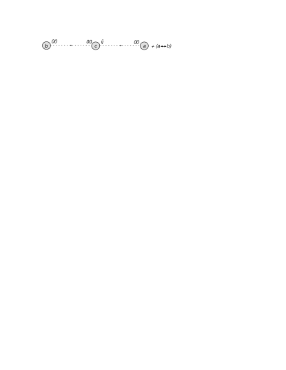
(c) 3 permutations: $a$, $b$, or $c$ in the middle.

(d) 3 permutations: $a$, $b$, or $c$ in the middle.

(e) 6 permutations: $a$, $b$, or $c$ in the middle.

Two choices for remaining two labels.

(f) 3 permutations: $a$, $b$, or $c$ in the middle.

(g) 6 permutations: $a$, $b$, or $c$ in the center. Two choices for remaining two labels.

(h) 3 permutations: $a$, $b$, or $c$ at the two ends.

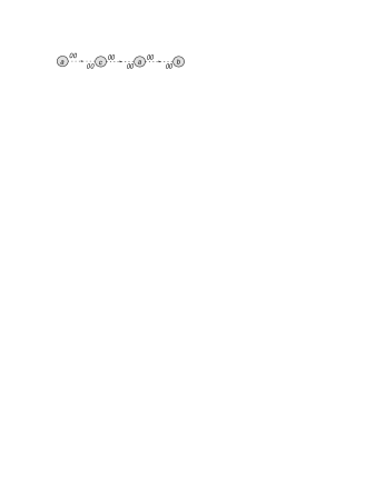
(i) 6 permutations: $a$, $b$, or $c$ for the repeated label. Two choices for remaining two labels.

Figure 10: 2 PN three body diagrams with no graviton vertices.

No graviton vertices  The 3 body diagrams that do not have graviton vertices are:

Fig.(10$$| =i\int{\rm d}t\frac{(d-3)\Gamma\left[\frac{d-3}{2}\right]^{2}}{256(d-2)^{2}\pi^{d-1}}$$a)

$$\qquad\times\frac{M_{a}M_{b}M_{c}}{M_{\text{pl}}^{2(d-2)}R_{ac}^{d-3}R_{bc}^{d-3}}\vec{v}_{a}^{2}$$

Fig.(10$$| =-i\int{\rm d}t\frac{(d-3)\Gamma\left[\frac{d-3}{2}\right]^{2}}{128(d-2)\pi^{d-1}}$$b)

$$\qquad\times\frac{M_{a}M_{b}M_{c}}{M_{\text{pl}}^{2(d-2)}R_{ac}^{d-3}R_{bc}^{d-3}}\vec{v}_{a}\cdot\vec{v}_{c}$$

Fig.(10$$| =i\int{\rm d}t\frac{(d-3)\Gamma\left[\frac{d-3}{2}\right]^{2}}{128(d-2)^{2}\pi^{d-1}}$$c)

$$\qquad\times\frac{M_{a}M_{b}M_{c}}{M_{\text{pl}}^{2(d-2)}R_{ac}^{d-3}R_{bc}^{d-3}}\vec{v}_{c}^{2}$$

Fig.(10$$| =i\int{\rm d}t\frac{3\Gamma\left[\frac{d-1}{2}\right]^{2}}{128(d-2)^{2}\pi^{d-1}}$$d)

$$\qquad\times\frac{M_{a}M_{b}M_{c}}{M_{\text{pl}}^{2(d-2)}R_{ac}^{d-3}R_{bc}^{d-3}}\vec{v}_{c}^{2}$$

Fig.(10$$| =i\int{\rm d}t\frac{\Gamma\left[\frac{d-1}{2}\right]^{2}}{128(d-2)^{2}\pi^{d-1}}$$e)

$$\qquad\times\frac{M_{a}M_{b}M_{c}}{M_{\text{pl}}^{2(d-2)}R_{ac}^{d-3}R_{bc}^{d-3}}\vec{v}_{b}^{2}$$

As with its 2 body counterpart, Fig.(10$|$f) requires some caution when taking the time derivatives. As an example, the integral in the $a-\times-c-b$ diagram, without the constant factors, is

$$\int\text{d}t_{a}\int\text{d}t_{c}\delta[t_{a}-t_{c}]$$

$$\times\bigg{(}\frac{\text{d}|\vec{x}_{c}[t_{c}]-\vec{x}_{b}[t_{c}]|^{3-d}}{\text{d}t_{c}}\frac{\text{d}|\vec{x}_{a}[t_{a}]-\vec{x}_{c}[t_{c}]|^{5-d}}{\text{d}t_{a}}$$

$$+|\vec{x}_{c}[t_{c}]-\vec{x}_{b}[t_{c}]|^{3-d}\frac{\text{d}^{2}|\vec{x}_{a}[t_{a}]-\vec{x}_{c}[t_{c}]|^{5-d}}{\text{d}t_{a}\text{d}t_{c}}\bigg{)}$$

Fig.(10$|$f) is the sum of $a-\times-c-b$ and $b-\times-c-a$, but since differentiation and piecing together the relevant constants are straightforward, we will not display the result.

Fig.(10$$| =i\int{\rm d}t\frac{3\Gamma\left[\frac{d-1}{2}\right]^{3}}{1024(d-2)^{3}\pi^{\frac{3}{2}(d-1)}}$$g)

$$\qquad\times\frac{M_{a}^{2}M_{b}M_{c}}{M_{\text{pl}}^{3(d-2)}R_{ac}^{2(d-3)}R_{bc}^{d-3}}$$

Fig.(10$$| =i\int{\rm d}t\frac{\Gamma\left[\frac{d-1}{2}\right]^{3}}{512(d-2)^{3}\pi^{\frac{3}{2}(d-1)}}$$h)

$$\qquad\times\frac{M_{a}^{2}M_{b}M_{c}}{M_{\text{pl}}^{3(d-2)}R_{ab}^{d-3}R_{ac}^{d-3}R_{bc}^{d-3}}$$

Fig.(10$$| =i\int{\rm d}t\frac{\Gamma\left[\frac{d-1}{2}\right]^{3}}{512(d-2)^{3}\pi^{\frac{3}{2}(d-1)}}$$i)

$$\qquad\times\frac{M_{a}^{2}M_{b}M_{c}}{M_{\text{pl}}^{3(d-2)}R_{ab}^{d-3}R_{ac}^{2(d-3)}}$$

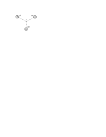
(a) 3 permutations: $a$, $b$, or $c$ carry the $0i$ indices.

(b) No permutations necessary.

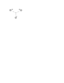
(c) 3 permutations: $a$, $b$, or $c$ carry the $ij$ indices.

(d) 3 permutations: $a$, $b$, or $c$ carry the $00$ indices.

(e) 3 permutations: $a$, $b$, or $c$ carry the $v^{2}$.

Figure 11: 2 PN three body diagrams with graviton vertices: 1 of 2

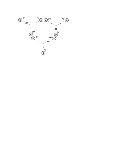
(a) No permutations necessary.

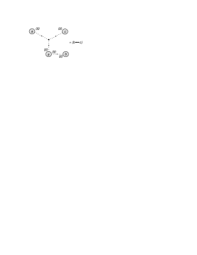
(b) 9 permutations. See text for discussion.

(c) 3 permutations: $a$, $b$, or $c$ for the repeated label.

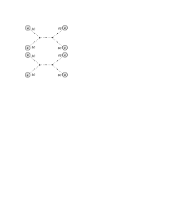
(d) 6 permutations. See text for discussion.

Figure 12: 2 PN three body diagrams with graviton vertices: 2 of 2

Graviton vertices  The rest of the 3 body diagrams contain graviton vertices.

Fig.(11$|$a)  Fig.(11$|$a) requires $I_{0i0000}$ from (III.3.1). For the 3 body case, one sees that $I_{0i0000}$ can be expressed in terms of time- and space-derivatives on $I_{3}$. Specifically,

$$I_{0i0000}[a,b,c]$$

$$=\frac{i}{2(d-2)M_{\text{pl}}^{(d-2)/2}}\int\text{d}t\int\text{d}t_{a}\int\text{d}t_{b}\int\text{d}t_{c}$$

$$\times\delta[t-t_{a}]\delta[t-t_{b}]\delta[t-t_{c}]$$

$$\times\bigg{(}\{\left(2(d-4)v_{a}^{i}\partial_{i}^{b}+(d-5)v_{a}^{i}\partial_{i}^{c}\right)I_{3}[a,b,c]\}$$

$$\quad\times\frac{{\rm d}}{{\rm d}t_{b}}\delta[t_{b}-t]\delta[t_{c}-t]$$

$$+\{\left(2(d-4)v_{a}^{i}\partial_{i}^{c}+(d-5)v_{a}^{i}\partial_{i}^{b}\right)I_{3}[a,b,c]\}$$

$$\quad\times\frac{{\rm d}}{{\rm d}t_{c}}\delta[t_{b}-t]\delta[t_{c}-t]\bigg{)},$$

which means

Fig.(11$$| =\frac{M_{a}M_{b}M_{c}}{4M_{\text{pl}}^{\frac{3}{2}(d-2)}}I_{0i0000}[a,b,c]$$a)

Fig.(11$|$b)  As discussed for Fig.(7$|$a), we have a vanishing diagram when $d=4$ for

Fig.(11$$| \stackrel{{\scriptstyle d=4}}{{=}}0$$b)

Fig.(11$|$c)  The master integral for Fig.(11$|$c) is $I_{ij0000}$ in (III.3.1), whose 3 body expression in terms of $I_{3}$ is

$$I_{ij0000}[a,b,c]$$

$$=i\int\text{d}t\bigg{\{}\frac{\Gamma\left[\frac{d-3}{2}\right]^{2}}{16\pi^{d-1}(d-2)^{2}M_{\text{pl}}^{(d-2)/2}}\vec{v}_{a}^{2}\big{(}R_{ab}^{3-d}R_{ac}^{3-d}$$

$$\qquad-(d-3)\left(R_{ba}^{3-d}R_{bc}^{3-d}+R_{ca}^{3-d}R_{cb}^{3-d}\right)\big{)}$$

$$-\frac{d-3}{2(d-2)M_{\text{pl}}^{(d-2)/2}}v_{a}^{i}v_{a}^{j}$$

$$\qquad\times\left(\partial_{i}^{a}\partial_{j}^{a}+\partial_{i}^{b}\partial_{j}^{b}+\partial_{i}^{c}\partial_{j}^{c}\right)I_{3}[a,b,c]\bigg{\}},$$

so that

Fig.(11$$| =\frac{M_{a}M_{b}M_{c}}{8M_{\text{pl}}^{\frac{3}{2}(d-2)}}I_{ij0000}[a,b,c]$$c)

Fig.(11$|$d)  The 3 body master integral for Fig.(11$|$d) is $I_{0i0j00}$ from (III.3.1), which reads

$$I_{0i0j00}[a,b,c]$$

$$=i\int\text{d}t\bigg{\{}\frac{\Gamma\left[\frac{d-3}{2}\right]^{2}\vec{v}_{a}\cdot\vec{v}_{b}}{64\pi^{d-1}(d-2)M_{\text{pl}}^{(d-2)/2}}$$

$$\times\big{(}(d-4)\left(R_{ab}^{3-d}R_{ac}^{3-d}+R_{ba}^{3-d}R_{bc}^{3-d}\right)$$

$$\qquad+(d-2)R_{ca}^{3-d}R_{cb}^{3-d}\big{)}$$

$$-\frac{1}{2(d-2)M_{\text{pl}}^{(d-2)/2}}v_{a}^{i}v_{b}^{j}$$

$$\qquad\times\big{(}(d-4)\partial_{i}^{b}\partial_{j}^{a}$$

$$\qquad+(d-3)(\partial_{i}^{c}\partial_{j}^{a}+\partial_{i}^{b}\partial_{j}^{c})\big{)}I_{3}[a,b,c]\bigg{\}},$$

leading us to

Fig.(11$$| =\frac{M_{a}M_{b}M_{c}}{2M_{\text{pl}}^{\frac{3}{2}(d-2)}}I_{0i0j00}[a,b,c]$$d)

Fig.(11$|$e)  Fig.(11$|$e) involves products of $\vec{v}^{2}$ with the 1 PN 3-graviton master integral $I_{000000}$.

Fig.(11$$| =\int\text{d}t\frac{M_{a}M_{b}M_{c}}{16M_{\text{pl}}^{\frac{3}{2}(d-2)}}\vec{v}_{c}^{2}I_{000000}[a,b,c]$$e)

$$=-i\int{\rm d}t\frac{(d-3)^{2}\Gamma\left[\frac{d-3}{2}\right]^{2}M_{a}M_{b}M_{c}}{256\pi^{d-1}(d-2)^{2}M_{\text{pl}}^{2(d-2)}}\vec{v}_{c}^{2}$$

$$\times\left(R_{ab}^{3-d}R_{ac}^{3-d}+R_{bc}^{3-d}R_{ac}^{3-d}+R_{ab}^{3-d}R_{bc}^{3-d}\right)$$

Fig.(12$|$a)  The 3 body master integral for Fig.(12$|$a) is $I_{000000\times}$ from (III.3.1):

$$I_{000000\times}[a,b,c]=\widetilde{I}_{\times}[a,b,c]+\widetilde{I}_{\times}[b,a,c]+\widetilde{I}_{\times}[c,b,a]$$

$$\widetilde{I}_{\times}[a,b,c]$$

$$\equiv\frac{i(d-3)^{2}}{(d-2)^{2}M_{\text{pl}}^{(d-2)/2}}\int\text{d}t\int\text{d}t_{a}\int\text{d}t_{b}\int\text{d}t_{c}$$

$$\times\bigg{(}I_{3}[a,b,c]$$

$$\qquad+\frac{\Gamma\left[\frac{d-3}{2}\right]\Gamma\left[\frac{d-5}{2}\right]}{64\pi^{d-1}}\left(R_{ba}^{5-d}R_{bc}^{3-d}+R_{ca}^{5-d}R_{cb}^{3-d}\right)\bigg{)}$$

$$\times\frac{\text{d}^{2}}{\text{d}t_{a}^{2}}\delta[t-t_{a}]\delta[t-t_{b}]\delta[t-t_{c}]$$

In terms of $I_{000000\times}[a,b,c]$,

Fig.(12$$| =\frac{M_{a}M_{b}M_{c}}{8M_{\text{pl}}^{\frac{3}{2}(d-2)}}I_{000000\times}[a,b,c]$$a)

Fig.(12$|$b)  For the class of diagrams represented by Fig.(12$|$b), the 9 permutations include both types of diagrams where the 2 world line sources attached to the 3 graviton vertex not contracted with an additional world line can either belong to the same particle (6 of them) or 2 distinct particles (3 of them). (Fig.(12$|$b) itself belongs to the latter.) We observe, as we did in the 2 body case, that these diagrams are products of the lowest order $\langle h_{00}h_{00}\rangle$ with the 1 PN 3-graviton master integral $I_{000000}$ in (III.2.2).

Fig.(12$$|$$b)

$$=\frac{\Gamma\left[\frac{d-1}{2}\right]M_{a}^{2}M_{b}M_{c}}{64(d-2)\pi^{\frac{d-1}{2}}M_{\text{pl}}^{\frac{5}{2}(d-2)}}\int\text{d}t$$

$$\times\left(R_{ac}^{3-d}I_{000000}[a,b,a]+R_{ab}^{3-d}I_{000000}[a,c,a]\right)$$

$$=-i\int{\rm d}t\frac{(d-3)^{2}\Gamma\left[\frac{d-3}{2}\right]^{2}\Gamma\left[\frac{d-1}{2}\right]M_{a}^{2}M_{b}M_{c}}{1024M_{\text{pl}}^{3(d-2)}\pi^{\frac{3}{2}(d-1)}(d-2)^{3}}$$

$$\quad\times\left(R_{ac}^{3-d}R_{ab}^{2(3-d)}+R_{ac}^{2(3-d)}R_{ab}^{3-d}\right),$$ (39)

For the other 6 permutations where the 2 world line sources attached to the 3 graviton vertex not contracted with an additional world line belong to the same particle, the analog to the above 2 terms in (III.3.2) have different numerical factors in front of them.

Fig.(12$|$c)  Fig.(12$|$c) is a straightforward application of $I_{00000000}$ in (III.3.1) and (B).

Fig.(12$$| =\int\text{d}t\frac{M_{a}^{2}M_{b}M_{c}}{32M_{\text{pl}}^{2(d-2)}}I_{00000000}[a,a,b,c]$$c)

$$=-i\int{\rm d}t\frac{(d-3)(d(7d-51)+86)\Gamma\left[\frac{d-3}{2}\right]^{3}}{8192\pi^{\frac{3}{2}(d-1)}(d-2)^{3}}$$

$$\times\frac{M_{a}^{2}M_{b}M_{c}}{M_{\text{pl}}^{3(d-2)}}\left(R_{bc}^{3-d}R_{ab}^{2(3-d)}+R_{ac}^{2(3-d)}R_{bc}^{3-d}\right)$$

Fig.(12$|$d)  Referring to the discussion under the 2 body counterpart of Fig.(12$|$d), if $a$ is the repeated label for a given 3 body diagram, then the 6 permutations of particle labels are: $2\times(aa|bc)$, $2\times(ab|ac)$, and $2\times(ac|ab)$.

The master integrals for Fig.(12$|$d) can be found in (34,35,36,37). $I_{0000-0000}^{\text{I}}$ is the linear combination of products of (B). As we did in the 2 body case, $I_{0000-0000}^{\text{II}}$ can be done using (B), its derivatives, and derivatives on $I_{3}$. When $a$ is the repeated particle label, $I_{0000-0000}^{\text{II}}$ is

$$I_{0000-0000}^{\text{II}}[a,a,b,c]$$

$$\stackrel{{\scriptstyle d=4}}{{=}}\frac{i}{256M_{\text{pl}}^{2}\pi^{3}}\int\text{d}t\bigg{(}\frac{R_{ab}^{2}-R_{ac}^{2}}{2R_{ac}^{2}R_{bc}^{3}}-\frac{R_{ab}^{2}+R_{ac}^{2}-R_{bc}^{2}}{2R_{ab}^{3}R_{ac}^{2}}$$

$$\quad\qquad-\frac{R_{ab}^{2}+R_{ac}^{2}-R_{bc}^{2}}{2R_{ab}^{2}R_{ac}^{3}}+\frac{R_{ab}-R_{bc}}{R_{ac}^{3}R_{bc}}$$

$$\quad\qquad+\frac{R_{ac}-R_{bc}}{R_{ab}^{3}R_{bc}}+\frac{R_{ac}^{2}-R_{ab}^{2}}{2R_{ab}^{2}R_{bc}^{3}}\bigg{)}$$ (40)

We will leave $I_{0000-0000}^{\text{III}}[q,q,r,s]$ for possible future work.

In terms of the $I_{0000-0000}$ in (34,35,36,37), we have

Fig.(12$$| =\frac{M_{a}^{2}M_{b}M_{c}}{64M_{\text{pl}}^{2(d-2)}}I_{0000-0000}[a,a,b,c]$$d)

III.3.3 4 body diagrams

(a) 4 permutations: $a$, $b$, $c$, or $e$ for the center label.

(b) 6 permutations. See text for discussion.

Figure 13: 2 PN four body diagrams with no graviton vertices

No graviton vertices  The vertex-less diagrams are:

Fig.(13$$| =i\int{\rm d}t\frac{3\Gamma\left[\frac{d-1}{2}\right]^{3}}{512(d-2)^{3}\pi^{\frac{3}{2}(d-1)}}$$a)

$$\quad\times\frac{M_{a}M_{b}M_{c}M_{e}}{M_{\text{pl}}^{3(d-2)}R_{ae}^{d-3}R_{be}^{d-3}R_{ce}^{d-3}}$$

For the class of diagrams in Fig.(13$|$b), there are 12 ways to choose 2 out of the $\{a,b,c,e\}$ for the middle two labels, but there is a reflection symmetry, and hence there are 6 distinct permutations of the particle labels.

Fig.(13$$| =i\int{\rm d}t\frac{\Gamma\left[\frac{d-1}{2}\right]^{3}}{512(d-2)^{3}\pi^{\frac{3}{2}(d-1)}}\frac{M_{a}M_{b}M_{c}M_{e}}{M_{\text{pl}}^{3(d-2)}}$$b)

$$\times\left(R_{ae}^{3-d}R_{bc}^{3-d}R_{ce}^{3-d}+R_{ac}^{3-d}R_{be}^{3-d}R_{ce}^{3-d}\right)$$

(a) 4 permutations. $a,b,c$ or $e$ has 2 graviton fields.

(b) No permutations necessary.

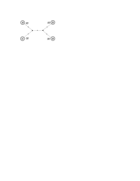
(c) 6 permutations. See text for discussion.

Figure 14: 2 PN four body diagrams with graviton vertices

Graviton vertices  The rest of the 4 body diagrams have graviton vertices.

Fig.(14$|$a)  The class of diagrams in Fig.(14$|$a), like those of its 2- and 3-body counterparts, involve products of the lowest order $\langle h_{00}h_{00}\rangle$ with the 1 PN 3-graviton vertex integral $I_{000000}$. Also, there are 4 distinct permutations, with the world line operator with 2 graviton fields associated with either $a$, $b$, $c$, or $e$.

Fig.(14$$|$$a)

$$=\int\text{d}t\frac{\Gamma\left[\frac{d-1}{2}\right]M_{a}M_{b}M_{c}M_{e}}{64(d-2)M_{\text{pl}}^{\frac{5(d-2)}{2}}\pi^{\frac{d-1}{2}}}$$

$$\times\big{(}R_{ae}^{3-d}I_{000000}[b,c,e]+R_{ce}^{3-d}I_{000000}[a,b,e]$$

$$\qquad+R_{be}^{3-d}I_{000000}[a,c,e]\big{)}$$

$$=-i\int{\rm d}t\frac{(d-3)^{2}\Gamma\left[\frac{d-1}{2}\right]\Gamma\left[\frac{d-3}{2}\right]^{2}M_{a}M_{b}M_{c}M_{e}}{1024\pi^{\frac{3}{2}(d-1)}M_{\text{pl}}^{3(d-2)}(d-2)^{3}}$$

$$\times\bigg{(}\left(R_{bc}^{3-d}R_{be}^{3-d}+R_{ce}^{3-d}R_{be}^{3-d}+R_{bc}^{3-d}R_{ce}^{3-d}\right)R_{ae}^{3-d}$$

$$\qquad+\left(R_{ab}^{3-d}R_{ae}^{3-d}+R_{be}^{3-d}R_{ae}^{3-d}+R_{ab}^{3-d}R_{be}^{3-d}\right)R_{ce}^{3-d}$$

$$\qquad+\left(R_{ac}^{3-d}R_{ae}^{3-d}+R_{ce}^{3-d}R_{ae}^{3-d}+R_{ac}^{3-d}R_{ce}^{3-d}\right)R_{be}^{3-d}\bigg{)}$$

Fig.(14$|$b)  Another straightforward application of $I_{00000000}$ in (III.3.1) and (B) provides us with

Fig.(14$$|$$b)

$$=\int\text{d}t\frac{M_{a}M_{b}M_{c}M_{e}}{16M_{\text{pl}}^{2(d-2)}}I_{00000000}[a,b,c,e]$$

$$=-i\int{\rm d}t\frac{(d-3)(d(7d-51)+86)\Gamma\left[\frac{d-3}{2}\right]^{3}}{4096\pi^{\frac{3}{2}(d-1)}(d-2)^{3}}$$

$$\quad\times\frac{M_{a}M_{b}M_{c}M_{e}}{M_{\text{pl}}^{3(d-2)}}\bigg{(}R_{ab}^{3-d}R_{ac}^{3-d}R_{ae}^{3-d}+R_{be}^{3-d}R_{ce}^{3-d}R_{ae}^{3-d}$$

$$\qquad+R_{ab}^{3-d}R_{bc}^{3-d}R_{be}^{3-d}+R_{ac}^{3-d}R_{bc}^{3-d}R_{ce}^{3-d}\bigg{)}$$

Fig.(14$|$c)  Referring to the discussion under the 2 body counterpart of Fig.(14$|$c), the 6 permutations of particle labels are: $2\times(ab|ce)$, $2\times(ac|be)$, and $2\times(ae|bc)$.

The master integrals for Fig.(14$|$c) can be found in (34,35,36,37). $I_{0000-0000}^{\text{I}}$ is the linear combination of products of (B). As we did in the 2 body case, $I_{0000-0000}^{\text{II}}$ can be done using (B), its derivatives, and derivatives on $I_{3}$. We have given the explicit expression for $I_{0000-0000}^{\text{II}}$ in the 3 body case (III.3.2), but the 4 body one is too lengthy to display.

$I_{0000-0000}^{\text{III}}[q,r,s,u]$ is left for possible future work.

In terms of the $I_{0000-0000}$ in (34,35,36,37), we have

Fig.(14$$| =\frac{M_{a}M_{b}M_{c}M_{e}}{32M_{\text{pl}}^{2(d-2)}}I_{0000-0000}[a,b,c,e]$$c)

III.3.4 $\mathcal{O}[v^{4}]$ Effective Lagrangian

Adding all the relevant diagrams, their permutations and the second order relativistic correction to kinetic energy from the $\eta_{\mu\nu}v^{\mu}v^{\nu}$ in the infinitesimal proper time $\text{d}s$ now gives us the effective lagrangian describing the gravitational dynamics of $n$ point masses at $\mathcal{O}[v^{4}]$ relative to Newtonian gravity in 3+1 dimensions:

$$L^{\text{(2 PN)}}_{\text{eff}} \stackrel{{\scriptstyle d=4}}{{=}}L_{4}^{\text{2 Body}}+L_{4}^{\text{3 Body}}+L_{4}^{\text{4 Body}}$$ (41)

$$L_{4}^{\text{2 Body}} \equiv\frac{1}{2}\sum_{\begin{subarray}{c}1\leq a,b\leq n\\ a\neq b\end{subarray}}\bigg{\{}\frac{M_{a}}{16}\vec{v}_{a}^{6}+\frac{M_{b}}{16}\vec{v}_{b}^{6}$$

$$+\frac{G_{\text{N}}M_{a}M_{b}}{R_{ab}}\bigg{(}\vec{R}_{ab}\cdot\vec{v}_{a}\left(\frac{7}{4}\vec{v}_{a}\cdot\dot{\vec{v}}_{b}-\frac{3}{2}\vec{v}_{b}\cdot\dot{\vec{v}}_{b}\right)+\vec{R}_{ba}\cdot\vec{v}_{b}\left(\frac{7}{4}\vec{v}_{b}\cdot\dot{\vec{v}}_{a}-\frac{3}{2}\vec{v}_{a}\cdot\dot{\vec{v}}_{a}\right)$$

$$\qquad-\frac{1}{8}\left(\frac{\vec{R}_{ab}\cdot\vec{v}_{a}}{R_{ab}}\right)^{2}\left(\vec{R}_{ba}\cdot\dot{\vec{v}}_{b}+\vec{v}_{b}^{2}\right)-\frac{1}{8}\left(\frac{\vec{R}_{ba}\cdot\vec{v}_{b}}{R_{ab}}\right)^{2}\left(\vec{R}_{ab}\cdot\dot{\vec{v}}_{a}+\vec{v}_{a}^{2}\right)$$

$$\qquad+\frac{3}{4}\left(\vec{v}_{a}^{2}+\vec{v}_{b}^{2}-2\ \vec{v}_{a}\cdot\vec{v}_{b}\right)\frac{\vec{R}_{ab}\cdot\vec{v}_{a}}{R_{ab}}\frac{\vec{R}_{ba}\cdot\vec{v}_{b}}{R_{ab}}+\frac{3}{8}\frac{(\vec{R}_{ab}\cdot\vec{v}_{a})^{2}(\vec{R}_{ba}\cdot\vec{v}_{b})^{2}}{R_{ab}^{4}}$$

$$\qquad+\frac{1}{8}\left(\vec{R}_{ba}\cdot\dot{\vec{v}}_{b}\ \vec{v}_{a}^{2}+\vec{R}_{ab}\cdot\dot{\vec{v}}_{a}\ \vec{v}_{b}^{2}\right)+\frac{1}{8}\vec{R}_{ab}\cdot\dot{\vec{v}}_{a}\ \vec{R}_{ba}\cdot\dot{\vec{v}}_{b}$$

$$\qquad+\frac{15}{8}\dot{\vec{v}}_{a}\cdot\dot{\vec{v}}_{b}\ R_{ab}^{2}+\frac{7}{8}(\vec{v}_{a}^{4}+\vec{v}_{b}^{4})+\frac{1}{4}(\vec{v}_{a}\cdot\vec{v}_{b})^{2}+\frac{3}{8}\vec{v}_{a}^{2}\vec{v}_{b}^{2}-\frac{5}{4}(\vec{v}_{a}^{2}+\vec{v}_{b}^{2})\vec{v}_{a}\cdot\vec{v}_{b}\bigg{)}$$

$$+\frac{G_{\text{N}}^{2}M_{a}M_{b}}{R_{ab}^{2}}\bigg{(}-\frac{3}{2}\frac{M_{a}(\vec{R}_{ba}\cdot\vec{v}_{b})^{2}+M_{b}(\vec{R}_{ab}\cdot\vec{v}_{a})^{2}}{R_{ab}^{2}}-2(M_{a}+M_{b})\frac{\vec{R}_{ab}\cdot\vec{v}_{a}\ \vec{R}_{ba}\cdot\vec{v}_{b}}{R_{ab}^{2}}$$

$$\qquad-(2M_{a}+M_{b})\vec{R}_{ab}\cdot\dot{\vec{v}}_{a}-(2M_{b}+M_{a})\vec{R}_{ba}\cdot\dot{\vec{v}}_{b}$$

$$\qquad+\vec{v}_{a}^{2}\left(2M_{a}+\frac{11}{4}M_{b}\right)+\vec{v}_{b}^{2}\left(2M_{b}+\frac{11}{4}M_{a}\right)-\frac{9}{2}\vec{v}_{a}\cdot\vec{v}_{b}\left(M_{a}+M_{b}\right)\bigg{)}$$

$$-\frac{G_{\text{N}}^{3}M_{a}M_{b}}{R_{ab}^{3}}\left(M_{a}M_{b}+\frac{3}{2}(M_{a}^{2}+M_{b}^{2})\right)\bigg{\}}$$ (42)

$$L_{4}^{\text{3 Body}} \equiv\frac{1}{3!}\sum_{\begin{subarray}{c}1\leq a,b,c\leq n\\ a,b,c\text{ distinct}\end{subarray}}\bigg{\{}G_{\text{N}}^{2}M_{a}M_{b}M_{c}$$

$$\qquad\times\bigg{(}\frac{1}{R_{ab}R_{ac}}\left(\frac{9}{2}\vec{v}_{a}^{2}+8\vec{v}_{b}\cdot\vec{v}_{c}\right)+\frac{1}{R_{ab}R_{bc}}\left(\frac{9}{2}\vec{v}_{b}^{2}+8\vec{v}_{a}\cdot\vec{v}_{c}\right)+\frac{1}{R_{ac}R_{bc}}\left(\frac{9}{2}\vec{v}_{c}^{2}+8\vec{v}_{a}\cdot\vec{v}_{b}\right)$$

$$\qquad-\frac{8}{(R_{ab}+R_{ac}+R_{bc})^{2}}\left(\frac{\vec{R}_{ba}\cdot\vec{v}_{b}\vec{R}_{ca}\cdot\vec{v}_{c}}{R_{ab}R_{ac}}+\frac{\vec{R}_{ab}\cdot\vec{v}_{a}\vec{R}_{cb}\cdot\vec{v}_{c}}{R_{ab}R_{bc}}+\frac{\vec{R}_{ac}\cdot\vec{v}_{a}\vec{R}_{bc}\cdot\vec{v}_{b}}{R_{ac}R_{bc}}\right)$$

$$\qquad+\frac{4}{R_{ab}+R_{ac}+R_{bc}}\left(\frac{\vec{v}_{a}^{2}}{R_{bc}}+\frac{\vec{v}_{b}^{2}}{R_{ac}}+\frac{\vec{v}_{c}^{2}}{R_{ab}}\right)$$

$$\qquad+\bigg{[}\frac{1}{2R_{ab}R_{ac}^{3}}\left(\vec{R}_{ac}\cdot\vec{v}_{a}\vec{R}_{ba}\cdot\vec{v}_{b}+\vec{R}_{ac}\cdot\vec{v}_{a}\vec{R}_{ca}\cdot\vec{v}_{c}+\vec{R}_{ba}\cdot\vec{v}_{b}\vec{R}_{ca}\cdot\vec{v}_{c}+2(\vec{R}_{ca}\cdot\vec{v}_{c})^{2}\right)$$

$$\qquad-\frac{1}{R_{ab}R_{ac}}\left(\vec{R}_{ba}\cdot\dot{\vec{v}}_{b}+\frac{7}{2}\vec{v}_{a}\cdot\vec{v}_{b}+\frac{5}{2}\vec{v}_{b}^{2}\right)$$

$$\qquad+\frac{1}{(R_{ab}+R_{ac}+R_{bc})^{2}}\bigg{(}\frac{1}{R_{ab}^{2}}\left(4\vec{R}_{ab}\cdot\vec{v}_{c}\vec{R}_{ba}\cdot\vec{v}_{b}+8\vec{R}_{ab}\cdot\vec{v}_{a}\vec{R}_{ab}\cdot\vec{v}_{c}-2(\vec{R}_{ab}\cdot\vec{v}_{a})^{2}-2(\vec{R}_{ab}\cdot\vec{v}_{c})^{2}\right)$$

$$\qquad\qquad+\frac{1}{R_{ab}R_{ac}}\left(4\vec{R}_{ac}\cdot\vec{v}_{b}\vec{R}_{ba}\cdot\vec{v}_{b}-8\vec{R}_{ac}\cdot\vec{v}_{b}\vec{R}_{ba}\cdot\vec{v}_{c}+12\vec{R}_{ac}\cdot\vec{v}_{a}\vec{R}_{ba}\cdot\vec{v}_{c}-12\vec{R}_{ac}\cdot\vec{v}_{a}\vec{R}_{ba}\cdot\vec{v}_{b}\right)\bigg{)}$$

$$\qquad+\frac{1}{R_{ab}+R_{ac}+R_{bc}}\bigg{(}\frac{1}{R_{ab}^{3}}\left(8\vec{R}_{ab}\cdot\vec{v}_{a}\vec{R}_{ab}\cdot\vec{v}_{c}+4\vec{R}_{ab}\cdot\vec{v}_{c}\vec{R}_{ba}\cdot\vec{v}_{b}-2(\vec{R}_{ab}\cdot\vec{v}_{c})^{2}-2(\vec{R}_{ab}\cdot\vec{v}_{a})^{2}\right)$$

$$\qquad\qquad+\frac{1}{R_{ab}}\left(2\vec{v}_{a}^{2}-4\vec{v}_{a}\cdot\vec{v}_{c}-2\vec{R}_{ab}\cdot\dot{\vec{v}}_{a}\right)\bigg{)}+\text{$5$ other permutations of $\{a,b,c\}$}\bigg{]}\bigg{)}$$

$$+G_{\text{N}}^{3}M_{a}M_{b}M_{c}\bigg{(}\bigg{[}\frac{(M_{a}+M_{c})R_{ab}^{2}}{R_{ac}^{2}R_{bc}^{3}}+\frac{2M_{b}R_{ab}}{R_{ac}R_{bc}^{3}}-\frac{3M_{a}}{R_{ab}^{3}}$$

$$\qquad-\frac{1}{R_{ab}R_{ac}^{2}}\left(M_{a}+\frac{3}{2}M_{c}\right)+\text{$5$ other permutations of $\{a,b,c\}$}\bigg{]}$$

$$\qquad+\frac{1}{16\pi^{2}}\left(M_{a}I_{22}[a,a,b,c]+M_{b}I_{22}[b,b,a,c]+M_{c}I_{22}[c,c,a,b]\right)-2\left(\frac{M_{a}}{R_{bc}^{3}}+\frac{M_{b}}{R_{ac}^{3}}+\frac{M_{c}}{R_{ab}^{3}}\right)\bigg{)}\bigg{\}}$$ (43)

$$L_{4}^{\text{4 Body}} \equiv\frac{1}{4!}\sum_{\begin{subarray}{c}1\leq a,b,c,e\leq n\\ a,b,c,e\text{ distinct}\end{subarray}}G_{\text{N}}^{3}M_{a}M_{b}M_{c}M_{e}$$

$$\qquad\times\bigg{\{}\frac{I_{22}[a,b,c,e]}{8\pi^{2}}-3\left(\frac{1}{R_{ab}R_{ac}R_{ae}}+\frac{1}{R_{ba}R_{bc}R_{be}}+\frac{1}{R_{ca}R_{cb}R_{ce}}+\frac{1}{R_{ea}R_{eb}R_{ec}}\right)$$

$$\qquad\qquad+\bigg{[}\frac{1}{R_{ab}+R_{ac}+R_{bc}}\left(\frac{R_{bc}}{R_{ab}R_{ac}R_{ae}}+\frac{2R_{ae}^{2}}{R_{ab}R_{be}^{3}}-\frac{2R_{ab}}{R_{ae}^{3}}\right)$$

$$\qquad\qquad\qquad+\text{$23$ other permutations of $\{a,b,c,e\}$}\bigg{]}\bigg{\}}$$ (44)

$$I_{22}[q,r,s,u] \equiv\lim_{\begin{subarray}{c}\varepsilon\to 0^{+}\\ \text{after integration}\end{subarray}}\int\text{d}^{3-2\varepsilon}y\int\text{d}^{3-2\varepsilon}z\ \delta^{ij}\delta^{mn}\bigg{(}(\partial_{i}^{q}R_{qy}^{-1+2\varepsilon})(\partial_{m}^{r}R_{ry}^{-1+2\varepsilon})(R_{yz}^{-1+2\varepsilon})(\partial_{j}^{s}R_{sz}^{-1+2\varepsilon})(\partial_{n}^{u}R_{uz}^{-1+2\varepsilon})$$

$$\qquad\qquad\qquad\qquad+(\partial_{i}^{q}R_{qy}^{-1+2\varepsilon})(\partial_{m}^{r}R_{ry}^{-1+2\varepsilon})(R_{yz}^{-1+2\varepsilon})(\partial_{n}^{s}R_{sz}^{-1+2\varepsilon})(\partial_{j}^{u}R_{uz}^{-1+2\varepsilon})\bigg{)}$$

$$\qquad\qquad\qquad\qquad+\text{5 permutations of }\{\vec{x}_{q},\vec{x}_{r},\vec{x}_{s},\vec{x}_{u}\},\qquad R_{qz}\equiv|\vec{x}_{q}-\vec{z}|$$ (45)

The permutations in the definitions of $L_{4}^{\text{3 Body}}$ and $L_{4}^{\text{4 Body}}$ means one would have to take the terms in the given square brackets $[\dots]$, consider the resulting expressions obtained from permuting the particle labels as stated, and sum them all up at the end. For $I_{22}[q,r,s,u]$, if $(qr|su)$ represents the term with $\vec{x}_{q}$ and $\vec{x}_{r}$ occurring in the $\vec{y}$ integration and the $\vec{x}_{s}$ and $\vec{x}_{u}$ in the $\vec{z}$ integration, then the 6 permutations in the definition of $I_{22}$ are: $2\times(qr|su)$, $2\times(qs|ru)$ and $2\times(qu|rs)$.

Relation to L${}_{\text{ADM}}$  As a (partial) check of these results, we shall construct here a coordinate transformation that would bring the 2 body portion of $L^{\text{(2 PN)}}_{\text{eff}}$ into the 2 body, acceleration-independent, lagrangian $L_{\text{ADM}}$ in the literature; for example, eq. (178) of Blanchet Blanchet2BodyLADM . (This construction can be found in Damour and Schäfer DamourSchaeferNBody ; DamourSchaeferRedefinition .) First, we note that defining

$$x^{i}_{a}[t] \equiv z^{i}_{a}[t]+\delta z^{i}_{a}[t],$$

where $\delta z_{a}^{i}$ is assumed to be small relative to $z_{a}^{i}$ (an assumption to be justified shortly), would modify the form of the lagrangian $L[\{x_{a},\vec{v}_{a},\dots\}]$ up to first order in $\delta z$ in the following manner:

$$L[\{\vec{x}_{a}, \vec{v}_{a},\dot{\vec{v}}_{a},\dots\}]$$

$$=L[\{\vec{z}_{a},\dot{\vec{z}}_{a},\ddot{\vec{z}}_{a},\dots\}]+\frac{\delta L}{\delta z}\delta z+\text{total derivative}$$

$$\frac{\delta L}{\delta z}\delta z \equiv\sum_{1\leq a\leq n}\sum_{s=0}^{\infty}\left(\frac{\text{d}^{s}}{\text{d}t^{s}}\frac{\partial L}{\partial(\text{d}^{s}\vec{z}_{a}/\text{d}t^{s})}\right)\cdot\delta\vec{z}_{a}$$

In particular, varying the Newtonian lagrangian $L_{\text{0 PN}}$ gives us

$$\sum_{a}\frac{\delta L_{\text{0 PN}}}{\delta\vec{x}_{a}}\cdot\delta\vec{x}_{a}$$

$$=-\sum_{a\neq b}M_{a}\left(\ddot{\vec{x}}_{a}+\frac{G_{\text{N}}M_{b}}{R_{ab}^{3}}\vec{R}_{ab}\right)\cdot\delta\vec{x}_{a}$$ (46)

Before proceeding with any coordinate transformation, however, one needs to first re-write the terms quadratic in accelerations, $\sum_{i,j;a,b}\ddot{x}_{a}^{i}\ddot{x}_{b}^{j}\tilde{L}^{ij}\subset L^{\text{(2 PN)}}_{\text{eff}}$ as

$$\sum_{1\leq i,j\leq 3}\sum_{1\leq a,b\leq n}\ddot{x}_{a}^{i}\ddot{x}_{b}^{j}\tilde{L}^{ij}$$

$$=\sum_{i,j;a,b}\bigg{\{}\left(\ddot{x}_{a}^{i}+\frac{G_{\text{N}}M_{b}}{R_{ab}^{3}}R_{ab}^{i}\right)\left(\ddot{x}_{b}^{j}+\frac{G_{\text{N}}M_{a}}{R_{ba}^{3}}R_{ba}^{j}\right)\tilde{L}^{ij}$$

$$\quad-\ddot{x}_{a}^{i}\frac{G_{\text{N}}M_{a}}{R_{ba}^{3}}R_{ba}^{j}\tilde{L}^{ij}-\frac{G_{\text{N}}M_{b}}{R_{ba}^{3}}R_{ab}^{i}\ddot{x}_{b}^{j}\tilde{L}^{ij}$$

$$\quad-\frac{G_{\text{N}}M_{b}}{R_{ba}^{3}}R_{ab}^{i}\frac{G_{\text{N}}M_{a}}{R_{ba}^{3}}R_{ba}^{j}\tilde{L}^{ij}\bigg{\}}$$ (47)

Because the term in the first line on the right hand side of (III.3.4) contains the “square” of the Newtonian equations of motion, namely $(1/M_{a})(\delta L_{\text{0 PN}}/\delta z_{a}^{i})(1/M_{b})(\delta L_{\text{0 PN}}/\delta z_{b}^{j})$, and because $(1/M)(\delta L_{\text{0 PN}}/\delta z+\delta L_{\text{1 PN}}/\delta z+\dots)=0$, we see that this first term on the right hand side of (III.3.4) scales as $[(1/M)\delta L_{\text{0 PN}}/\delta z]^{2}\sim[(1/M)\delta L_{\text{1 PN}}/\delta z]^{2}\sim[v^{4}/r]^{2}$ and therefore can be discarded at the 2 PN order.

Removal of accelerations  The reason for linearizing the acceleration dependent terms in $L_{\text{2 PN}}$, keeping only the second and third lines on the right hand side of (III.3.4) is this. Denoting this linearized form of $L_{\text{2 PN}}$ as $L^{\ell}_{\text{2 PN}}$ and referring to the $-M_{a}\ddot{\vec{x}}_{a}\cdot\delta\vec{x}_{a}$ piece in (III.3.4), we see that the remaining acceleration dependent terms in $L^{\ell}_{\text{2 PN}}$ can now be removed by defining

$$\delta\vec{z}_{a}^{\text{(I)}}\equiv\left.\frac{1}{M_{a}}\frac{\partial L^{\ell}_{\text{2 PN}}}{\partial\ddot{\vec{x}}_{a}}\right|_{\vec{x}_{a}=\vec{z}_{a}}$$ (48)

Further transformations  One can perform further coordinate transformations without re-introducing acceleration dependent terms. The key is to make the $-M_{a}\ddot{\vec{x}}_{a}\cdot\delta\vec{x}_{a}$ piece in (III.3.4) part of a total time derivative. Observe that, by having some arbitrary functional $F$ depend only on positions and velocities, we have the identity

$$\sum_{a}\ddot{\vec{x}}_{a}\cdot\frac{\partial F}{\partial\dot{\vec{x}}_{a}}[\{\vec{x}_{a},\dot{\vec{x}}_{a}\}]$$

$$=\frac{\text{d}F}{\text{d}t}[\{\vec{x}_{a},\dot{\vec{x}}_{a}\}]-\sum_{a}\dot{\vec{x}}_{a}\cdot\frac{\partial F}{\partial\vec{x}_{a}}[\{\vec{x}_{a},\dot{\vec{x}}_{a}\}]$$

Therefore, by putting

$$\delta\vec{z}_{a}^{\text{(II)}} \equiv\frac{1}{M_{a}}\frac{\partial F}{\partial\dot{\vec{z}}_{a}}[\{\vec{z}_{b},\dot{\vec{z}}_{b}\}],$$

we can replace $-\sum_{a}M_{a}\ddot{\vec{z}}_{a}\cdot\delta\vec{z}_{a}^{\text{(II)}}=-\sum_{a}\ddot{\vec{z}}_{a}\cdot\partial F/\partial\dot{\vec{z}}_{a}$ with $\sum_{a}\dot{\vec{z}}_{a}\cdot\partial F/\partial\vec{z}_{a}$.

At this point, let us note that the alterations to the form of the lagrangian due to $\delta z$ (48) occurs solely at the 2 PN order: $\delta\vec{z}\sim rv^{4}$. Hence $\delta z$ is indeed small relative to $\vec{z}_{a}$, and it is only necessary to consider $\delta L_{\text{0 PN}}/\delta z$ and not $\delta L_{\text{1 PN}}/\delta z$, $\delta L_{\text{2 PN}}/\delta z$, nor any corrections that are quadratic or higher polynomials of $\delta z$.

Altogether, the 2 body lagrangian after linearizing the accelerations and after the transformation $\vec{x}_{a}\equiv\vec{z}+\delta\vec{z}_{a}^{\text{(I)}}+\delta\vec{z}_{a}^{\text{(II)}}$, less total derivative terms, now reads

$$L[\{\vec{x}_{a},\vec{v}_{a},\dot{\vec{v}}_{a},\dots\}]$$

$$=L_{\text{0 PN}}[\{\vec{z}_{a},\dot{\vec{z}}_{a}\}]+L_{\text{1 PN}}[\{\vec{z}_{a},\dot{\vec{z}}_{a}\}]$$

$$\qquad+L^{\ell}_{\text{2 PN}}[\{\vec{z}_{a},\dot{\vec{z}}_{a},\ddot{\vec{z}}_{a}\}]$$

$$\quad-\left.\sum_{a\neq b}\left(\ddot{\vec{x}}_{a}+\frac{G_{\text{N}}M_{b}}{R_{ab}^{3}}\vec{R}_{ab}\right)\cdot\frac{\partial L^{\ell}_{\text{2 PN}}}{\partial\ddot{\vec{x}}_{a}}\right|_{\vec{x}_{a}=\vec{z}_{a}}$$ (49)

$$\quad+\left.\sum_{a\neq b}\left(\dot{\vec{x}}_{a}\cdot\frac{\partial F}{\partial\vec{x}_{a}}-\frac{G_{\text{N}}M_{b}}{R_{ab}^{3}}\vec{R}_{ab}\cdot\frac{\partial F}{\partial\dot{\vec{x}}_{a}}\right)\right|_{\vec{x}_{a}=\vec{z}_{a}}$$ (50)

It remains to construct $F[\{\vec{x}_{a},\dot{\vec{x}}_{a}\}]$. From $(1/M)(\partial F/\partial\dot{x})=\delta z\sim rv^{4}$, we must have $F\sim Mrv^{5}$. From (50), we also must have $F\propto M_{a}M_{b}/M_{\text{pl}}^{2}\sim G_{\text{N}}M_{a}M_{b}\sim Mrv^{2}$, since all terms in $L^{\text{(2 PN)}}_{\text{eff}}$ need to contain at least one power of the mass of each of the 2 point particles and at least one power of $G_{\text{N}}$ is required because all the terms (less the $M\vec{v}^{6}/16$) in $L^{\text{(2 PN)}}_{\text{eff}}$ are at least linear in $G_{\text{N}}$. To supply the additional $v^{3}$ needed, we have to consider all possible products of the dimensionless scalars built out of terms occurring at 2 PN order, namely, $\{\vec{v}_{a}^{2},\vec{v}_{b}^{2},\vec{v}_{a}\cdot\vec{v}_{b},G_{\text{N}}M_{a}/R_{ab},G_{\text{N}}M_{b}/R_{ab}\}$ for the $v^{2}$ terms and $\{\vec{v}_{a}\cdot\vec{R}_{ab}/R_{ab},\vec{v}_{b}\cdot\vec{R}_{ba}/R_{ab}\}$ for the $v^{1}$ terms. The most general $F$ is thus

$$F[\{\vec{x}_{s},\dot{\vec{x}}_{s}|s=1,2,\dots,n\}]$$

$$=\frac{1}{2}\sum_{a\neq b}\bigg{\{}\frac{G_{\text{N}}^{2}M_{a}M_{b}(c_{1}M_{a}+c_{2}M_{b})}{R_{ab}^{2}}\vec{v}_{a}\cdot\vec{R}_{ab}$$

$$\quad+\frac{G_{\text{N}}M_{a}M_{b}}{R_{ab}}\vec{v}_{a}\cdot\vec{R}_{ab}\bigg{(}c_{3}\vec{v}_{a}^{2}+c_{4}\vec{v}_{b}^{2}+c_{5}\vec{v}_{a}\cdot\vec{v}_{b}$$

$$\qquad+c_{6}\left(\frac{\vec{v}_{a}\cdot\vec{R}_{ab}}{R_{ab}}\right)^{2}+c_{7}\left(\frac{\vec{v}_{b}\cdot\vec{R}_{ba}}{R_{ab}}\right)^{2}$$

$$\qquad+c_{8}\left(\frac{\vec{v}_{a}\cdot\vec{R}_{ab}}{R_{ab}}\right)\left(\frac{\vec{v}_{b}\cdot\vec{R}_{ba}}{R_{ab}}\right)\bigg{)}+(a\leftrightarrow b)\bigg{\}},$$ (51)

where the $\{c_{i}|i=1,2,\dots,8\}$ are arbitrary real numbers, and $(a\leftrightarrow b)$ means one would have to take the terms occurring before it and swap all the particle labels $a\leftrightarrow b$.

Computing (49) and (50) with such a $F$ reveals that one would recover the $L_{\text{ADM}}$ in Blanchet Blanchet2BodyLADM from (III.3.4) for

$$c_{1}=0,\quad c_{2}=-\frac{3}{4},\quad c_{3}=0,\quad c_{4}=\frac{1}{2}$$

$$c_{5}=0,\quad c_{6}=0,\quad c_{7}=-c_{8}$$ ,

where $c_{8}$ can be an arbitrary real number.

IV Summary and Discussion

In this paper we have, following nrgr , used a point mass approximation for the $n$-body in general relativity, allowing us to obtain a lagrangian description at the cost of introducing an infinite number of terms in the action. Because we are seeking the 2 PN effective lagrangian, however, only the minimal terms $\{-M_{a}\int\text{d}s_{a}\}$ are necessary. By examining the physical scales in the problem, we have described how to organize our action (2) and outlined an algorithm that would allow us in principle to generate all the necessary Feynman diagrams up to an arbitrary PN order for a given set of point particle actions (minimal or not); as well as automate the computation process so that as few of the Feynman diagrams as possible are left for human evaluation. This way, the post-Newtonian program can be pursued in an efficient and systematic manner within the framework of perturbative field theory, and the necessary software may be developed to tackle the effective 2 body lagrangian calculation at 4 PN and beyond. In the bulk of this work, we obtained in closed form the conservative portion of the effective lagrangian $L_{\text{eff}}[\{\vec{x}_{a},\vec{v}_{a},\dot{\vec{v}}_{a}\}]$ up to 1 PN for the general case of $n$ point masses in $d\geq 4$ spacetime dimensions and up to 2 PN for 2 point masses in (3+1)-dimensions.

It is apparent that the primary bottleneck of higher post-Newtonian calculations is one of calculus. For the $n$-body problem, it is the analytic evaluation of integrals such as $I_{22}$ (III.3.4) and the $I_{1\dots N}$ (62) for $N\geq 4$. At the same time, it is possible that choosing a different gauge from the one used in (7) and/or a different parametrization of $h_{\mu\nu}$ may help reduce the number of diagrams and the amount of work needed in manipulating the momentum dot products from the tensor contraction of graviton vertices in fourier space. The reduction of diagrams at 2 PN was recently demonstrated in the 2 body case computed by Gilmore and Ross GilmoreRoss . They used the full de Donder gauge $S_{\text{gf}}=\int{\rm d}^{d}x\sqrt{g}g^{\alpha\beta}g^{\mu\nu}g^{\sigma\rho}\Gamma_{\sigma\mu\nu}\Gamma_{\rho\alpha\beta}$ and the Kaluza-Klein parametrization for $h_{\mu\nu}$, first introduced to the PN problem by Kol and Smolkin KolSmolkin . Some other possible choices include the ADM variables normally associated with the (3+1)-decomposition of the spacetime metric. Yet another possibility is to employ the gravitational lagrangian constructed by Bern and Grant BernGrant_EH=YMYM using quantum chromodynamics gluon amplitudes, up to the 5-graviton interaction; this is sufficient, however, only to 3 PN.

We end with a cautionary remark against taking superposition too literally within the post-Newtonian framework. By using the 1 PN lagrangian (III.2.3) in 3 spatial dimensions, and taking the continuum limit, the force $\vec{F}$ experienced by a stationary point mass $M_{x}$ located at $\vec{r}$ away from the center of a static, spherical, hollow shell of surface mass density $\sigma$ and coordinate radius $R$ can be shown to be

$$\vec{F} \equiv M_{x}\frac{\text{d}^{2}\vec{r}}{\text{d}t^{2}}$$

$$=-M_{x}^{2}\frac{\pi RG_{\text{N}}^{2}\sigma}{1+12\pi RG_{\text{N}}\sigma}\frac{\partial}{\partial\vec{r}}\left(\frac{1}{|\vec{r}|}\ln\left|\frac{|\vec{r}|+R}{|\vec{r}|-R}\right|\right),$$

which evidently diverges as the point mass approaches the surface of the shell. Because the force would vanish if gravity were purely Newtonian, such a result for a first order calculation most likely indicates the breakdown of perturbation theory in this regime, since the post-Newtonian lagrangian was derived with an implicit assumption that the point masses involved were well separated, i.e. $r_{\text{s}}\ll r$.

V Acknowledgements

I thank Tanmay Vachaspati for encouraging me to complete this work and for comments on the draft. I would like to thank Luc Blanchet, Alessandra Buonanno and Harsh Mathur for their help and discussions. I also wish to thank Umberto Cannella for bringing to my attention several typographical errors.

Most of the calculations were done using Mathematica mathematica , often in conjunction with the package FeynCalc feyncalc . All Feynman diagrams were drawn with JaxoDraw JaxoDraw . This work was supported in part by the U.S. Department of Energy and FQXi at Case Western Reserve University.

Appendix A The $N$–graviton Feynman Rule

Here we outline an algorithm that can be implemented on symbolic and tensor manipulation software such as Mathematica mathematica and the package FeynCalc feyncalc , to generate the Feynman rule for the $N\geq 2$ graviton vertex in Minkowski space.

Given a product of two function(al)s $f[h]g[h]$ the term that contains exactly $n$ powers of $h$ is a discrete convolution

$$(f\cdot g|n)[h]=\sum_{m=0}^{n}(f|m)[h](g|n-m)[h]$$

where $(A|m)[h]$ denotes the term in $A$ that contains exactly $m$ powers of $h$. Here we also assume that both $f$ and $g$ can be developed as power series expansions starting from the zeroth power in $h$.

With this observation, the term in the Einstein-Hilbert lagrangian containing exactly $n$ powers of the graviton field is given by

$$-2M_{\text{pl}}^{d-2}\sum_{m=0}^{n}\int{\rm d}^{d}x\left(\left.\sqrt{|g|}\right|m\right)\left(R|n-m\right)$$ (52)

where

$$g_{\mu\nu} \equiv\eta_{\mu\nu}+h_{\mu\nu}$$ (53)

$$\left(\left.\sqrt{|g|}\right|n\right) =\frac{1}{n!}\left.\frac{\text{d}^{n}}{\text{d}\epsilon^{n}}\right|_{\epsilon=0}$$

$$\quad\text{exp}\left[\frac{1}{2}\sum_{s=1}^{n}\left\{\frac{(-)^{s+1}\epsilon^{s}}{s}\text{Tr}\left(\eta^{-1}h\right)^{s}\right\}\right]$$

$$\text{Tr}\left(\eta^{-1}h\right)^{s} =h^{\nu_{s}}_{\phantom{\nu_{s}}\nu_{1}}h^{\nu_{1}}_{\phantom{\nu_{1}}\nu_{2}}\dots h^{\nu_{s-1}}_{\phantom{\nu_{s-1}}\nu_{s}}$$

$$(\mathcal{R}|n) =\sum_{m=0}^{n}(g|m)^{\beta\nu}(R|n-m)^{\alpha}_{\phantom{\alpha}\beta\alpha\nu}$$

$$(g|n)^{\alpha\beta} =\left\{\begin{array}[]{ll}\eta^{\alpha\beta}&\text{if $n=0$}\\ (-)^{n}h^{\alpha}_{\phantom{\alpha}\mu_{1}}h^{\mu_{1}}_{\phantom{\alpha}\mu_{2}}\dots h^{\mu_{n-1}\beta}&\text{if $n>0$}\end{array}\right.$$

$$(\Gamma|n)^{\alpha}_{\phantom{\alpha}\mu\nu} =\frac{1}{2}(g|n-1)^{\alpha\lambda}\left(\partial_{\mu}h_{\nu\lambda}+\partial_{\nu}h_{\mu\lambda}-\partial_{\lambda}h_{\mu\nu}\right)$$

$$(R|n)^{\alpha}_{\phantom{\alpha}\beta\mu\nu} =\partial_{\mu}(\Gamma|n)^{\alpha}_{\phantom{\alpha}\beta\nu}-(\mu\leftrightarrow\nu)$$

$$\quad+\sum_{m=0}^{n}(\Gamma|m)^{\alpha}_{\phantom{\alpha}\mu\lambda}(\Gamma|n-m)^{\lambda}_{\phantom{\lambda}\beta\nu}-(\mu\leftrightarrow\nu)$$

Note that the action for GR contains a total $d$-derivative term $-2M_{\text{pl}}^{d-2}\int{\rm d}^{d}x\ \eta^{\mu\nu}\left(\partial_{\alpha}\Gamma^{\alpha}_{\mu\nu}-\partial_{\mu}\Gamma^{\alpha}_{\nu\alpha}\right)$, which needs to be discarded when deriving the Feynman rules. Furthermore, these Feynman rules will also be modified accordingly when a gauge fixing term is added.

Because the graviton field is symmetric in its indices, to obtain the $N$ graviton vertex with external indices $\{\alpha_{1},\beta_{1}\},\dots,\{\alpha_{N},\beta_{N}\}$ given the action (52) containing exactly $N$ powers of the graviton field, we first choose one particular set of contractions between the graviton fields in (52) with the $N$ external ones. We then replace each field $h_{\mu\nu}$ in (52) with the identity tensor $\mathbb{I}^{\alpha_{\ell}\beta_{\ell}}_{\phantom{\alpha_{\ell}\beta_{\ell}}\mu\nu}$ carrying the indices $\{\alpha_{\ell},\beta_{\ell}\}$ that correspond to those on the $\ell$th external field $h^{\text{ext}}_{\alpha_{\ell}\beta_{\ell}}$ it is being contracted with. The identity tensor reads

$$\mathbb{I}^{\alpha_{\ell}\beta_{\ell}}_{\phantom{\alpha_{\ell}\beta_{\ell}}\mu\nu} \equiv\frac{1}{2}\left(\delta^{\alpha_{\ell}}_{\phantom{\alpha_{\ell}}\mu}\delta^{\beta_{\ell}}_{\phantom{\beta_{\ell}}\nu}+\delta^{\alpha_{\ell}}_{\phantom{\alpha_{\ell}}\nu}\delta^{\beta_{\ell}}_{\phantom{\beta_{\ell}}\mu}\right)$$

In momentum $(k-)$space, if we define the direction of momentum to be always flowing into the $N$ graviton vertex, we would also replace partial derivatives occurring in (52) using the prescription

$$\partial_{\lambda}h_{\mu\nu}\to ik_{\lambda_{\ell}}\mathbb{I}^{\alpha_{\ell}\beta_{\ell}}_{\phantom{\alpha_{\ell}\beta_{\ell}}\mu\nu},$$

where $\lambda_{\ell}$ is the $\lambda$th component of the $d$-vector $k$ of the $\ell$th external graviton $h_{\alpha_{\ell}\beta_{\ell}}$ that is contracted with $h_{\mu\nu}$.

The complete Feynman rule for the $N$ graviton vertex would be found by summing up the results from the above procedure for all the $N!$ possible permutations of the external indices. An example featuring the 3-graviton Feynman rule can be found in appendix B of nrgr .

Appendix B Integrals

In this section we review the techniques involved in performing the Feynman integrals encountered in the $n$ body problem at 2 PN.

The starting point is the observation (usually attributed to Schwinger) that one may employ the integral representation of the Gamma function, $\Gamma[z]/b^{z}=\int_{0}^{\infty}t^{z-1}e^{-bt}\text{d}t$, for Re$[b]>0$, to first give us the formula for combining multiple denominators,

$$\frac{1}{A_{1}^{\sigma_{1}}\dots A_{N}^{\sigma_{N}}} =\left(\prod_{s=1}^{N}\frac{1}{\Gamma[\sigma_{s}]}\int_{0}^{1}\text{d}\alpha_{s}\ \alpha_{s}^{\sigma_{s}-1}\right)$$

$$\times\frac{\Gamma\left[\sum_{r=1}^{N}\sigma_{r}\right]\delta\left[1-\sum_{r=1}^{N}\alpha_{r}\right]}{\left(\sum_{r=1}^{N}\alpha_{r}A_{r}\right)^{\sigma_{1}+\dots+\sigma_{N}}},$$ (55)

and second, together with the gaussian integral $\int\exp[-x^{2}]\text{d}x=\pi^{1/2}$, to further yield

$$\int\frac{\text{d}^{\lambda}z}{(\vec{z}^{2}+\Delta)^{\sigma}} =\frac{\pi^{\lambda/2}\Gamma\left[\sigma-\frac{\lambda}{2}\right]}{\Gamma[\sigma]\Delta^{\sigma-\frac{\lambda}{2}}},$$ (56)

and

$$\int\frac{\text{d}^{\lambda}p}{(2\pi)^{\lambda}}\frac{e^{i\vec{p}\cdot\vec{x}}}{[\vec{p}^{2}]^{\sigma}} =\frac{\Gamma\left[\frac{\lambda}{2}-\sigma\right]}{4^{\sigma}\pi^{\lambda/2}\Gamma[\sigma]|\vec{x}|^{\lambda-2\sigma}}, \vec{x}\neq\vec{0}$$ for

$$=0, \text{for $\vec{x}=\vec{0}$},$$ (57)

where the second equality is to be understood within the framework of dimensional regularization.

An important corollary of (B) and (56) is

$$\int\frac{\text{d}^{\lambda}z}{[\vec{z}^{2}]^{\sigma_{1}}[(\vec{z}-\vec{x})^{2}]^{\sigma_{2}}}$$

$$=\frac{\pi^{\lambda/2}\Gamma[\frac{\lambda}{2}-\sigma_{1}]\Gamma[\frac{\lambda}{2}-\sigma_{2}]\Gamma[\sigma_{1}+\sigma_{2}-\frac{\lambda}{2}]}{\Gamma[\sigma_{1}]\Gamma[\sigma_{2}]\Gamma[\lambda-\sigma_{1}-\sigma_{2}][\vec{x}^{2}]^{\sigma_{1}+\sigma_{2}-\frac{\lambda}{2}}}.$$ (58)

By considering single and double spatial derivatives of (B), we may also obtain the formulas:

$$\int{\rm d}^{\lambda}z\frac{(x-z)^{i}}{|\vec{z}|^{\rho_{1}}|\vec{x}-\vec{z}|^{\rho_{2}}}$$ (59)

$$=\frac{\pi^{\lambda/2}\Gamma\left[\frac{\lambda-\rho_{1}}{2}\right]\Gamma\left[\frac{\lambda-\rho_{2}+2}{2}\right]\Gamma\left[\frac{\rho_{1}+\rho_{2}-\lambda}{2}\right]}{\Gamma\left[\frac{\rho_{1}}{2}\right]\Gamma\left[\frac{\rho_{2}}{2}\right]\Gamma\left[\lambda-\frac{\rho_{1}+\rho_{2}-2}{2}\right]}\frac{x^{i}}{|\vec{x}|^{\rho_{1}+\rho_{2}-\lambda}}$$

$$\int{\rm d}^{\lambda}z\frac{(x-z)^{i}(x-z)^{j}}{|\vec{z}|^{\tau_{1}}|\vec{x}-\vec{z}|^{\tau_{2}}}$$ (60)

$$=\frac{\pi^{\lambda/2}\Gamma\left[\frac{\lambda-\tau_{1}}{2}\right]\Gamma\left[\frac{\tau_{1}+\tau_{2}-2-\lambda}{2}\right]\Gamma\left[\frac{\lambda-\tau_{2}+2}{2}\right]}{2\Gamma\left[\frac{\tau_{1}}{2}\right]\Gamma\left[\frac{\tau_{2}}{2}\right]\Gamma\left[\lambda-\frac{\tau_{1}+\tau_{2}-2}{2}\right](2(\lambda+1)-(\tau_{1}+\tau_{2}))}$$

$$\times\bigg{(}(\lambda-\tau_{2}+2)(\tau_{1}+\tau_{2}-2-\lambda)\frac{x^{i}x^{j}}{|\vec{x}|^{\tau_{1}+\tau_{2}-\lambda}}$$

$$\qquad+\delta^{ij}\frac{\lambda-\tau_{1}}{|\vec{x}|^{\tau_{1}+\tau_{2}-2-\lambda}}\bigg{)}$$

$$\int{\rm d}^{\lambda}z\frac{(x_{a}-z)^{i}(x_{b}-z)^{j}}{|\vec{z}-\vec{x}_{a}|^{\rho_{a}}|\vec{z}-\vec{x}_{b}|^{\rho_{b}}}$$ (61)

$$=\frac{\pi^{\lambda/2}\Gamma\left[\frac{\lambda-\rho_{a}+2}{2}\right]\Gamma\left[\frac{\lambda-\rho_{b}+2}{2}\right]\Gamma\left[\frac{\rho_{a}-2+\rho_{b}-\lambda}{2}\right]}{2\Gamma\left[\frac{\rho_{a}}{2}\right]\Gamma\left[\frac{\rho_{b}}{2}\right]\Gamma\left[\lambda-\frac{\rho_{a}+\rho_{b}-4}{2}\right]}$$

$$\times\bigg{(}\frac{\delta^{ij}}{|\vec{x}_{b}-\vec{x}_{a}|^{\rho_{a}+\rho_{b}-2-\lambda}}$$

$$\qquad-\left(\rho_{a}+\rho_{b}-\lambda-2\right)\frac{(x_{a}-x_{b})^{i}(x_{a}-x_{b})^{j}}{|\vec{x}_{b}-\vec{x}_{a}|^{\rho_{a}+\rho_{b}-\lambda}}\bigg{)}$$

The last formula (61) has been derived from (B) by re-defining $\vec{x}\equiv\vec{x}_{a}-\vec{x}_{b}$ and shifting integration variables before performing the appropriate derivatives.

N point integrals  We next review the evaluation of the “$N$-point” integrals first carried out by Boos and Davydychev BoosDavydychev3NointMasslessVertexType ; DavydychevNPointMasslessVertexType .

$$I_{1\dots N}\equiv\int_{\mathbb{R}^{\lambda}}\frac{\text{d}^{\lambda}z}{\prod_{s=1}^{N}|(\vec{x}_{s}-\vec{z})^{2}|^{\rho_{s}}}.$$ (62)

These integrals can be viewed as the higher $N$ generalizations of the $N=2$ case in (B).

Applying (B) transforms it into

$$I_{1\dots N} =\int_{\mathbb{R}^{\lambda}}\text{d}^{\lambda}z\left(\prod_{s=1}^{N}\frac{1}{\Gamma[\rho_{s}]}\int_{0}^{1}\text{d}\alpha_{s}\ \alpha_{s}^{\rho_{s}-1}\right)$$

$$\times\frac{\Gamma[\rho_{1}+\dots+\rho_{N}]\delta\left[1-\sum_{r=1}^{N}\alpha_{r}\right]}{\left(\vec{z}^{2}+\sum_{r,s=1}^{N}\left(\alpha_{r}\alpha_{s}\vec{x}_{s}^{2}-\alpha_{r}\alpha_{s}\vec{x}_{r}\cdot\vec{x}_{s}\right)\right)^{\rho_{1}+\dots+\rho_{N}}},$$

where the constraint $\sum_{r}\alpha_{r}=1$ as well as a shift in the variable $\vec{z}$ have been employed. Writing

$$\sum_{r,s=1}^{N}\left(\alpha_{r}\alpha_{s}\vec{x}_{s}^{2}-\alpha_{r}\alpha_{s}\vec{x}_{r}\cdot\vec{x}_{s}\right) =\frac{1}{2}\sum_{r,s=1}^{N}\alpha_{r}R_{rs}^{2}\alpha_{s},$$

$$R_{rs} \equiv|\vec{x}_{r}-\vec{x}_{s}|$$

and recalling (56) then allow us to deduce

$$I_{1\dots N} =\pi^{\lambda/2}\frac{\Gamma\left[\sum_{r}\rho_{r}-\frac{\lambda}{2}\right]}{\prod_{r}\Gamma[\rho_{r}]}\left(\prod_{s=1}^{N}\int_{0}^{\infty}\text{d}\alpha_{s}\alpha_{s}^{\rho_{s}-1}\right)$$

$$\quad\times\frac{\delta[1-\sum_{r}\alpha_{r}]}{[\frac{1}{2}\sum_{p}\sum_{q}\alpha_{p}\alpha_{q}R_{pq}^{2}]^{\sum_{r}\rho_{r}-\frac{\lambda}{2}}}$$ (63)

By viewing $\alpha_{p}R_{pq}\alpha_{q}$ as components of a $N\times N$ symmetric matrix with zeros on the diagonal, one notes that there are $N(N-1)/2$ distinct terms in the sum in the denominator of (B). To make further progress, one needs to iterate $(L-2)$ times the Mellin-Barnes (MB) integral representation

$$\frac{1}{(X+Y)^{\tau}} =\frac{1}{\Gamma[\tau]}\frac{1}{2\pi i}\int_{-i\infty}^{i\infty}\text{d}s\ \Gamma[s+\tau]\Gamma[-s]\frac{Y^{s}}{X^{s+\tau}},$$

to obtain the $(L-1)$-fold MB representation for the sum of $L$ terms in a denominator raised to some power,

$$\frac{1}{[\sum_{a=1}^{L}u_{a}]^{\tau}} =\frac{1}{\Gamma[\tau]u_{L}^{\tau}}\frac{1}{(2\pi i)^{L-1}}$$

$$\times\left(\prod_{a=1}^{L-1}\int_{-i\infty}^{i\infty}\text{d}s_{a}\Gamma[-s_{a}]\left(\frac{u_{a}}{u_{L}}\right)^{s_{a}}\right)$$

$$\times\Gamma\left[s_{1}+s_{2}+\dots+s_{L-1}+\tau\right]$$ (64)

In these integrals, the contour for the $i$th variable $s_{i}$ is chosen such that the poles of the Gamma functions of the form $\Gamma[\dots-s_{i}]$ lie to the right and those of the Gamma functions of the form $\Gamma[\dots+s_{i}]$ lie to the left.

Using (B) on (B), followed by (B) with $A_{1}=A_{2}=\dots=A_{N(N-1)/2}=1$ and some careful algebraic reasoning, one arrives at the final form of the MB representation for the $N$-point integral,

$$\int_{\mathbb{R}^{\lambda}}\frac{\text{d}^{\lambda}z}{\prod_{s=1}^{N}|(\vec{z}-\vec{x}_{s})^{2}|^{\rho_{s}}} =\frac{\pi^{\lambda/2}[R^{2}_{i^{\prime}j^{\prime}}]^{\frac{\lambda}{2}-\sum_{r}\rho_{r}}}{\Gamma[\lambda-\sum_{r}\rho_{r}]\prod_{r=1}^{N}\Gamma[\rho_{r}]}\frac{1}{(2\pi i)^{(N/2)(N-1)-1}}\prod_{\begin{subarray}{c}\{i,j\}\in\text{upper $\Delta$}\\ \text{of $N\times N$ matrix}\\ \{i,j\}\neq\{i^{\prime},j^{\prime}\}\end{subarray}}^{(N/2)(N-1)-1}\left(\int_{-i\infty}^{i\infty}\text{d}s_{ij}\Gamma[-s_{ij}]\left(\frac{R^{2}_{ij}}{R^{2}_{i^{\prime}j^{\prime}}}\right)^{s_{ij}}\right)$$

$$\times\Gamma\left[\sum_{\begin{subarray}{c}\{k,l\}\in\text{upper $\Delta$}\\ \{k,l\}\neq\{i^{\prime},j^{\prime}\}\end{subarray}}^{(N/2)(N-1)-1}s_{kl}+\sum_{r=1}^{N}\rho_{r}-\frac{\lambda}{2}\right]\prod_{\begin{subarray}{c}1\leq s\leq N\\ s\neq i^{\prime};s\neq j^{\prime}\end{subarray}}\Gamma\left[\rho_{s}+\sum_{\begin{subarray}{c}\{j,k\}\in s^{\rm th}\ \text{row and }s^{\rm th}\ \rm{column}\\ \text{upper }\Delta\end{subarray}}s_{jk}\right]$$

$$\times\Gamma\left[\frac{\lambda}{2}-\sum_{r=1}^{N}\rho_{r}+\rho_{i^{\prime}}-\sum_{\begin{subarray}{c}\{k,l\}\in\text{upper }\Delta\\ k\neq i^{\prime};l\neq i^{\prime}\end{subarray}}s_{kl}\right]\Gamma\left[\frac{\lambda}{2}-\sum_{r=1}^{N}\rho_{r}+\rho_{j^{\prime}}-\sum_{\begin{subarray}{c}\{k,l\}\in\text{upper }\Delta\\ k\neq j^{\prime};l\neq j^{\prime}\end{subarray}}s_{kl}\right]$$ (65)

Here, $\{i^{\prime},j^{\prime}\}$ is some fixed pair of numbers chosen from the “upper triangular” portion of the $N\times N$ matrix of number pairs corresponding to their coordinates on the matrix; namely, the first row on the “upper $\Delta$” reads from left to right, $\{1,2\},\{1,3\},\dots,\{1,N\}$, the second reads $\{2,3\},\{2,4\},\dots,\{2,N\}$, and so on until the $(N-1)$th row, which has only one element, $\{N-1,N\}$.

N = 3  The MB integrals for the $N=3$ case have been explicitly evaluated by Boos and Davydychev BoosDavydychev3NointMasslessVertexType . One has from (B),

$$I_{123} =\frac{\pi^{\lambda/2}[R_{23}^{2}]^{\frac{\lambda}{2}-\sum_{r}\rho_{r}}}{\Gamma[\lambda-\sum_{r}\rho_{r}]\prod_{r}\Gamma[\rho_{r}]}\frac{1}{(2\pi i)^{2}}\int_{-i\infty}^{i\infty}\text{d}u\int_{-i\infty}^{i\infty}\text{d}v\Gamma[-u]\Gamma[-v]\left(\frac{R^{2}_{12}}{R_{23}^{2}}\right)^{u}\left(\frac{R^{2}_{13}}{R_{23}^{2}}\right)^{v}$$

$$\times\Gamma\left[u+v+\sum_{r}\rho_{r}-\frac{\lambda}{2}\right]\Gamma\left[\rho_{1}+u+v\right]\Gamma\left[\frac{\lambda}{2}-\rho_{1}-\rho_{3}-v\right]\Gamma\left[\frac{\lambda}{2}-\rho_{1}-\rho_{2}-u\right]$$ (66)

Assuming there exists a series representation of the integral $I_{123}$ in powers of $R_{12}$ and $R_{13}$, we close the $u$- and $v$-contours on the right, turning each integral into an infinite sum over its residues by noting that $\Gamma[-z]$ has singularities on the complex $z$ plane only in the form of simple poles at zero and the positive integers. (Whether one should close the contour to the left or to the right really depends on the numerical range of $R_{12}$ and $R_{13}$ considered. For instance, the MB representation $(1+z)^{-\lambda}=(2\pi i\Gamma[\lambda])^{-1}\int_{-i\infty}^{+i\infty}\text{d}u\Gamma[u+\lambda]\Gamma[-u]z^{u}$ can be converted into a power series in $1/z$ or $z$, for $\lambda>0$, by closing the contour to the left or right, depending on whether $|z|>1$ or $|z|<1$. Here we will simply assume, for each choice (left or right), there is some region of $R_{12},R_{13}\in\mathbb{R}$ in which it is valid.) The residues of $\Gamma[-z]$ at these locations are

$$\left.{\rm Res}\ \Gamma[-z]\right|_{z=m}=\frac{(-)^{m}}{m!},\quad m=0,+1,+2,\dots$$

Because there are 2 Gamma functions of the form $\Gamma[\dots-u]$ and 2 of the form $\Gamma[\dots-v]$, this converts the 2-fold MB integrals into a 2-fold infinite sum of 4 terms. One can proceed to change summation variables and manipulate the Gamma functions in the summands using the definitions for the Gauss hypergeometric function and the Pochhammer symbol

$${}_{2}F_{1}[a,b;c;z] =\sum_{u=0}^{\infty}\frac{(a)_{u}(b)_{u}}{u!(c)_{u}}z^{u}$$

$$(a)_{u} \equiv a(a+1)\dots(a+(u-1))=\frac{\Gamma[a+u]}{\Gamma[a]}$$

and the relation

$$\Gamma[\tau-m] =\frac{(-)^{m}\Gamma[\tau]}{(1-\tau)_{m}},\ m\in\mathbb{Z},\tau\in\mathbb{C}$$

to further reduce the 2-fold sum into a single sum:

$$I_{abc}[\rho_{a},\rho_{b},\rho_{c}] \equiv\int\frac{\text{d}^{\lambda}z}{[(\vec{z}-\vec{x}_{a})^{2}]^{\rho_{a}}[(\vec{z}-\vec{x}_{b})^{2}]^{\rho_{b}}[(\vec{z}-\vec{x}_{c})^{2}]^{\rho_{c}}}$$

$$=\frac{\pi^{\lambda/2}}{\Gamma[\lambda-\sum_{r}\rho_{r}]\prod_{r}\Gamma[\rho_{r}]}$$

$$\times\sum_{\ell=0}^{\infty}\bigg{\{}[R_{bc}^{2}]^{\frac{\lambda}{2}-\sum_{r}\rho_{r}}\frac{1}{\ell!}\left(\frac{R_{ab}^{2}}{R_{bc}^{2}}\right)^{\ell}\Gamma\left[\frac{\lambda}{2}-\rho_{a}-\rho_{b}\right]\Gamma\left[\frac{\lambda}{2}-\rho_{a}-\rho_{c}\right]\Gamma\left[\sum_{r}\rho_{r}-\frac{\lambda}{2}\right]\Gamma\left[\rho_{a}\right]$$

$$\qquad\times\frac{\left(\sum_{r}\rho_{r}-\frac{\lambda}{2}\right)_{\ell}\left(\rho_{a}\right)_{\ell}}{\left(1-\frac{\lambda}{2}+\rho_{a}+\rho_{b}\right)_{\ell}}\ _{2}F_{1}\left[-\ell,\frac{\lambda}{2}-\rho_{a}-\rho_{b}-\ell;1-\frac{\lambda}{2}+\rho_{a}+\rho_{c};\frac{R_{ac}^{2}}{R_{ab}^{2}}\right]$$

$$+[R_{bc}^{2}]^{-\rho_{c}}\left[R_{ab}^{2}\right]^{\frac{\lambda}{2}-\rho_{a}-\rho_{b}}\frac{1}{\ell!}\left(\frac{R_{ab}^{2}}{R_{bc}^{2}}\right)^{\ell}\Gamma\left[\rho_{a}+\rho_{b}-\frac{\lambda}{2}\right]\Gamma\left[\frac{\lambda}{2}-\rho_{a}-\rho_{c}\right]\Gamma\left[\rho_{c}\right]\Gamma\left[\frac{\lambda}{2}-\rho_{b}\right]$$

$$\qquad\times\frac{\left(\rho_{c}\right)_{\ell}\left(\frac{\lambda}{2}-\rho_{b}\right)_{\ell}}{(1+\frac{\lambda}{2}-\rho_{a}-\rho_{b})_{\ell}}\ _{2}F_{1}\left[-\ell,\rho_{a}+\rho_{b}-\frac{\lambda}{2}-\ell;1-\frac{\lambda}{2}+\rho_{a}+\rho_{c};\frac{R_{ac}^{2}}{R_{ab}^{2}}\right]$$

$$+[R_{bc}^{2}]^{-\rho_{b}}\left[R_{ac}^{2}\right]^{\frac{\lambda}{2}-\rho_{a}-\rho_{c}}\frac{1}{\ell!}\left(\frac{R_{ab}^{2}}{R_{bc}^{2}}\right)^{\ell}\Gamma\left[\frac{\lambda}{2}-\rho_{a}-\rho_{b}\right]\Gamma\left[-\frac{\lambda}{2}+\rho_{a}+\rho_{c}\right]\Gamma\left[\rho_{b}\right]\Gamma\left[\frac{\lambda}{2}-\rho_{c}\right]$$

$$\qquad\times\frac{\left(\rho_{b}\right)_{\ell}\left(\frac{\lambda}{2}-\rho_{c}\right)_{\ell}}{(1-\frac{\lambda}{2}+\rho_{a}+\rho_{b})_{\ell}}\ _{2}F_{1}\left[-\ell,\frac{\lambda}{2}-\rho_{a}-\rho_{b}-\ell;1+\frac{\lambda}{2}-\rho_{a}-\rho_{c};\frac{R_{ac}^{2}}{R_{ab}^{2}}\right]$$

$$+[R_{bc}^{2}]^{\rho_{a}-\frac{\lambda}{2}}\left[R_{ab}^{2}\right]^{\frac{\lambda}{2}-\rho_{a}-\rho_{b}}\left[R_{ac}^{2}\right]^{\frac{\lambda}{2}-\rho_{a}-\rho_{c}}\frac{1}{\ell!}\left(\frac{R_{ab}^{2}}{R_{bc}^{2}}\right)^{\ell}$$

$$\qquad\times\Gamma\left[-\frac{\lambda}{2}+\rho_{a}+\rho_{b}\right]\Gamma\left[-\frac{\lambda}{2}+\rho_{a}+\rho_{c}\right]\Gamma\left[\frac{\lambda}{2}-\rho_{a}\right]\Gamma\left[\lambda-\sum_{r}\rho_{r}\right]$$

$$\qquad\times\frac{\left(\frac{\lambda}{2}-\rho_{a}\right)_{\ell}\left(\lambda-\sum_{r}\rho_{r}\right)_{\ell}}{(1+\frac{\lambda}{2}-\rho_{a}-\rho_{b})_{\ell}}\ _{2}F_{1}\left[-\ell,-\frac{\lambda}{2}+\rho_{a}+\rho_{b}-\ell;1+\frac{\lambda}{2}-\rho_{a}-\rho_{c};\frac{R_{ac}^{2}}{R_{ab}^{2}}\right]\bigg{\}}$$ (67)

As described in Boos and Davydychev BoosDavydychev3NointMasslessVertexType , this sum has a closed form expression in terms of the Appell hypergeometric function $F_{4}$ of two variables, which has a perturbative definition of the form

$$F_{4}\left[\alpha,\beta;\gamma,\delta;x,y\right] =\sum_{m=0}^{\infty}\sum_{n=0}^{\infty}\frac{(\alpha)_{m+n}(\beta)_{m+n}}{(\gamma)_{m}(\delta)_{n}}\frac{x^{m}}{m!}\frac{y^{n}}{n!}.$$

Through the relation

$$\sum_{j=0}^{\infty}\frac{x^{j}}{j!}\frac{(\alpha)_{j}(\beta)_{j}}{(\gamma)_{j}} \ {}_{2}F_{1}\left[-j,1-\gamma-j;\delta;y\right]$$

$$=F_{4}\left[\alpha,\beta;\gamma,\delta;x,xy\right],$$

we now have

$$I_{abc}[\rho_{a},\rho_{b},\rho_{c}] \equiv\int\frac{\text{d}^{\lambda}z}{[(\vec{z}-\vec{x}_{a})^{2}]^{\rho_{a}}[(\vec{z}-\vec{x}_{b})^{2}]^{\rho_{b}}[(\vec{z}-\vec{x}_{c})^{2}]^{\rho_{c}}}$$

$$=\frac{\pi^{\lambda/2}}{\Gamma[\lambda-\sum_{r}\rho_{r}]\prod_{r}\Gamma[\rho_{r}]}$$

$$\times\bigg{\{}[R_{bc}^{2}]^{\frac{\lambda}{2}-\sum_{r}\rho_{r}}\Gamma\left[\frac{\lambda}{2}-\rho_{a}-\rho_{b}\right]\Gamma\left[\frac{\lambda}{2}-\rho_{a}-\rho_{c}\right]\Gamma\left[\sum_{r}\rho_{r}-\frac{\lambda}{2}\right]\Gamma\left[\rho_{a}\right]$$

$$\qquad\times F_{4}\left[\sum_{r}\rho_{r}-\frac{\lambda}{2},\rho_{a};1-\frac{\lambda}{2}+\rho_{a}+\rho_{b},1-\frac{\lambda}{2}+\rho_{a}+\rho_{c};\frac{R_{ab}^{2}}{R_{bc}^{2}},\frac{R_{ac}^{2}}{R_{bc}^{2}}\right]$$

$$+[R_{bc}^{2}]^{-\rho_{c}}\left[R_{ab}^{2}\right]^{\frac{\lambda}{2}-\rho_{a}-\rho_{b}}\Gamma\left[\rho_{a}+\rho_{b}-\frac{\lambda}{2}\right]\Gamma\left[\frac{\lambda}{2}-\rho_{a}-\rho_{c}\right]\Gamma\left[\rho_{c}\right]\Gamma\left[\frac{\lambda}{2}-\rho_{b}\right]$$

$$\qquad\times F_{4}\left[\rho_{c},\frac{\lambda}{2}-\rho_{b};1+\frac{\lambda}{2}-\rho_{a}-\rho_{b},1-\frac{\lambda}{2}+\rho_{a}+\rho_{c};\frac{R_{ab}^{2}}{R_{bc}^{2}},\frac{R_{ac}^{2}}{R_{bc}^{2}}\right]$$

$$+[R_{bc}^{2}]^{-\rho_{b}}\left[R_{ac}^{2}\right]^{\frac{\lambda}{2}-\rho_{a}-\rho_{c}}\Gamma\left[\frac{\lambda}{2}-\rho_{a}-\rho_{b}\right]\Gamma\left[-\frac{\lambda}{2}+\rho_{a}+\rho_{c}\right]\Gamma\left[\rho_{b}\right]\Gamma\left[\frac{\lambda}{2}-\rho_{c}\right]$$

$$\qquad\times F_{4}\left[\rho_{b},\frac{\lambda}{2}-\rho_{c};1-\frac{\lambda}{2}+\rho_{a}+\rho_{b},1+\frac{\lambda}{2}-\rho_{a}-\rho_{c};\frac{R_{ab}^{2}}{R_{bc}^{2}},\frac{R_{ac}^{2}}{R_{bc}^{2}}\right]$$

$$+[R_{bc}^{2}]^{\rho_{a}-\frac{\lambda}{2}}\left[R_{ab}^{2}\right]^{\frac{\lambda}{2}-\rho_{a}-\rho_{b}}\left[R_{ac}^{2}\right]^{\frac{\lambda}{2}-\rho_{a}-\rho_{c}}\Gamma\left[-\frac{\lambda}{2}+\rho_{a}+\rho_{b}\right]\Gamma\left[-\frac{\lambda}{2}+\rho_{a}+\rho_{c}\right]\Gamma\left[\frac{\lambda}{2}-\rho_{a}\right]\Gamma\left[\lambda-\sum_{r}\rho_{r}\right]$$

$$\qquad\times F_{4}\left[\frac{\lambda}{2}-\rho_{a},\lambda-\sum_{r}\rho_{r};1+\frac{\lambda}{2}-\rho_{a}-\rho_{b},1+\frac{\lambda}{2}-\rho_{a}-\rho_{c};\frac{R_{ab}^{2}}{R_{bc}^{2}},\frac{R_{ac}^{2}}{R_{bc}^{2}}\right]\bigg{\}}$$

However, $F_{4}$ is not defined in Mathematica mathematica , whereas the sum in (B) can easily be entered. In particular, at 2 PN, the $n$ body problem requires the knowledge of

$$I_{3}[a,b,c]=\left(\frac{\Gamma\left[\frac{d-3}{2}\right]}{4\pi^{\frac{d-1}{2}}}\right)^{3}I_{123}\left[\rho_{1}=\rho_{2}=\rho_{3}=\frac{d-3}{2}\right].$$

Applying, in $3-2\varepsilon$ spatial dimensions, the Laurent expansion for the Gamma function about negative integers or zero,

$$\Gamma[-m+\varepsilon] =\frac{(-)^{m}}{m!}\left(\frac{1}{\varepsilon}-\gamma_{\rm E}+\sum_{r=1}^{m}\frac{1}{r}+\mathcal{O}[\varepsilon]\right),$$

$$m =0,1,2,\dots,$$

to the summand in (B), before employing the Mathematica command FullSimplify on the summation (B), yields the final form for $I_{3}[a,b,c]$,

$$I_{3}[a,b,c]$$

$$=\frac{1}{64\pi^{2}}\bigg{(}-\frac{1}{\varepsilon}+2-2\gamma_{\rm E}-2\ln[\pi]$$

$$\qquad-4\ln\left|R_{ab}+R_{ac}+R_{bc}\right|+\mathcal{O}[\varepsilon]\bigg{)}$$ (68)

where $\gamma_{\text{E}}=0.57721\dots$ is the Euler-Mascheroni constant and the hyperbolic function identity $\tanh^{-1}[z]=(1/2)(\ln|1+z|-\ln|1-z|)$ was used. An alternate derivation of this result can be found in Blanchet et al. BlanchetEtalIntegral .

A direct computation would show that this result is consistent with the Poisson equation obeyed by the $N=3$ integral in 3 spatial dimensions,

$$\delta^{ij}\partial_{i}^{a}\partial_{j}^{a}I_{123}\left[\rho_{a}=\rho_{b}=\rho_{c}=1/2\right]=-4\pi(R_{ab}R_{ac})^{-1}.$$

Appendix C 3 PN Diagrams

In this section, we collect the fully distinct Feynman diagrams necessary for the computation of the effective lagrangian for $n$ non-rotating, structure-less point masses as described by the minimal action in (2) at the 3 PN order. Fully distinct here means that, to obtain the full 3 PN lagrangian one would have to, whenever applicable:

• Consider all possible permutations of the particle labels of the diagrams displayed.

• For the $n=3,4$ and $5$ diagrams, consider all possible ways of setting some of the particle labels equal to each other, so that from the $n=3$ diagrams one would obtain their $n=2$ counterparts; from the $n=4$ their $n=2$ and $3$ counterparts; and from the $n=5$ their $n=2,3$ and $4$ counterparts.

The 2 body diagrams are in Fig. (15). The 3 body diagrams with graviton vertices are Fig. (16, 17); and those with no graviton vertices are Fig. (18). The 4 body diagrams with graviton vertices are Fig. (19, 20, 21); and those without graviton vertices are Fig. (22, 23). Finally the 5 body diagrams with graviton vertices can be found in Fig. (25), whereas those with none can be found in Fig. (24).

Figure 15: 3 PN 2 body diagrams.

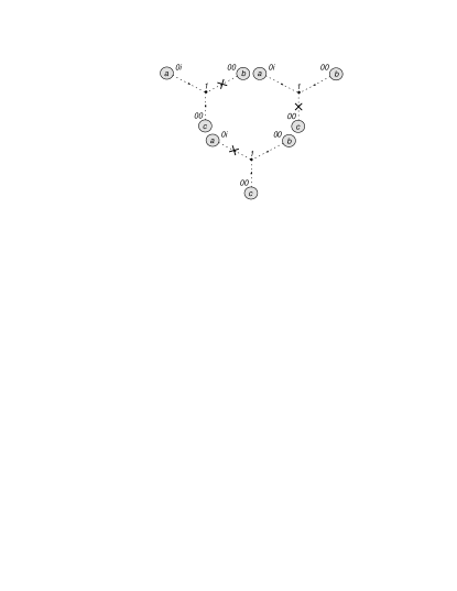
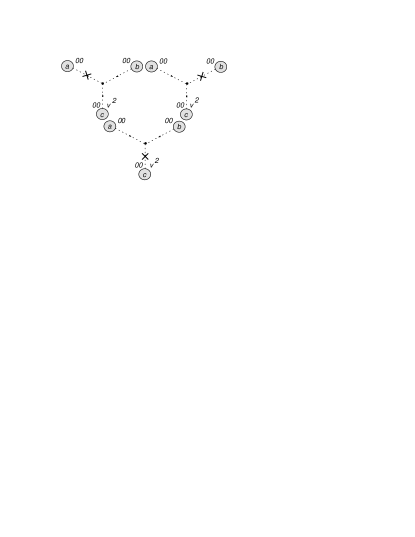
Figure 16: 3 PN 3 body diagrams containing 3 graviton vertices, 1 of 2.

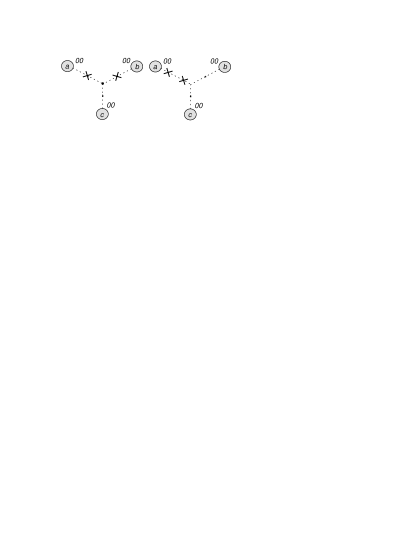
Figure 17: 3 PN 3 body diagrams containing 3 graviton vertices, 2 of 2.

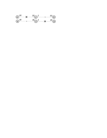
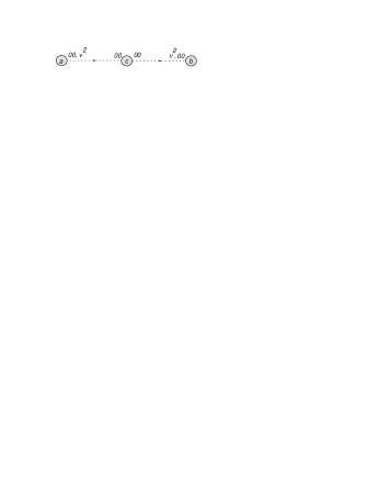
Figure 18: 3 PN 3 body diagrams with no graviton vertices.

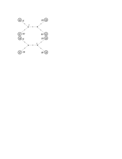
Figure 19: 3 PN 4 body diagrams with graviton vertices, 1 of 3.

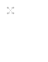
Figure 20: 3 PN 4 body diagrams with graviton vertices, 2 of 3.

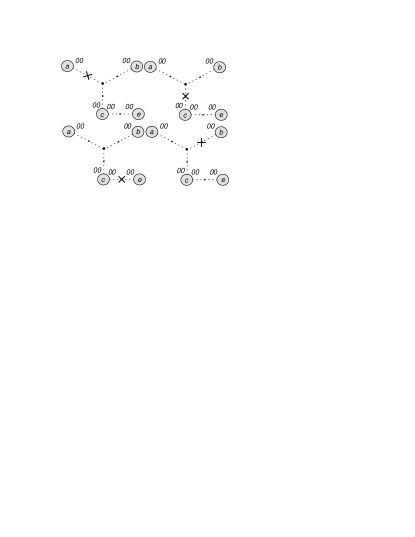
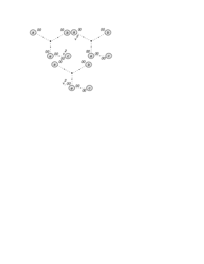
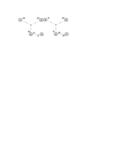
Figure 21: 3 PN 4 body diagrams with graviton vertices, 3 of 3.

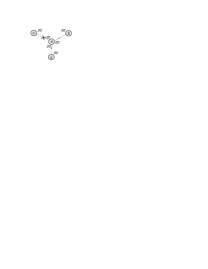
Figure 22: 3 PN 4 body diagrams with no graviton vertices, 1 of 2.

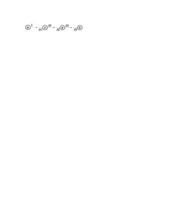
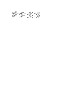
Figure 23: 3 PN 4 body diagrams with no graviton vertices, 2 of 2.

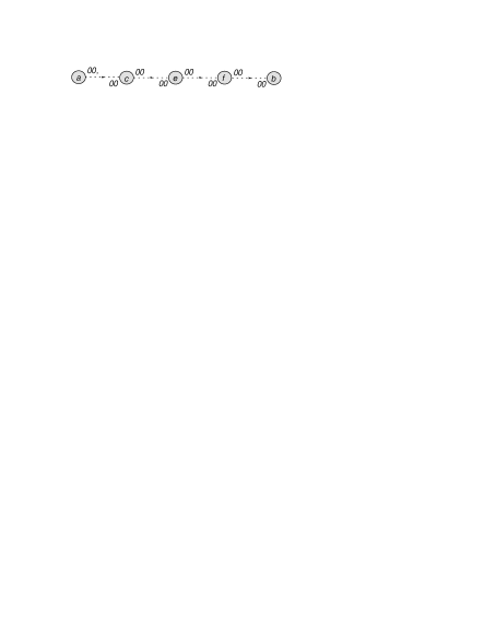
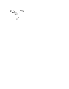
Figure 24: 3 PN 5 body diagrams with no graviton vertices.

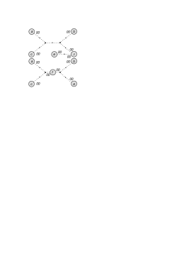
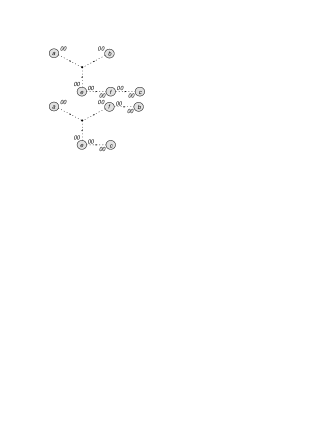
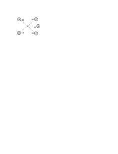
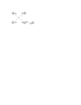
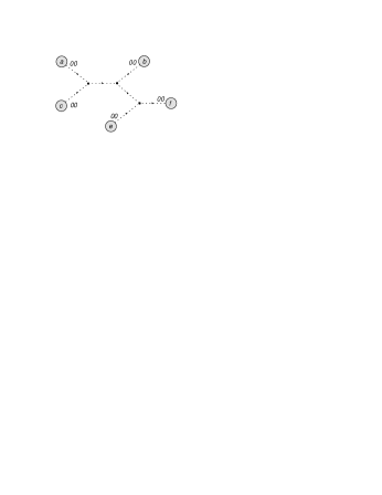
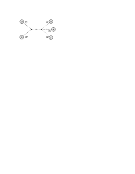
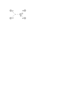
Figure 25: 3 PN 5 body diagrams with graviton vertices.

References

- (1) A. Einstein, L. Infeld and B. Hoffmann, Annals Math. 39, 65 (1938).
- (2) Ohta T., Okamura H., Kimura T., and Hiida K. (1974), Prog Theor Phys 51 1220
- (3) T. Damour and G. Schäfer, Gen. Rel. Grav. 17 (1985) 879
- (4) G. Schäfer, Phys. Lett. A 123, 336 (1987).
- (5) T. Damour and G. Esposito-Farese, Phys. Rev. D 53, 5541 (1996) [arXiv:gr-qc/9506063].
- (6) L. Blanchet, Living Rev. Rel. 5, 3 (2002) [arXiv:gr-qc/0202016].
- (7) D. C. Dai, R. Matsuo and G. Starkman, arXiv:0811.1565 [astro-ph].
- (8) S. G. Turyshev, Annu. Rev. Nucl. Part. Sci. 58, 207 (2008) arXiv:0806.1731 [gr-qc].
- (9) E. E. Boos and A. I. Davydychev, Theor. Math. Phys. 89, 1052 (1991) [Teor. Mat. Fiz. 89, 56 (1991)]. (Available online at: http://wino.physik.uni-mainz.de/~davyd/pubs.html)
- (10) A. I. Davydychev, J. Math. Phys. 32, 1052 (1991).
- (11) L. Blanchet, T. Damour and G. Esposito-Farese, Phys. Rev. D 69, 124007 (2004) [arXiv:gr-qc/0311052].
- (12) V. A. Smirnov, Springer Tracts Mod. Phys. 211, 1 (2004).
- (13) W. D. Goldberger and I. Z. Rothstein, Phys. Rev. D 73, 104029 (2006) [arXiv:hep-th/0409156].
- (14) J. B. Gilmore and A. Ross, Phys. Rev. D 78, 124021 (2008) [arXiv:0810.1328 [gr-qc]].
- (15) V. Cardoso, O. J. C. Dias and P. Figueras, Phys. Rev. D 78, 105010 (2008) [arXiv:0807.2261 [hep-th]].
- (16) T. Damour and G. Schaefer, J. Math. Phys. 32, 127 (1991).
- (17) E. Poisson, arXiv:gr-qc/9912045.
- (18) B. Kol and M. Smolkin, Phys. Rev. D 77, 064033 (2008) [arXiv:0712.2822 [hep-th]].
- (19) Z. Bern and A. K. Grant, Phys. Lett. B 457, 23 (1999) [arXiv:hep-th/9904026].
- (20) Wolfram Research, Inc., Mathematica, Version 5.2, Champaign, IL (2005)
- (21) R. Mertig, M. Boehm and A. Denner, Comp. Phys. Comm. 64 (1991) 345, http://www.feyncalc.org/
- (22) D. Binosi and L. Theussl, Comput. Phys. Commun. 161, 76 (2004) [arXiv:hep-ph/0309015]. http://jaxodraw.sourceforge.net/
- (23) http://www.stargazing.net/yizen/PN.html