Parameters of Herbig Ae/Be and Vega-type stars

Abstract

Context. This work presents the characterization of 27 young early-type stars, most of them in the age range 1–10 Myr, and three –suspected– hot companions of post-T Tauri stars belonging to the Lindroos binary sample. Most of these objects show IR excesses in their spectral energy distributions, which are indicative of the presence of disks. The work is relevant in the fields of stellar physics, physics of disks and formation of planetary systems.

Aims. The aim of the work is the determination of the effective temperature, gravity, metallicity, mass, luminosity and age of these stars. An accurate modelling of their disks needs, as a previous step, the knowledge of most of these parameters, since they will determine the energy input received by the disk and hence, its geometry and global properties.

Methods. Spectral energy distributions and mid-resolution spectra were used to estimate $T_{\rm eff}$, the effective temperature. The comparison of the profiles of the Balmer lines with synthetic profiles provides the value of the stellar gravity, $g_{*}$. High-resolution optical observations and synthetic spectra are used to estimate the metallicity, [M/H]. Once $T_{\rm eff}$, $g_{*}$ and [M/H] are known for each star, evolutionary tracks and isochrones provide estimations of the mass, luminosity, age and distances (or upper limits in some cases). The method is original in the sense that it is distance-independent, i.e. the estimation of the stellar parameters does not require, as it happens in other works, the knowledge of the distance to the object.

Results. Stellar parameters (effective temperature, gravity, metallicity, mass, luminosity, age and distances –or upper limits) are obtained for the sample of stars mentioned above. A detailed discussion on some individual objects, in particular VV Ser, RR Tau, 49 Cet and the three suspected hot companions of post-T Tauris, is presented.

Conclusions. These results, apart from their intrinsic interest, would be extremely valuable to proceed a step further and attempt to model the disks surrounding the stars. The paper also shows the difficulty posed by the morphology and behaviour of the system star+disk in the computation of the stellar parameters.

1 Introduction

One of the most active research areas in PMS (pre-main sequence) stellar physics is the study of stars with protoplanetary disks. Today it is widely accepted that circumstellar disks are a common feature of the star formation processes (Beckwith, 1996). The percentage of the presence of accretion disks around young stars ranges from 50 to 100%, at least for the youngest star-forming regions (Kenyon & Hartmann, 1995; Hillenbrand et al. 1998). A study in the near infrared of young clusters by Haisch et al. (2001) in the age range 0.3–30 Myr shows that at the early ages, the cluster disk fraction is around 80%, and decreases as the cluster age increases, the typical overall disk lifetime being $5-7$ Myr. The work by those authors, confirmed by Hillenbrand (2005), Cieza (2008) and Hernández et al. (2008) was based on samples containing mostly T Tauri stars (spectral types K and M). In the mass range of the Herbig Ae/Be stars (spectral types B to F), Hernández et al. (2005) found that the lifetime of primordial disks is less than $\sim\!3$ Myr. There is evidence that the typical times for disk dissipation depend on stellar mass (e.g. Sicilia-Aguilar et al. 2005), although in all cases this phenomenon seems to occur in the first few million years of the stellar lifetime.

The formation of planets and planetary systems takes place in circumstellar disks. The report in 1995 of the discovery of the first extrasolar planet around a solar-type star, namely 51 Peg, by Mayor & Queloz (1995), and the subsequent detections of candidate planets increased even further the interest in that area, and in particular, the study of the evolution of PMS stars and their disks in a range of ages of the order of $\sim\!10^{6}$ years, when the disks have their characteristic morphology and processes of potential formation of planetesimals have already been triggered.

The mass, radius and effective temperature of the central star will determine the energy received by the disk and therefore –at least in part– its geometry, energy balance, accretion rate and contribution to the spectral energy distribution (SED hereafter). The metal abundance of the star, a parameter which is many times overlooked and assumed to take the solar value, is also an important factor because the gas contained in the disk will have, in a first approximation, a similar metal content, which, in turn, will have an influence on its evolution and the potential formation of planets (see e.g. Wyatt et al. 2007, and references therein). In addition, the gas dominates the mass and dynamics of the disk (e.g. Hillenbrand, 2008). The knowledge of the metallicity is also important to place the star in the appropriate set of evolutionary tracks to determine parameters such as mass, luminosity and age (Merín et al., 2004). Therefore, in this context, the determination of parameters and properties of stars –i.e. what we call their ‘characterization’– in the critical age range of 1–10 Myr, is a necessary step to model accurately the disks.

Several works have aimed at a systematic determination of parameters of PMS and young MS stars (T Tauri, Herbig Ae/Be, Vega and A-shell) with disks. Dunkin et al. (1997a,b) carried out a complete study of 14 Vega-type objects based on high-resolution spectroscopy. Kovalchuk & Pugach (1997) determined the gravity for a sample of 19 Herbig Ae/Be stars. The spectral classification, projected rotational velocities and variability of 80 PMS and young MS stars were studied by Eiroa et al. (2001), Eiroa et al. (2002), Mora et al. (2001) and Oudmaijer et al. (2001). Hernández et al. (2004) carried out an analysis of 75 Herbig Ae/Be stars, deriving spectral types and studying the properties of the extinction caused by the environment of these objects. Acke & Waelkens (2004) presented an abundance study of 24 Herbig Ae/Be and Vega-type stars searching for the $\lambda$ Bootis phenomenon, and Guimarães et al. (2006) determined stellar gravities and metal abundances for 12 Herbig Ae/Be stars. Manoj et al. (2006) studied the evolution of the emission line activity for a sample of 45 Herbig Ae/Be stars and estimated masses, luminosities and ages for an enlarged sample of 91 objects of this type.

In this paper we present the results of the determination of effective temperatures, stellar gravities, metallicities, masses, luminosities, ages and distances for 30 young stars. In Sections 2 and 3 we describe the sample of stars and the observations. Section 4 describes how the stellar parameters have been estimated. Sections 5 and 6 present the results and a detailed discussion. Finally, some remarks are drafted in Section 7.

2 The sample of stars

In this work we study the properties of a sample of 30 early-type objects, namely 19 Herbig Ae/Be (hereafter HAeBe), five Vega-type, three A-shell and three suspected hot companions of post-T Tauri stars (see subsection 6.4 to see why we add the qualifier ‘suspected’ to these stars). In Table 1 we list some properties of the stars. Column 1 gives the identification of the object, column 2 provides other identifications, when available, from the MWC, BD or HD catalogues; column 3, the type of star; column 4, the projected rotational velocity $v\sin i$ and column 5 indicates whether the star has emission in the H$\alpha$ line or not. Since the presence or absence of this emission is an indicator of activity, these data will be useful to discuss the evolutionary status of the objects. The stars have been chosen from the EXPORT sample (Eiroa et al. 2000).

Table 1: The sample of stars.

Star	Other ID	Type of star	$v\sin i$ (km/s)	H$\alpha$
HD 31648	MWC 480	HAeBe	102 $\pm$ 5	Y
HD 58647	BD$-13$ 2008	HAeBe	118 $\pm$ 4	Y
HD 150193	MWC 863	HAeBe		Y
HD 163296	MWC 275	HAeBe	133 $\pm$ 6	Y
HD 179218	MWC 614	HAeBe		Y
HD 190073	MWC 325	HAeBe		Y
HR 10	HD 256	Ash	294 $\pm$ 9	N
HR 26 A	HD 560 A	HPTT		N
HR 2174	HD 4211	Vega	252 $\pm$ 7	N
HR 4757 A	HD 108767 A	HPTT	239 $\pm$ 7	N
HR 5422 A	HD 127304 A	HPTT	7.4 $\pm$ 0.3	N
HR 9043	HD 223884	Vega	205 $\pm$ 18	N
AS 442		HAeBe		Y
BD+31 643	HD 281159	Vega	162 $\pm$ 13	N
$\lambda$ Boo	HD 125162	Vega	129 $\pm$ 7	N
VX Cas		HAeBe	179 $\pm$ 18	Y
SV Cep	BD+72 1031	HAeBe	206 $\pm$ 13	Y
49 Cet	HD 9672	Vega	186 $\pm$ 4	N
24 CVn	HD 118232	Ash	173 $\pm$ 4	N
51 Oph	HD 158643	HAeBe	256 $\pm$ 11	Y
T Ori	BD$-05$ 1329	HAeBe	175 $\pm$ 14	Y
BF Ori	BD$-06$ 1259	HAeBe	37 $\pm$ 2	Y
UX Ori	HD 293782	HAeBe	215 $\pm$ 15	Y
V346 Ori	HD 287841	HAeBe		Y
V350 Ori		HAeBe		Y
XY Per	HD 275877	HAeBe	217 $\pm$ 13	Y
VV Ser		HAeBe	229 $\pm$ 9	Y
17 Sex	HD 88195	Ash	259 $\pm$ 13	N
RR Tau	BD+26 887a	HAeBe	225 $\pm$ 35	Y
WW Vul	HD 344361	HAeBe	220 $\pm$ 22	Y

Notes to Table 1: The abbreviations in column 3 mean: HAeBe (Herbig Ae/Be), HPTT (hot companion of a post-T Tauri star) and Ash (A-shell star).

The data for $v\sin i$ are from Mora et al. (2001). Slight refinements to the results for SV Cep (225 km/s), XY Per (200 km/s) and WW Vul (210 km/s) were presented by Mora et al. (2004). A blank in column 4 means that the star was not observed in high resolution, furthermore the determination of this parameter was not feasible and its value has not been found elsewhere.

Apart from the intrinsic interest of the objects, one of the peculiarities of analysing this kind of early-type objects is that the determination of gravities, as we will see in subsection 4.2, is feasible due to the fact that, for stars with $T_{\rm eff}$ above approximately 7500 K, the shapes of the profiles of the Balmer lines have a strong dependence with the stellar gravity. Provided that an estimation of $T_{\rm eff}$ is available, $\log g_{*}$ can be derived and then proceed with the determination of other stellar parameters.

The stars HR 26 A, HR 4757 A and HR 5422 A, are the hot components of three binary systems whose cool star is a post-T Tauri object. The systems belong to the so-called Lindroos binary sample (Lindroos, 1985). We will discuss their evolutionary status and their physical link with the corresponding cool stars in Section 6.4.

3 The observations

Two sets of observations have been used in this work. Intermediate resolution, high signal-to-noise spectra in the range 3700–6200 Å, were obtained for all the stars with CAFOS (Calar Alto Faint Object Spectrograph) on the 2.2-m telescope at Calar Alto Observatory (CAHA, Almería, Spain). The observations were taken in two campaigns, 28 October–2 November 2004 and 1–4 April 2005. The motivation was to obtain high quality Balmer line profiles, in particular H$\beta$, H$\gamma$ and H$\delta$, in order to estimate the stellar gravities (see subsection 4.2). CAFOS was equipped with a CCD SITe detector of 2048$\times$2048 pixels (pixel size 24 $\mu$m) and the grism Blue-100, centered at 4238 Å, giving a linear dispersion of $\sim 88$ Å/mm (2 Å/pixel), which is equivalent to a resolving power of $\sim\!2500$. A slit width of 130 $\mu$m was used, corresponding to 1.5 arcsec projected on the sky. The usual bias, dark and dome flat-field frames were taken each night. Standard procedures were used to process the data. The nominal positions of the Balmer lines were used to self-calibrate the spectra in wavelength; a second-order polynomial wavelength-pixel was used. The widths of the lines of the calibration Hg-He-Rb lamps were used to obtain the width of the instrumental profile of the spectrograph for each night.

Figure 1: A flow chart sketching the procedure we use to estimate the stellar parameters.

High-resolution echelle spectra were used in the computation of the metallicities (subsection 4.3). These spectra were taken during the four EXPORT campaigns in 1998 and 1999 with the Utrech Echelle Spectrograph (UES) on the 4.2-m William Herschel Telescope (WHT) at the Observatorio del Roque de los Muchachos (La Palma, Spain). UES was set up to provide a wavelength coverage between 3800 and 5900 Å. The spectra were dispersed into 59 echelle orders with a resolving power of 48 000. The slit width was set to 1.15 arcsec projected on the sky. Details on the observing runs and the reduction of the UES observations can be found in Mora et al. (2001).

4 The computation of the stellar parameters

Fig. 1 shows a sketch of the whole procedure we follow to compute the stellar parameters. In the next paragraphs of this Section we describe in detail every step.

4.1 The effective temperature

The effective temperature is the first quantity needed to start the computation of the whole set of parameters. The procedure to estimate $T_{\rm eff}$ followed in this work and also by Merín (2004), consists in a comparison of the observed spectral energy distribution, more precisely of its photospheric part (see subsection 6.1 for a discussion on this), with a grid of low-resolution synthetic spectra (Kurucz, 1993), with different effective temperatures and reddened with a range of extinctions, typically from $E(B\!-\!V)=0.1$ to 1.2, in those cases when no solution with the original models was found. The total-to-selective extinction $R_{V}$ used is 3.1 although some studies (e.g. Hernández et al. 2004) suggest that a higher value ($R_{V}\!\sim\!5$) could be more appropriate to model the extinction caused by the environment of HAeBe stars. We will discuss this choice in subsection 6.4. The synthetic spectra were normalized to the observed SED and the best fits were chosen after a careful comparison and assessment of each case.

In some cases a degeneracy appeared, i.e. two or more synthetic spectra fit reasonably well the observed SED, therefore additional information (e.g. the best fit between the observed and synthetic Balmer profiles) had to be used to break it and choose the correct solution. In subsection 6.4 we show how to solve this and other problems found at this very first step for some of the objects, in particular the very complex cases of VV Ser and RR Tau. The degeneracy cannot be broken using the intrinsic photometric colours of standard stars compared with those of the target stars: two synthetic spectra corresponding to two different sets of values ($T_{\rm eff}$, $g_{*}$) can fit the observed photometric points for two different values of $E(B\!-\!V)$, both of them being consistent with the intrinsic colours of stars of each spectral type reddened to match the observed colours.

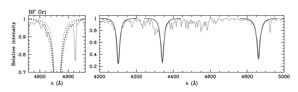
Figure 2: Left: H$\beta$ profile of BF Ori (grey solid line) and synthetic profiles (black dotted lines) computed with $T_{\rm eff}=8970$ K, the effective temperature of this star, and $\log g_{*}=$3.5, 4.0 and 4.5 (the latter profile is the broadest). Right: Spectrum of BF Ori obtained with CAFOS on the 2.2-m telescope at CAHA (grey solid line) and the synthetic profiles for H$\delta$, H$\gamma$ and H$\beta$ computed for $T_{\rm eff}=8970$ K and $\log g_{*}=3.83$ (black solid lines) broadened with the instrumental profile. All the synthetic models shown in this figure were computed with [M/H]=+0.20, which is the metallicity estimated for this star.

The SEDs are built from simultaneous optical and near-infrared (near-IR) photometry obtained in 1998 and 1999 (Eiroa et al. 2001; Oudmaijer et al. 2001). Simultaneity of the observations is a key point at this step, since for highly variable objects, the use of photometry from different epochs could lead to wrong results. Among our data, the photometry corresponding to the maximum of the stellar brightness, i.e. obtained when the star is likely to be less obscured, is used in building the SED. We work here under the hypothesis that the obscuration is caused by the disk, and hence, that the brightest set of magnitudes in the optical and near-IR –up to the wavelength where the thermal emission from the disk starts– represents the stellar photosphere.

Some stars were observed in the range 1200–3200 Å by the International Ultraviolet Explorer (IUE) space observatory; these observations are used with caution to complete the SEDs, due to the variable nature of most of the objects, the non-simultaneity with the optical and near-IR observations. In addition to the method outlined in the first paragraph of this subsection, the comparison between the unreddened synthetic spectra and the ultraviolet part of the SED is particularly useful to have a better estimation of the extinction. AAVSO magnitudes, when they had been measured almost simultaneously with the IUE observations, are used to place at the same level the ultraviolet and the optical/near-IR parts of the SED.

Table 2 gives the results for the effective temperatures found in this work and adopted throughout. In a few cases, specified at the table, values of the effective temperature from other sources have been used. A typical upper limit of the uncertainty in the determination of this parameter is of the order of $\pm 200$ K.

4.2 Stellar gravities

Stellar gravities are estimated by comparing the wings of the Balmer lines H$\beta$, H$\gamma$ and H$\delta$ with synthetic profiles extracted from Kurucz (1993) model atmospheres. The gravity is obtained by measuring the wavelengths of the intensity levels $I\!=\!0.80$ and $I\!=\!0.90$ –the latter only if the profile is clean enough– below the normalized continuum on the blue and red sides of the observed Balmer profiles. These intensities were chosen to avoid potential uncertainties in the overall shape of the wings near the continuum arising both from the normalization of the original spectra and from the presence of weak absorption lines in this region.

A pair of values, namely $\lambda$(blue) and $\lambda$(red), is obtained for each line for the intensity levels mentioned above. Each wavelength is then compared with the corresponding one measured on a grid of synthetic profiles computed for the effective temperature of the star, and different gravities. The initial metallicity adopted is [M/H]=0.0, i.e. solar. The synthetic profiles are convolved with the instrumental response function of the corresponding night. The effect of rotational broadening, even for values of $v\sin i$ as high as $\sim\!250$ km/s, is negligible in the upper part (above $I\!\simeq\!0.50$) of the synthetic Balmer profiles, therefore this broadening was not applied. Linear interpolation was used to convert the discrete grid of wavelengths from the Kurucz models into a continuous functions of $\log g_{*}$. The final result for $\log g_{*}$ is the mean value of the results for each line with an uncertainty corresponding to the standard deviation $\sigma$. The observed Balmer profiles showing emission or strange features due to the presence of several components of different widths were not used for the computations of gravities.

In Fig. 2 we see an example of the determination of the stellar gravity. The panel on the left shows the H$\beta$ line profile (solid line plotted in grey) for BF Ori ($T_{\rm eff}$=8970 K) and three synthetic profiles (dotted black lines) corresponding to that effective temperature and values of $\log g_{*}$ of 3.5, 4.0 and 4.5 (the larger the gravity, the broader the synthetic profile). The linear interpolation done at the blue and red wings of each profile and the subsequent average for the three Balmer lines give a value of $\log g_{*}\!=\!3.83\pm 0.12$. The panel on the right shows the CAFOS spectrum for this star in the interval 4000-5000 Å, and the three synthetic Balmer profiles for H$\delta$, H$\gamma$ and H$\beta$ computed for $T_{\rm eff}$=8970 K and $\log g_{*}=3.83$. In this particular case, the metal abundance we found was slightly larger than solar, namely [M/H]=$+0.20\pm 0.05$ (see below in subsection 4.3 and Table 2). An iteration in the estimation of the gravity following the same process, but using that value of the metallicity in the synthesis of the Balmer lines, gives for this star the same result (see Fig. 1). All the synthetic profiles shown in Fig. 2 were computed with [M/H]=+0.20.

4.3 Metallicities

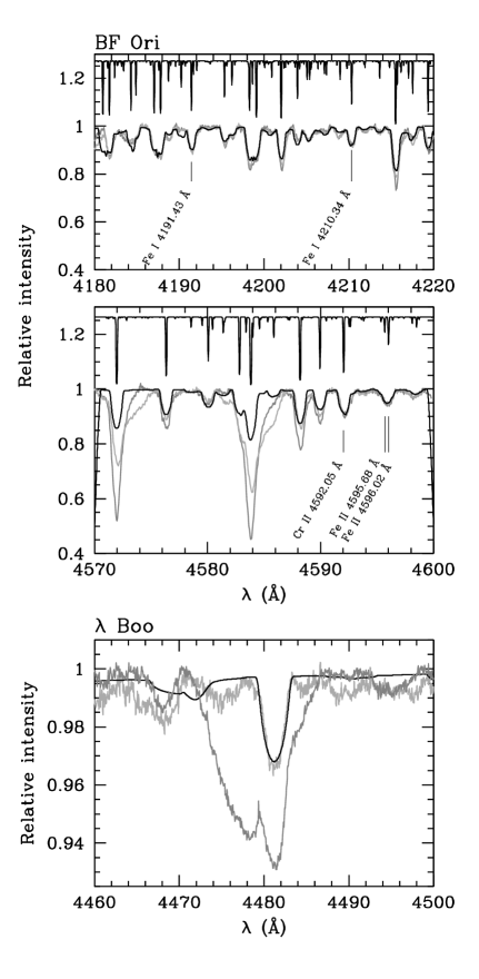
Figure 3: Top: Two sections of the UES/WHT spectra of BF Ori along with the synthetic spectrum. The spectra plotted in dark-grey and light-grey solid lines –both of them with their continuum normalized to an intensity of 1.0– were obtained on 25 October 1998 and 30 January 1999, respectively. The synthetic spectrum, computed for $T_{\rm eff}=8970$ K, $\log g_{*}=3.83$ and [M/H]=+0.20 and broadened with a rotation profile $v\sin i=38$ km/s has been plotted as a black solid line overimposed to the observed spectra. In the upper part of each panel we show the synthetic unbroadened spectrum –not to scale– for comparison. Bottom: Two spectra of $\lambda$ Boo around the Mg ii doublet obtained on 16 May 1998 (light grey) and 29 July 1998 (dark grey). The first one is best fitted with [Mg/H]=$-2.0$, whereas the latter shows traces of high circumstellar activity. See text for further details.

Metal abundances are determined by comparing the profiles of lines (or blends) extracted from the high-resolution spectra, with synthetic spectra computed using the ATLAS9 and SYNTHE codes by Kurucz (1993). In this work we have used the GNU Linux version of the codes prepared by Luca Sbordone, Piercarlo Bonifacio and Fiorella Castelli, available online (Sbordone et al. 2004).

Model atmospheres provided by Castelli & Kurucz (2003) are used as one of the inputs for the synthesis. These models have more accurate solar abundances, were computed with new opacity distribution functions (ODFs) and contain further improvements upon previous ODFs Kurucz’s models (see the paper by Castelli & Kurucz (2003) for details). The ATLAS9 code allows to compute, for a given metallicity, a model atmosphere for any value of the effective temperature and gravity from a ‘close’ model already present in the Castelli & Kurucz’s grids. In fact, this step had to be done for all the stars in our sample because the corresponding model atmospheres did not exist for their values of $T_{\rm eff}$ and $\log g_{*}$.

The spectral synthesis was carried out using SYNTHE, which is actually not a single code, but a suite of programmes. Apart from the model atmosphere –which contains, among other things, the atomic fractions of the different elements– the list of the atomic and molecular transitions and the spectral range to be synthetized are also read. SYNTHE computes the excitation and ionization populations of neutrals and ions and then produces the final spectrum. A special module of SYNTHE computes intensities at several inclinations in the atmosphere and uses these, along with the value of $v\sin i$ (see Table 1), to simulate the spectrum of a rotating star.

Spectra corresponding to the same $T_{\rm eff}$ and $\log g_{*}$ are computed for different metallicities and a comparison is done with the observed spectrum. Most of the stars in the sample have large values of the projected rotational velocity, therefore it is impossible to analyse individual lines and only an average value of the metallicity can be extracted. Two regions have been explored to estimate metallicities, namely, that between 4150 and 4280 Å and the one between 4450 and 4520 Å. In a few stars, those with low or moderate values of $v\sin i$, individual abundances for each chemical element could be derived from the spectra, this is the case for HR 5422 A and BF Ori, and to a less extent, that of stars with $v\sin i$ less than around 150 km/s. In this work only average abundances, even for the low-$v\sin i$ objects, were computed.

Some stars in the sample show various and complex degrees of variability; therefore it is important, whenever it is possible, to compare all the spectra available for a given object and select those spectral features that present little or no variation from one epoch to another. In Figure 3 we show two examples of how important this can be. The top part of the plot shows two regions of high-resolution spectra of BF Ori. The spectra taken on 25 October 1998 (dark-grey line) and 30 January 1999 (light-grey line) are shown together with the synthetic spectrum, which has been overplotted as a black solid line. In the upper part of each panel, the unbroadened spectrum shows how many transitions contribute to each blend. It is apparent in both sections plotted, especially in the second panel, covering the interval 4570–4600 Å, how some lines change dramatically from one epoch to another. Other features, which have been labelled with the identification of the most intense line in the blend, remain almost unchanged. The panel at the bottom shows two spectra of $\lambda$ Boo around the Mg ii doublet at 4481.13–4481.33 Å obtained on 16 May 1998 (light grey) and 29 July 1998 (dark grey). The first one is best fitted with [Mg/H]=$-2.0$, whereas the latter shows traces of high circumstellar activity. No attempt was made to obtain any value of the abundance from this spectrum.

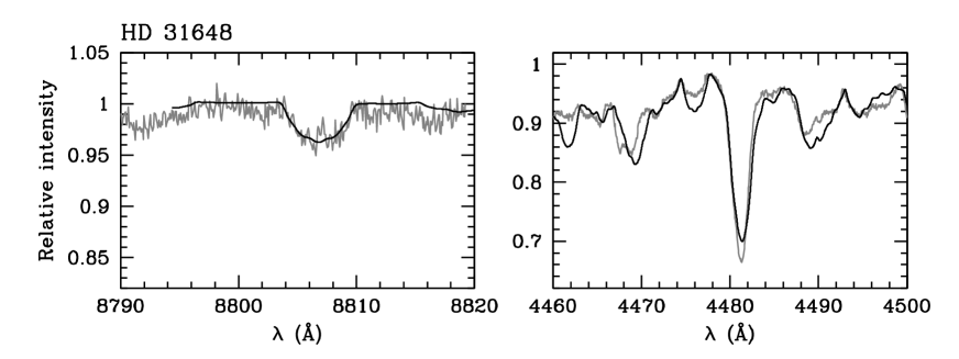
Figure 4: Two regions of the spectrum of HD 31648 around the Mg i line at 8806.76 Å, and the Mg ii doublet at 4481.2 Å, respectively (grey lines). The Mg i profile is best fitted by a model with [Mg/H]=$-0.10$, whereas the Mg ii doublet is best reproduced with a synthetic model with [Mg/H]=$+0.50$ (black lines).

Figure 4 is also very illustrative of another difficulty to estimate the metal abundances for these stars: in some cases, for a given object, lines of the same element in different ionization states, are fitted by synthetic spectra with very different metal abundances. The plot shows two regions of the spectrum of HD 31648, namely around the Mg i line at 8806.76 Å, and around the Mg ii doublet at 4481.2 Å, respectively. The observations are not simultaneous, the Mg i profile is best fitted by a model with [Mg/H]=$-0.10$, whereas the Mg ii doublet is best reproduced with a synthetic model with [Mg/H]=$+0.50$. Such a discrepancy could be attributed to circumstellar contamination of the line in the latter case.

4.4 Iterations

As we mentioned at the beginning of this Section, the determination of the effective temperature was done by comparing the SED of each star with synthetic models with [M/H]=0.0. The first determination of the stellar gravity, following the flow chart shown in Fig. 1, also assumed solar metallicity. The pair ($T_{\rm eff}$, $\log g_{*}$) was used to extract the metallicity. When the value of the metal abundance obtained was different by more than 0.30 dex from the solar one, we iterated the whole process, i.e. a new effective temperature was estimated and a new gravity was found, using in both cases models and synthetic profiles computed with the new metallicity. It turned out that for metallicity differences as large as 0.80, the new effective temperature did not differ from the original determination, therefore only the gravity was recomputed for those stars. A full iteration, i.e. the estimation of new values of $T_{\rm eff}$ and $\log g_{*}$, was done for $\lambda$ Boo. One iteration cycle was sufficient to reach the final results.

4.5 Masses, luminosities, ages and distances

As it can be seen at the bottom of Fig. 1, the knowledge of the effective temperature, gravity and metal abundance allows us to place the star in an HR diagram $\log g_{*}-\log T_{\rm eff}$ and superimpose the appropriate set of evolutionary tracks and isochrones for that specific metallicity. This gives directly –or after a simple interpolation between the tracks and isochrones enclosing the position of the star– the stellar mass and the age. In addition, since there is a one-to-one correspondence between a pair $(T_{\rm eff},\,g_{*})$ on a given track and a pair $(T_{\rm eff},\,L_{*}/L_{\odot})$, one can also estimate the stellar luminosity in solar units, and if the observed –dereddened– stellar flux, $F_{*}$, is known through the SED, then, an estimation of the distance can also be done. The values of $F_{*}$ are taken from Merín (2004) or determinations carried out in this work. $F_{*}$ is computed by fully integrating the flux of the dereddened synthetic Kurucz model that is considered to best fit the photospheric part of the SED.

The evolutionary tracks for a scaled solar mixture from the Yonsei-Yale group (Yi et al. 2001) – Y² in their notation – have been used in this work. The Y² set contains tracks up to $M$=5.2 M_⊙, therefore, the tracks from Siess et al. (2000) for masses above that value were used in a few cases (see subsection 5.2 for details).

Table 2: Effective temperatures, gravities and metallicities.

Star	$T_{\rm eff}$ (K)	$\log g_{*}$
HD 58647	105001	$3.33\pm 0.05$
HD 150193	89701	$3.99\pm 0.12$
HD 179218	95001	$3.91\pm 0.07$
HD 190073	95001	$3.37\pm 0.08$
HR 26 A	114002	$4.08\pm 0.05$
AS 442	110007	$3.79\pm 0.10$
BD+31 643	154001	$3.75\pm 0.05$
V346 Ori	97507	$3.96\pm 0.11$
V350 Ori	89707	$4.07\pm 0.12$

Star	$T_{\rm eff}$ (K)	$\log g_{*}$	[M/H]
HD 31648	82507	$4.00\pm 0.20$	$0.00\pm 0.05$
HD 163296	92507	$4.07\pm 0.09$	$+0.20\pm 0.10$
HR 10	97507	$3.72\pm 0.10$	$+0.20$:
HR 2174	89701	$3.08\pm 0.12$	$0.00\pm 0.10$
HR 4757 A	104002,7	$4.06\pm 0.05$	$+0.10\pm 0.10$
HR 5422 A	102507	$4.08\pm 0.06$	$+0.20\pm 0.10$
HR 9043	75703	$3.85\pm 0.10$	$0.00\pm 0.10$
$\lambda$ Boo	87504	$4.10\pm 0.12$	$-1.50\pm 0.20$
VX Cas	100007	$4.27\pm 0.05$	$0.00\pm 0.10$
SV Cep	102505,7	$4.25\pm 0.10$	$+0.10\pm 0.10$
49 Cet	95007	$4.30\pm 0.11$	$+0.10\pm 0.10$
24 CVn	90007	$3.81\pm 0.13$	$+0.80\pm 0.10$
51 Oph	102507	$3.57\pm 0.06$	$+0.10\pm 0.10$
T Ori	97507	$4.03\pm 0.10$	$+0.10\pm 0.10$
BF Ori	89701	$3.83\pm 0.12$	$+0.20\pm 0.05$
UX Ori	84601	$3.89\pm 0.15$	$0.00\pm 0.10$
XY Per	97507	$3.86\pm 0.16$	$+0.80$:
VV Ser	138006,7	$4.02\pm 0.15$	$0.00$:
17 Sex	95201	$3.19\pm 0.10$	$+0.10\pm 0.10$
RR Tau	100007	$3.31\pm 0.13$	$+0.10\pm 0.05$
WW Vul	89701	$3.90\pm 0.20$	$+0.50\pm 0.10$

Notes to Table 2: The effective temperatures are from ¹Merín (2004), ²Gerbaldi et al. (2001), ³Paunzen et al. (2006), ⁴adopted as a mean of the values proposed by Venn & Lambert (1990) and Adelman et al. (2002), ⁵Mora et al. (2004), ⁶Hernández et al. (2004), ⁷this work.

5 Results

5.1 Gravities and metallicities

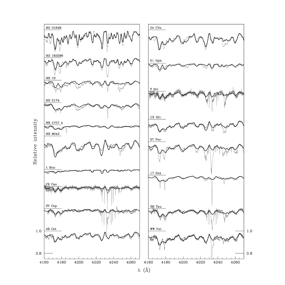
Figure 5: Selected observed spectra of the stars studied in this paper (grey lines) and synthetic spectra (black lines overplotted on each spectrum) computed with the metallicities [M/H] given in Table 2. The spectral range is 4160-4270 Å. All the spectra have been normalized and plotted on the same scale, and have been shifted upwards with respect to the lowest ones. The small horizontal bars below the identification of the stars mark the intensity level unity for each pair of spectra. To have an idea of the range of intensities each spectrum covers, we have indicated the levels $I\!=\!0.8$ and $I\!=\!1.0$ corresponding to 49 Cet and WW Vul in both panels. The spectra of HR 5422 A, BF Ori and VV Ser are not shown; the first two stars have low values of $v\sin i$, therefore the lines are extremely narrow and the plots would look clumsy, the latter has a rather noisy spectrum and the resuls are uncertain. Two sections of the spectrum of BF Ori and the corresponding synthetic spectrum are shown in Fig. 3.

Table 2 shows the values of the effective temperature, gravity and metallicity (the latter when high-resolution observations were available) for the stars in the sample. In three cases, namely HR 26 A, HR 9043 and $\lambda$ Boo, specified in the table, values of $T_{\rm eff}$ obtained by other authors with a methodology different from that of Merín (2004) or this work have been taken; for the first two stars the calibrations used in those papers gave more accurate results than ours, whereas for $\lambda$ Boo the value adopted is a mean of the effective temperatures from two works where detailed studies of this star are done. The fourth column of the lower part of the table gives a generic value of [M/H], estimated by comparing the observed spectra with the synthetic ones and trying to mach the shape and depth of the non-variable blends composed of many broadened individual lines. The determinations of [M/H] for HR 10, XY Per and VV Ser are marked with a colon, indicating that they are very uncertain given the large amount of circumstellar lines contaminating the photospheric spectra, or the low signal-to-noise ratio in the spectra of the latter object; therefore these values should be taken with caution.

In Fig. 5 we show selected spectra (grey lines) of all the stars in the sample, apart from a few exceptions, for which an estimation of the metal abundance has been possible and the synthetic spectra (black lines) computed using the values of $T_{\rm eff}$, $\log g_{*}$ and [M/H] given in Table 2. All the spectra are plotted on the same scale. To show all together in the same graph we have shifted them upwards by different amounts with respect to the lowest one in each panel. The short horizontal bars mark where the intensity unity is placed. Each observed spectrum has been normalized to its corresponding synthetic spectrum. The fits to HR 10 and XY Per are just tentative, showing how difficult is to find a region in the spectra not contaminated by circumstellar lines.

5.2 Masses, luminosities, ages and distances

In Table 3 we give the results of the determination of masses, luminosities, ages and distances, following the procedure illustrated in Fig. 1 and outlined in subsection 4.5. The uncertainties for each value correspond to the propagation of the errors $\pm\sigma(\log g_{*})$. Note that in some special cases, e.g. the masses of VV Ser or T Ori, these uncertainties can have the same sign, if the position in the HR diagram is such that the points $(\log T_{\rm eff},\log g_{*}+\sigma(\log g_{*}))$ and $(\log T_{\rm eff},\log g_{*}-\sigma(\log g_{*}))$ fall on tracks with masses both larger (or smaller) than those corresponding to the point $(\log T_{\rm eff},\log g_{*})$ itself (see Fig. 6). For the nine stars at the upper part of Table 2, for which the computation of metal abundances was not feasible, tracks with solar metallicity have been used. The second column of the table lists the values of $F_{*}$ used to estimate the distance from the stellar luminosity. The last two columns show the distances derived from Hipparcos parallaxes (van Leeuwen, 2007) (col. 7) and taken from other sources (col. 8). For the former ones, only parallaxes whose uncertainty $\sigma(\pi)$ is such that $\sigma(\pi)/\pi\leq 0.15$ have been considered. In subsection 6.3 we discuss in detail the values of our estimation of distances –actually, as we will see, upper limits in some cases– compared with other determinations.

From the Y² set, the tracks with $Z\!=\!0.02$ (solar) have been used for those stars with metallicities [M/H] between $-0.10$ and $+0.10$. Assuming that the relationship Fe/Fe_⊙=X/X_⊙ holds (in number of particles), where X means any element with atomic number larger than 3, the tracks corresponding to [M/H]=$+0.20$ would be those with $Z\!=\!0.03$. Since these tracks are not computed in the original set, the results shown in Table 3 are the average of the values extracted using the tracks with $Z\!=\!0.02$ and $Z\!=\!0.04$. For those stars with [M/H]=$+0.50$ the set $Z\!=\!0.06$ was used. Finally for $\lambda$ Boo, we used the tracks with $Z\!=\!0.0004$, which would correspond to [M/H]=$-1.7$. For HD 58647 and BD+31 643 there are no high-resolution observations available to estimate metallicities, therefore we assumed solar abundances to estimate their stellar parameters; on the other hand, for HR 2174, 17 Sex and RR Tau the metallicities found are solar or very close to it. The five objects have in common that their locations in the HR diagram give masses above 5.2 $M_{\odot}$, which is the maximum in the Y² set, therefore, only for these stars we used the Siess et al. tracks with solar metallicity.

Table 3: Stellar fluxes, masses, luminosities, ages and distances.

Star	$F_{*}$ (W m-2)	$M_{*}/M_{\odot}$	$L_{*}/L_{\odot}$	Age (Myr)	$d$ (pc)	$d_{\rm Hip}$ (pc)	$d_{\rm other}$ (pc)
HD 31648	3.308$\times 10^{-11}$	1.97${}^{+0.04}_{+0.45}$	21.9${}^{-7.8}_{+20.7}$	6.7${}^{+1.0}_{-3.3}$	146${}^{-29}_{+57}$	137${}^{+31}_{-21}$
HD 58647	9.940$\times 10^{-11}$	5.99${}^{-0.36}_{+0.38}$	911.2${}^{-113.4}_{+221.2}$	0.4${}^{+0.1}_{-0.1}$	543${}^{-35}_{+62}$
HD 150193	2.825$\times 10^{-11}$	2.22${}^{-0.04}_{+0.27}$	36.1${}^{-9.2}_{+17.5}$	5.0${}^{+0.5}_{-1.5}$	203${}^{-28}_{+44}$
HD 163296	6.583$\times 10^{-11}$	2.25${}^{+0.11}_{+0.07}$	34.5${}^{-5.1}_{+9.3}$	5.0${}^{-0.3}_{-0.6}$	130${}^{-10}_{+16}$	119${}^{+12}_{-10}$
HD 179218	4.996$\times 10^{-11}$	2.56${}^{-0.16}_{+0.21}$	63.1${}^{-12.8}_{+17.0}$	3.3${}^{+0.7}_{-0.7}$	201${}^{-22}_{+25}$
HD 190073	2.575$\times 10^{-11}$	5.05${}^{-0.47}_{+0.54}$	470.8${}^{-88.2}_{-189.2}$	0.6${}^{+0.2}_{-0.2}$	767${}^{-76}_{+139}$
HR 10	1.737$\times 10^{-10}$	3.30${}^{-0.37}_{+0.43}$	140.3${}^{-41.9}_{+59.2}$	1.8${}^{+0.5}_{-0.5}$	161${}^{-26}_{+31}$	176${}^{+24}_{-19}$
HR 2174	1.515$\times 10^{-10}$	6.82${}^{-0.93}_{+1.02}$	1012.7${}^{-351.4}_{+217.2}$	0.2${}^{+0.1}_{-0.1}$	463${}^{-89}_{+47}$
HR 9043	8.784$\times 10^{-11}$	2.07${}^{-0.21}_{+0.27}$	23.7${}^{-6.7}_{+10.0}$	5.5${}^{+2.0}_{-1.7}$	93${}^{-14}_{+18}$	88${}^{+4}_{-3}$
AS 442	9.753$\times 10^{-12}$	3.54${}^{-0.37}_{+0.44}$	207.2${}^{-60.1}_{+85.2}$	1.5${}^{+0.5}_{-0.5}$	826${}^{-130}_{+155}$
BD+31 643	2.483$\times 10^{-10}$	6.15${}^{-0.29}_{+0.29}$	1663.5${}^{-234.9}_{+329.8}$	0.4${}^{+0.1}_{-0.1}$	464${}^{-34}_{+36}$
$\lambda$ Boo	6.240$\times 10^{-10}$	1.66${}^{-0.16}_{+0.19}$	19.1${}^{-6.1}_{+9.0}$	2.8${}^{+1.1}_{-0.8}$	31${}^{-5}_{+7}$	30$\pm 1$
VX Cas	2.589$\times 10^{-12}$	2.33${}^{-0.03}_{+0.14}$	30.8${}^{-5.7}_{+5.8}$	6.4${}^{+4.0}_{-1.5}$	619${}^{-60}_{+58}$		7601,3
SV Cep	3.390$\times 10^{-12}$	2.45${}^{-0.08}_{+0.26}$	37.5${}^{-5.1}_{+14.5}$	5.2${}^{+1.4}_{-2.1}$	596${}^{-43}_{+106}$		4403
24 CVn	4.686$\times 10^{-10}$	2.64${}^{-0.11}_{+0.42}$	65.9${}^{-19.1}_{+38.0}$	3.1${}^{+0.6}_{-1.1}$	67${}^{-11}_{+17}$	55$\pm 1$
51 Oph	4.991$\times 10^{-10}$	4.22${}^{-0.30}_{+0.33}$	312.3${}^{-62.3}_{+72.0}$	0.7${}^{+0.4}_{-0.5}$	142${}^{-15}_{+15}$	124$\pm 4$
T Ori	7.242$\times 10^{-12}$	2.42${}^{+0.06}_{+0.17}$	50.2${}^{-9.4}_{+17.4}$	4.0${}^{-0.1}_{-0.8}$	472${}^{-46}_{+76}$		4601
BF Ori	5.445$\times 10^{-12}$	2.61${}^{-0.25}_{+0.41}$	61.6${}^{-20.2}_{+32.4}$	3.2${}^{+1.3}_{-0.9}$	603${}^{-109}_{+142}$		4502, 4303
UX Ori	4.414$\times 10^{-12}$	2.26${}^{-0.25}_{+0.52}$	36.8${}^{-13.7}_{+30.5}$	4.5${}^{+2.0}_{-2.3}$	517${}^{-108}_{+182}$		4601, 4002, 3403
V346 Ori	5.752$\times 10^{-12}$	2.52${}^{-0.11}_{+0.31}$	61.4${}^{-15.8}_{+27.3}$	3.5${}^{+0.6}_{-1.1}$	586${}^{-81}_{+118}$		4502
V350 Ori	1.741$\times 10^{-12}$	2.16${}^{+0.13}_{+0.13}$	29.29${}^{-5.8}_{+11.6}$	5.5${}^{-0.1}_{-1.0}$	735${}^{-77}_{+133}$		4601, 4502
XY Per	2.290$\times 10^{-11}$	2.79${}^{-0.36}_{+0.59}$	85.6${}^{-34.0}_{+64.3}$	2.5${}^{+1.5}_{-0.8}$	347${}^{-78}_{+190}$		1201, 3502, 1603
VV Ser	2.869$\times 10^{-11}$	3.95${}^{+0.15}_{+0.41}$	336.2${}^{-89.4}_{+117.2}$	1.2${}^{+0.1}_{-0.5}$	614${}^{-88}_{+99}$		4401, 3303, 2304
17 Sex	1.757$\times 10^{-10}$	6.35${}^{-0.74}_{+0.80}$	940.5${}^{-277.2}_{+295.8}$	0.3${}^{+0.1}_{-0.1}$	415${}^{-30}_{+61}$
RR Tau	5.673$\times 10^{-12}$	5.79${}^{-0.94}_{+0.99}$	780.5${}^{-351.9}_{+446.7}$	0.4${}^{+0.3}_{-0.2}$	2103${}^{-544}_{+535}$		8001, 6002
WW Vul	3.315$\times 10^{-12}$	2.50${}^{-0.06}_{+0.48}$	50.0${}^{-19.11}_{+44.5}$	3.7${}^{+3.7}_{-1.7}$	696${}^{-149}_{+261}$		5501, 5342
HR 26 A	2.582$\times 10^{-10}$	3.08${}^{-0.07}_{+0.07}$	106.9${}^{-14.2}_{+15.7}$	175${}^{-23}_{+14}$	115${}^{-8}_{+8}$	94$\pm 3$
		3.01${}^{+0.10}_{-0.01}$	104.0${}^{-7.8}_{+11.9}$	2.6${}^{-0.2}_{-0.1}$	114${}^{-4}_{+6}$
HR 4757 A	2.647$\times 10^{-9}$	2.74${}^{-0.06}_{+0.07}$	69.0${}^{-8.9}_{+9.7}$	260${}^{-24}_{+14}$	29${}^{-2}_{+2}$	27$\pm 1$
		2.64${}^{+0.04}_{+0.02}$	64.0${}^{-4.2}_{+10.7}$	3.2${}^{-0.1}_{-0.1}$	28${}^{-1}_{+2}$
HR 5422 A	1.439$\times 10^{-10}$	2.66${}^{-0.07}_{+0.08}$	60.4${}^{-9.8}_{+11.0}$	267${}^{-39}_{+23}$	116${}^{-10}_{+10}$	110$\pm 5$
		2.59${}^{+0.09}_{+0.01}$	58.5${}^{-5.7}_{+8.7}$	3.4${}^{-0.2}_{-0.1}$	114${}^{-6}_{+8}$
49 Cet	2.064$\times 10^{-10}$	2.17${}^{-0.03}_{+0.06}$	21.8${}^{-1.0}_{+3.9}$	61${}^{-46}_{+119}$	58${}^{-1}_{+5}$	59$\pm 1$
		2.15${}^{-0.01}_{+0.11}$	21.6${}^{-0.8}_{+4.4}$	8.9${}^{+6.1}_{-2.4}$	58${}^{-1}_{+6}$

Notes to Table 3: A discussion on the derivation of the distances given in col. 6 is done in subsection 6.3. The distances given in col. 8 are taken from the works by ¹Hernández at al. (2004), ²Blondel & Tjin A Djie (2006), ³Manoj et al. (2006) and ⁴Eiroa et al. (2008); see those works for the original references. For HR 26 A, HR 4757 A, HR 5422 A and 49 Cet we give the solutions derived using both Post-MS and PMS tracks, respectively (see subsection 6.4).

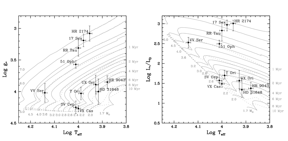
Figure 6: Left: $\log g_{*}-\log T_{\rm eff}$ HR diagram showing the position of the stars with metallicity [M/H]= 0.00 and $+0.10$. Right: The corresponding $\log L_{*}/L_{\odot}-\log T_{\rm eff}$ HR diagram for the same stars. There is a one-to-one correspondence between a point $(\log T_{\rm eff},\log g_{*})$ and a point $(\log T_{\rm eff},\log L_{*}/L_{\odot})$. This allows the estimation of masses, ages and luminosities provided the effective temperature and gravity are known. The sets of PMS tracks (solid lines) and isochrones (dashed lines) for solar metallicity from Yi et al. (2001; masses up to 4.5 $M_{\odot}$) and Siess et al. (2000; 5.0, 6.0 and 7.0 $M_{\odot}$) have been used in both plots. The stars HR 4757 A and 49 Cet are not included in this plot. Their position in the HR diagram is discussed in subsection 6.4. See text for details.

In Fig. 6 we show, at the left, the $\log g_{*}$ – $\log T_{\rm eff}$ HR diagram for the stars with metallicities between [M/H]=$-0.10$ and $+0.10$, where tracks and isochrones for solar metallicity have been superimposed, and at the right, the corresponding $\log L_{*}/L_{\odot}$ – $\log T_{\rm eff}$ HR diagram. The vertical error bars in the points $(\log T_{\rm eff},\log g_{*})$ correspond to those listed in Table 2 whereas those in the points $(\log T_{\rm eff},\log L_{*})$ are the propagation of the former from the first HR diagram to the second, hence their different size up and down for a given object. A common horizontal error bar of $\pm 0.01$ dex has been assigned to the logarithm of effective temperatures, which corresponds to $\pm 200$ K at $T_{\rm eff}$=10000 K.

6 Discussion

One important fact to bear in mind before starting the discussion is that the results concerning the stellar mass, luminosity and age given in Table 3 are distance-independent determinations. Let us remember that taking advantage of the knowledge of the stellar gravity we are able to extract the mass and the age from a $\log g_{*}$ – $\log T_{\rm eff}$ HR diagram, and then the luminosity from the corresponding point in the $\log L_{*}/L_{\odot}$ – $\log T_{\rm eff}$ HR diagram.

In other works, e.g. those from Gerbaldi et al. (2001), Hernández et al. (2004) and Manoj et al. (2006), the authors extract these parameters from a $\log L_{*}/L_{\odot}$ – $\log T_{\rm eff}$ HR diagram, which implies a knowlegde of the distance to the star, this being quite an uncertain parameter in many occasions. Also, in the three works mentioned above, solar metallicity is assumed for all the stars, whereas in our case, specific tracks for each metallicity are used according to the abundance estimated for each object. The different approaches of both formalisms makes it difficult a comparison among the values of $M_{*}/M_{\odot}$, $L_{*}/L_{\odot}$ and age from our work and those from other authors. That is the reason why in Table 3 we only provide for comparison values of distances from other works, which are discussed later (see subsection 6.3), whereas we do not include any value of masses, luminosities and ages other than those found in this paper. A detailed comparison of results for these parameters would be lengthy and cumbersome.

6.1 General considerations on the effective temperatures

The whole exercise carried out in this paper can be considered as a work of basic astrophysics, in the sense that it concerns the determination of fundamental parameters of a particular class of stars. The process has been far from simple, due to the very nature of the objects studied, i.e. most of them are not ‘normal’ stars in the sense that their environment has a clear influence on the photometric and spectroscopic properties.

As we mentioned, the correct determination of the effective temperature, the only initial parameter required to start the whole process, is a key problem of this study. The calculation of $T_{\rm eff}$ hinges on the fit of the SED, using synthetic models, from short wavelengths (optical or UV) to a wavelength in the infrared, $\lambda_{0}$, where a change in the slope indicates that the contribution from the disk starts to be noticeable. The photospheric part of the SED can be affected by circumstellar (and interstellar) extinction, disk occultation and, in addition, there can be non-photospheric contributions in the UV (e.g. emission from accretion shocks or hot winds). In the determination of the effective temperatures carried out both by Merín (2004) and in this work, done by fitting Kurucz models to the observed SEDs and given in Table 2, it was assumed that the spectral energy distribution from the UV to $\lambda_{0}$, originates entirely in the stellar photosphere. This hypothesis underlies the whole procedure and should be critically assessed in each case. In subsection 6.4 we analyse in detail –among other stars– VV Ser and RR Tau, for which the determination of the effective temperature is especially problematic.

6.2 Comparison with other abundance determinations

Apart from the values of [M/H] around +0.80, for 24 CVn and XY Per, +0.50 for WW Vul, and the already well-known low metallicity of $\lambda$ Boo, the remaining values of the abundances found in this work are solar or fairly close to it. In addition to the stars analysed in this paper, the two HAeBe stars studied by our group (Merín et al. 2004), namely HD 34282 and HD 141569, show metallicities lower than solar, $-0.80$ and $-0.50$ respectively. No trend in the behaviour of the metallicities is observed in the results for our sample.

As we mentioned in the Introduction, Acke & Waelkens (2004) carried out an abundance study of 24 Herbig Ae/Be and Vega-type stars searching for the $\lambda$ Bootis phenomenon. For 20 of these stars the projected rotational velocities, $v\sin i$, are less than 100 km/s, therefore the authors were able to determine elemental abundances, instead of average values as in our case. Stellar gravities were not estimated in that paper. In order to compare their results with ours we have computed a ‘mean’ metal abundance from those individual values. Details on how this was done are given in Appendix A.

Guimarães et al. (2006), as a result of a study of the accretion in Herbig Ae/Be stars, also determined stellar gravities and metal abundances for 12 stars. The methodology of their work is almost identical to the one we have used in this paper and also in the analysis of HD 34282 and HD 141569 (Merín et al. 2004). They provide results for [Fe/H]. Apart from the extreme Fe abundance of HD 100546 (not studied in this work), namely $-1.4$, in agreement with the value $-1.30$ given by Acke & Waelkens (2004), the abundances for their sample vary from $-1.0$ to $+0.5$.

The three samples are not large enough to draw any definitive statistical conclusion, although it is apparent that both in our work and in Acke & Waelkens’ (2004) the majority of the stars tend to lie around metallicities close to the solar one. The highest metallicities found in any of the three works are around +0.80 whereas the lowest ones are below $-1.0$.

There is only one star in our sample in common with Acke and Waelkens’, namely HD 31648 (they found [M/H]=$+0.33\pm 0.08$ and [Fe/H]=$+0.07\pm 0.10$), and another one with Guimarães et al., namely HD 163296 (their result is [Fe/H]=$+0.50\pm 0.10$). Our results are [M/H]=$0.00\pm 0.05$ for HD 31648 and [M/H]=$+0.20\pm 0.10$ for HD 163296, in both cases somewhat lower than the determinations of those two works.

6.3 The estimation of the distances

Since the estimation of the distances hinges first on the determination of the point ($\log T_{\rm eff}$, $\log g_{*}$) and then in the ‘translation’ of this point to a value of ($\log T_{\rm eff}$, $\log L_{*}/L_{\odot}$), any error in the derivation of the effective temperature or the gravity would propagate to the final value of the distance.

Figure 7: Plot showing the Hipparcos distances (x-axis) for the 11 stars in the sample with reliable parallaxes (see text for details), plotted against the corresponding distances estimated in this work (y-axis).

As it can be seen in Table 3 there are 11 stars for which Hipparcos parallaxes such that $\sigma(\pi)/\pi\leq 0.15$ –i.e. implying reliable distances– are available. The comparison between our estimations and the Hipparcos-derived distances, illustrated in Fig. 7, shows that in all those cases both determinations agree to within the uncertainties. This is an additional indication of the internal coherence of the overall results.

The remaining stars in Table 3 either do not have Hipparcos measurements or if they do, the large uncertainties make them unusable. Instead, their distances have been estimated using a variety of methods; in most cases the numbers found in the literature are just the distances to the clouds where they could be embedded, which are, obviously, rough approximations. In col. 8 of the Table we give results from the compilations made by Hernández et al. (2004), Blondel & Tjin A Djie (2006) and Manoj et al. (2006). It can be seen that in some cases those distances are comparable to our results (e.g. T Ori, UX Ori, XY Per, WW Vul) but for other stars the discrepancies are large. We can see a systematic trend between our results (col. 6) and those from other authors (col. 8): out of 11 cases, in nine of them the distances derived in this work are larger than the distance to the parent cloud; the case of RR Tau is especially noticeable.

After exploring what might be the origin of this, we think that there is an important fact that should be taken into account in interpreting these discordant results. Note that to derive the distance $d$, we have used the well-known expression $L_{*}\!=\!4\pi d^{2}F_{*}$, where $L_{*}$ is the stellar luminosity and $F_{*}$ is the observed photospheric flux, corrected for reddening. To provide the correct distance, that simple expression must contain the total flux, i.e. it is implicitly assumed that the whole stellar photosphere is visible to the observer. If this does not occur, $F_{*}$ would be underestimated and, since the stellar luminosity has been fixed, the implied distance would be larger than the real one. It could happen that, if the inclination of the circumstellar disk is high or the opacity of part of its material is very large (or both), the disk would block a fraction $\alpha$ of the stellar light, allowing only a fraction $F_{*}=(1-\alpha)F_{*}({\rm total})$ to reach the observer. Since the material of the disk can be very inhomogeneous, $\alpha$ would parameterize a sort of mean ‘filling factor’ for the occultation and obscuration of the stellar light caused by extremely high values of the extinction (note that the observed flux $F_{*}$ can still be affected by circumstellar and interestellar extinction). In addition, as we pointed out in 4.1, the SED is built taking the brightest photometry among the available observations, which could not necessarily correspond to the true maximum brightness of the star: if that is the case, the photospheric flux would be also less than the real one.

These arguments would put in agreement the discrepancies we mentioned above. In subsection 6.4 we discuss in detail the cases of VV Ser and RR Tau, and we see how this effect could have some impact in our calculations.

The bottom line of this discussion is that the distances derived in this work and given in col. 6 of Table 3 should be used with caution. In particular, for those objects with high values of the extinction or high inclination angles of their disks (e.g. almost edge-on disks, as it happens in the UXORs), they must be taken as upper limits of the actual distances.

6.4 Notes on individual stars

6.4.1 VV Ser

This star is an intriguing HAeBe object. The determinations of its parameters found in the literature are discrepant, showing large differences in many occasions. A summary of the results on the spectral type, luminosity class and rotational velocities can be found in Table 1 of the paper by Ripepi et al. (2007). Assignations such us A0 V, A3 II, A2 III or B6 to the spectral type and values of $v\sin i$ from 85 to 229 km/s can be found (see references in the paper by Ripepi et al.). Concerning the effective temperature, a wide range from $9000\pm 1000$ K (Ripepi et al. 2007) to 13800 K (Hernández et al. 2004) is found.

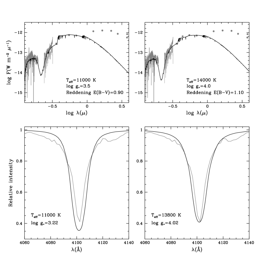
Figure 8: Top: The observed spectral energy distribution of VV Ser (grey lines and dots) and two fits to the photospheric contribution (black lines). The UV spectra were obtained with the International Ultraviolet Explorer (IUE); the leftmost –and more noisy– spectrum is SWP 48866 (dark grey, obtained on 7/10/1993)) and the two spectra to its right are LWP 26520 (dark grey, 7/10/1993), and a merge of LWP 28921 and LWP 28931 (light grey, 18–19/10/1994); these are the only spectra obtained by IUE of this object. The optical $UBVRI$ photometry was obtained on 24/10/1998. Top left: The SED has been fitted by a Kurucz model with $T_{\rm eff}\!=\!11000$ K, $\log g_{*}\!=\!3.5$, reddened with $E(\!B-\!V)\!=\!0.90$. Top right: The SED has been fitted by a Kurucz model with $T_{\rm eff}\!=\!14000$ K, $\log g_{*}\!=\!4.0$, reddened with $E(\!B-\!V)\!=\!1.10$. Bottom: The observed H$\delta$ line of VV Ser (grey line) and two fits with synthetic models (black lines). Bottom left: the best fit achieved using $T_{\rm eff}\!=\!11000$ K and $\log g_{*}\!=\!3.22$. Bottom right: the best fit for $T_{\rm eff}\!=\!13800$ K and $\log g_{*}\!=\!4.02$.

The estimates of the distance to the Serpens molecular cloud, where there would be a possibility that the star is embedded into, have also many uncertainties. The most recent studies converge to a somewhat shorter distance: $225\pm 55$ pc for the front edge of the particular region of the cloud studied (south of the cloud core) and a depth of 80 pc for the cloud complex (Straižys et al. 2003). Eiroa et al. (2008) assign a distance of $\sim\!230\pm 20$ to the Serpens cloud (see that reference for a complete review on the properties of this region). There are no direct determinations of the distance to VV Ser itself, and the values found in the literature are linked to the distance to the cloud.

The initial value of $T_{\rm eff}$ for VV Ser we took to compute the stellar parameters, according to the scheme presented in Section 4, was 11000 K, obtained by Merín (2004), which is in between the available determinations. The comparison of the synthetic Balmer profiles with the observed ones led to a value of $\log g_{*}=3.22\pm 0.12$, which implied the following set of parameters: $M_{*}\!=\!7.22^{-0.95}_{+1.00}$ $M_{\odot}$, $L_{*}\!=\!1638^{-467}_{+261}$ $L_{\odot}$, Age=0.2${}^{+0.1}_{-0.1}$ Myr and, after combining the luminosity and the observed flux, an upper limit to the distance $d=2224^{-344}_{+170}$ pc.

In Fig. 8 (top) we show the observed SED of VV Ser from the ultraviolet to the infrared, along with two fits to the photospheric part, which covers the interval between 1200 Å and 9000 Å ($I$ band); from this wavelength onwards, the contribution from the disk dominates. Note that the ultraviolet spectra, obtained with the IUE observatory, are not simultaneous with the optical and near infrared photometry (see caption of Fig. 8 for the dates); to our knowledge, unfortunately there is not optical photometry available for the dates when the IUE observations were taken, therefore it was not possible to compare the brightness of the star in the two epochs in order to scale the data. In the graph on the top left we can see how the SED is fitted reasonably well with a Kurucz model with $T_{\rm eff}\!=\!11000$ K and $\log g\!=\!3.5$, reddened with $E(\!B-\!V)\!=\!0.9$.

If this solution were correct, it would imply too young an age for the star and disk incompatible with its apparent evolutionary status, according to the scenario proposed by Malfait et al. (1998) (see Section 5 and Fig. 3, both of that paper, for further details). Note that, according to the arguments presented in 6.3, the value $d=2224$ pc is just an upper limit to the distance, and therefore, the remaining set of parameters found cannot, in principle, be immediatly ruled out. If the star were actually placed at 250 pc, a simple calculation shows that $\alpha\simeq 0.99$, i.e., if the disk would block completely such a large fraction of the photospheric light, this solution would be still coherent. This object was classified as an UXOR star (Herbst & Shevchenko, 1999; Rodgers, 2003), which implies, according to the model proposed by Grinin (1988) and Grinin et al. (1991), a moderate-to-high value for the inclination angle of the disk. In the work by Pontoppidan et al. (2007a) a best-fitting model for the disk of VV Ser is presented, giving a value $i=71.5\deg$ and a estimated range for this parameter 65–$75\deg$. Also, the Spitzer images of VV Ser and its surroundings shown by Pontoppidan et al. (2007b) suggest an almost edge-on position for the disk.

It is not strange that the effective temperature for this star be an elusive parameter. Fig. 8 (graph on the top right) shows a fit to the SED using a Kurucz model computed with $T_{\rm eff}\!=\!14000$ K, close to the value proposed by Hernández et al. (2004), namely 13800 K, and $\log g_{*}\!=\!4.0$. The Kurucz model has been reddened with $E(\!B-\!V)\!=\!1.10$. This fit seems also reasonable, and the question is whether there is a way to decide which one of the two solutions, if any, is correct.

In this case, the solution with a higher effective temperature seems to be likely the correct one. The comparison of the shapes of the observed and synthetic Balmer profiles for $T_{\rm eff}\!=\!11000$ K, under the assumption that the star has a normal photosphere –which is implicit for all the stars in this work– did not result in a totally satisfactory fit. The shape of the Balmer profiles hints towards a larger effective temperature. Fig. 8 (bottom) shows the H$\delta$ observed profile and the best fits for $T_{\rm eff}\!=\!11000$ K and 13800 K. The latter temperature provides a better global fit between the observed and synthetic Balmer profiles, and in addition, leads to a set of final parameters, shown in Tables 2 and 3, which is more coherent with the apparent evolutionary status of the star; in particular, it sets an upper limit to the distance at 614${}^{-88}_{+99}$ pc. In this case, assuming again a distance of 250 pc to the star, the fraction of photospheric light blocked would be $\alpha=0.83$. We have adopted the solution with the higher temperature as the best we can currently deduce from the available data, although given the complexity of the system, the issue is still open.

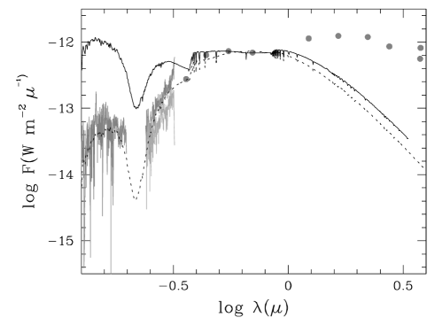
Figure 9: The observed spectral energy distribution of VV Ser (grey lines and dots) and two fits to its photospheric SED. The black dotted line (shown as a solid line in the upper-right panel of Fig. 8) corresponds to a Kurucz model with $T_{\rm eff}\!=\!14000$ K, $\log g_{*}\!=\!4.0$ reddened with the extinction law with $R_{V}\!=\!3.1$ and $E(B-V)=1.10$. The black solid line is the same Kurucz model reddened with with $E(B-V)=0.80$ but using the extinction law with $R_{V}\!=\!5.0$ (see text for details).

VV Ser is the star in the sample for which a larger amount of extinction was needed to reasonably fit the photospheric SED. In subsection 4.1 we mentioned that the total-to-selective extinction $R_{V}\!=\!3.1$ was used instead of a larger value ($R_{V}\!\sim\!5$) suggested by some studies that could be more appropriate to treat the environment of HAeBe stars (Hernández et al. 2004). Figure 9 shows the SED of VV Ser plotted in the same way as in Fig. 8 (upper panels). The black dotted line represents the Kurucz model with $T_{\rm eff}\!=\!14000$ K, $\log g_{*}\!=\!4.0$ reddened with the extinction law with $R_{V}\!=\!3.1$ and $E(B-V)=1.10$ (also shown in Fig. 8, upper-right panel) whereas the black solid line represents the same Kurucz model, reddened with $E(B-V)=0.80$ but using the extinction law with $R_{V}\!=\!5.0$; the parametrization given by Cardelli et al. (1989) has been used. Whereas the results of the SED fitting are roughly comparable and acceptable for both values of $R_{V}$ for the optical and near-IR parts of the SED, the ultraviolet part cannot be fitted with the $R_{V}\!=\!5.0$ law; if one attempts to fit the ultraviolet part, the amount of extinction needed is such that it is impossible to fit at the same time the UV and the optical and near-IR intervals. Since the extinction law with $R_{V}\!=\!3.1$ allows us to treat consistently the range of wavelengths from UV to the near-IR, that value of $R_{V}$ was considered the most appropriate for the analysis. The extinctions needed to fit the SEDs of the remaining stars are lower than for VV Ser, therefore we decided to use the same law for all the objects, giving an homogeneous treatment to the whole sample.

6.4.2 RR Tau

This object is a highly variable HAeBe star also classified as UXOR-type (Thé et al. 1994; Oudmaijer et al. 2001; Rodgers et al. 2002). The determination of its absolute parameters is very difficult because the variability observed does not allow to discern clearly what properties remain unchanged, and hence can be attributable to the –non-variable– stellar photosphere, and what are totally due to the presence of circumstellar material passing in front of the star.

Fig. 10 shows the SED of this system from the ultraviolet to the infrared, plotted in the same way as we did for VV Ser in the previous paragraph. Given the high degree of variability of this star and the different epochs when the ultraviolet IUE spectra and the optical photometry were obtained, it is not trivial to compare both sets of observations. A simple way, accurate enough for the purpose of this analysis, is to scale the ultraviolet observations to the UBVRI points according to the value of V in both epochs. The ultraviolet spectra shown in the figure were obtained between JD 2449268.446 and 2449268.622 (mean JD 2449268.534). We have found in the AAVSO archives that $V\!=\!12.3$ on JD 2449268.4 and $V\!=\!11.8$ on JD 2449269.4, with the brightness increasing the adjacent two days. An interpolation between the magnitudes on the mentioned dates and JD 2449268.534 gives $V\!=\!12.2$ for the moment when the IUE observations were obtained. Since $V\!=\!10.92$ when the optical photometry was taken, we have shifted the ultraviolet spectra upwards by 0.512 dex to make comparable both sets of observations. The best fit to this SED is obtained with a Kurucz model with $T_{\rm eff}\!=\!10000$ K, $\log g_{*}\!=\!3.5$, reddened with $E(\!B-\!V)\!=\!0.50$.

The value of the gravity deduced for this effective temperature by using the Balmer profiles is $\log g_{*}\!=\!3.31\pm 0.13$, which implies the following set of parameters: $M_{*}\!=\!5.79^{-0.94}_{+0.99}$ $M_{\odot}$, $L_{*}\!=\!780.5^{-351.9}_{+446.7}$ $L_{\odot}$, Age=0.4${}^{+0.3}_{-0.2}$ Myr and, after combining the luminosity and the observed flux, a distance $d\!=\!2103^{-544}_{+535}$ pc. Note that the age is fairly low to be in agreement with the evolutionary scenario desribed by Malfait et al. (1998). The value of the distance implied by this solution seems to be quite large compared with estimates done for this star, which place the object at around 800 pc (Finkenzeller & Mundt, 1984). As it happened with the low effective temperature case for VV Ser, the solution found for RR Tau could be made compatible with that value of the distance if a fraction $\alpha\!=\!0.86$ of the stellar light were completely blocked by the disk. The classification of RR Tau as an UXOR star would favour a moderate-to-high inclination for the disk, justifying this assumption.

Looking for a solution with a higher effective temperature, we have explored the accuracy of the fits between the SED and the models of a grid with effective temperatures from 11000 to 14000 K (steps of 1000 K), reddened with colour excesses $E(B\!-\!V)$ from 0.50 to 0.90. In opposition to what happened in the case of VV Ser, we have not found a solution that fits reasonably well the observed SED, therefore we have adopted for RR Tau the effective temperature, gravity and stellar parameters shown in Tables 2 and 3. Our results are consistent with those reported by Grinin et al. (2001; $T_{\rm eff}\!=\!9750$ K, $\log g_{*}\!=\!3.5$, solar metalicity) and Rodgers et al. (2002; 9000 $\leq T_{\rm eff}\leq$ 10000, 3.0 $\leq\log g_{*}\leq$ 3.5).

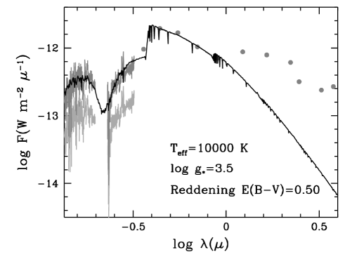
Figure 10: The observed spectral energy distribution of RR Tau (grey lines and dots) and the fit to the photospheric contribution (black line). The UV spectra were obtained with the International Ultraviolet Explorer (IUE); in light grey lines the spectra SWP 48866 (7/10/1993)) and a merge of LWP 26522 and LWP 26254 (7–8/10/1993) are plotted. Taking into account the value of the $V$ magnitude in the epochs when the ultraviolet observations were obtained ($V\!=\!12.2$), and when the $UBVRI$ photometry (dark grey dots) was taken ($V\!=\!10.92$, 31/01/1999), the IUE spectra have been shifted upwards by 0.512 dex (dark grey lines) in order to make ‘comparable’ the observing conditions of the two epochs. The SED is fitted with a Kurucz model with $T_{\rm eff}\!=\!10000$ K, $\log g_{*}\!=\!3.5$, reddened with $E(\!B-\!V)\!=\!0.50$.

6.4.3 HR 26 A, HR 4757 A and HR 5422 A

These three stars were included in the sample as hot companions of post-T Tauri stars, extracted from the Lindroos catalogue (Lindroos, 1985). Gerbaldi et al. (2001) carried out a systematic study of a sample binary systems with post-T Tauri secondaries. Both components, A and B, of HR 26 (HD 560), HR 4757 (HD 108767) and HR 5422 (HD 127304) were analysed in detail in that work and effective temperatures, gravities, luminosities, masses and ages were computed. The effective temperatures and gravities were obtained by those authors from calibrations using both $ubvy\beta$ and Geneva photometry; the luminosities, masses and ages were estimated in a different way from that followed in this paper: using the Hipparcos parallax and the $V$ magnitude of each star, they computed $M_{\rm bol}$ and then $L_{*}/L_{\odot}$, placing the star in a $\log L_{*}/L_{\odot}-\log T_{\rm eff}$ HR diagram and from its position, the remaining parameters were derived.

Table 4: Some stellar parameters for HR 26, HR 4757 and HR 5422.

Star	$T_{\rm eff}$ (K)	$\log g_{*}$	Age (Myr)	Tracks
HR 26 A	11400	$4.14\pm 0.04$	$130^{-40}_{+47}$, $140^{-30}_{+64}$	1,2
HR 26 B			$20^{+13}_{-8}$, $30^{+70}_{-8}$	1,2
HR 4757 A	10400	$4.05\pm 0.06$	$200^{-30}_{+40}$, $200\pm 30$	1,2
HR 4757 B			$40_{-17}$, $90_{-50}$	3,4
HR 5422 A	10040	$4.12\pm 0.02$	$240^{-30}_{+60}$, $240^{-20}_{+60}$	3,4
HR 5422 B			$50_{-20}$, $100_{-50}$	3,4
HR 26 A	11400	$4.08\pm 0.05$	175${}^{-23}_{+14}$	5
			1.8${}^{+0.4}_{-0.2}$	6
HR 4757 A	10400	$4.06\pm 0.05$	260${}^{-24}_{+14}$	5
			2.5${}^{+0.5}_{-0.2}$	6
HR 5422 A	10250	$4.08\pm 0.06$	267${}^{-39}_{+23}$	5
			2.1${}^{+0.1}_{-0.4}$	6

Notes to Table 4: The results shown in the upper part of the table are from Gerbaldi et al. (2001), those in the lower part are derived in this work. The tracks used for computing the ages are: ¹Schaller et al. (1993), ²Girardi et al. (2000), ³D’Antona & Mazzitelli, I. (1998), ⁴Palla & Stahler (1999), ⁵Y² post-MS, ⁶Y² PMS.

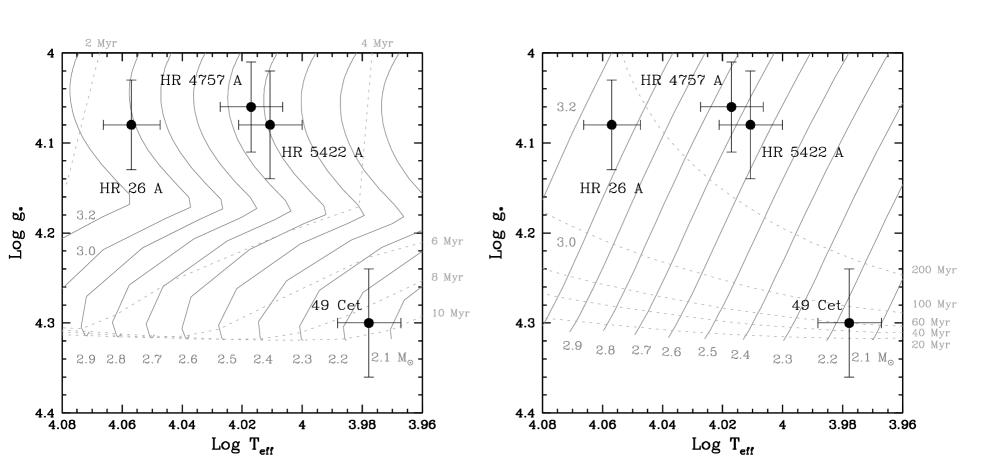
Figure 11: Two HR diagrams $\log g_{*}-\log T_{\rm eff}$ where the positions of the stars HR 26 A, HR 4757 A, HR 5422 A and 49 Cet have been plotted. The error bars in $\log T_{\rm eff}$ correspond to uncertainties of $\pm 250$ K. The diagrams show the stars plotted on PMS (left) and post-MS (right) tracks (solid lines) and isochrones (dashed lines) for solar metallicity from Yi et al. (2001).

Table 4 shows a comparison of the results from Gerbaldi et al.’ work and ours. The results shown in the upper part are extracted from Tables 1 (effective temperatures and gravities), 7 and 9 (ages of the early and late-type stars, respectively) of Gerbaldi et al. (2001); those in the lower part are from Tables 2 and 3 of this work. For the late-type stars we just list the ages found by Gerbaldi et al. (2001) in order to have all data needed for the discussion of the results.

One should not be confused with the terminology ‘hot companion of a post-T Tauri star’ attributed to these stars in the sense of assuming as a real fact that they are physically linked to the late-type companion. Gerbaldi et al. (2001) came to the conclusion that for HR 26, the ages of the components were compatible with a physical association between them due to the overlap of the error bars of the ages. The lack of that overlap lead these authors to conclude that the components of HR 4757 and HR 5422 are not linked (see Table 4). Note, however, that the result on HR 26 hinges on a large error in the determination of the age of the late-type star, therefore, in our opinion, that claim is very uncertain.

Strictly speaking, only with the data corresponding to the effective temperature and gravity (or luminosity), it is impossible to say whether these three stars are in a PMS or a post-MS evolutionary stage. When the corresponding points ($\log T_{\rm eff}$, $\log g_{*}$) –or ($\log T_{\rm eff}$, $\log L_{*}/L_{\odot}$), if the $V$ magnitudes, bolometric corrections and Hipparcos distances are used– are placed in the HR diagram, they lie above the main sequence. In Figure 11 we can see two HR diagrams, on the left we have plotted our results on the Y² tracks and isochrones for PMS stars and on the right, on the Y² set for the post-MS. In Tables 3 and 4 we give the results derived for both cases. The PMS ages are small, less than 3 Myr in all cases, whereas the post-MS ages are in the range 150-300 Myr, consistent with the results by Gerbaldi et al., although slightly larger.

The SEDs do not show any remarkable infrared excess: HR 26 A and HR 5422 A do not have IRAS detections, and HR 4757 A has IRAS fluxes at 12 and 25 $\mu$m lying slightly above the photospheric continuum and only upper limits at 60 and 100 $\mu$m. HR 26 A has a detection at 1.3 mm above the photospheric continuum (Altenhoff et al., 1994). However, the absence of an infrared excesses cannot, in principle, rule out the results extracted from PMS tracks, since it is not guaranteed that all A-type PMS stars in the age range 1-10 Myr have large infrared excesses indicating the presence of a circumstellar disk. None of the stars show H$\alpha$ in emission.

Pallavicini et al. (1992) carried out optical spectroscopy of post-T Tauri star candidates. HR 26 B (G5 Ve) and HR 4757 B (K2 Ve) show strong Ca ii emissions and Li absorptions, which are indications of youth, whereas HR 5422 B (K1 V) does not have Ca ii emission and the Li absorption is weak, which implies that this object must be older than the other two stars. The ages derived by Gerbaldi et al. for the ‘B’ components, listed in Table 4, are consistent with those observations, but in all cases they are larger (under the assumption that the ‘A’ components are PMS objects) or smaller (assuming that the ‘A’ components are post-MS stars), by very significant differences, than the ages of the corresponding early-type companions. Therefore, we can conclude that in none of the three cases the pairs are physically linked.

6.4.4 49 Cet and other stars without H$\alpha$ emission

In Table 1 we indicate what stars show the H$\alpha$ line in emission. It is well known that stars without disks with effective temperatures in the range of those considered in this work show the H$\alpha$ line –and all the lines of the Balmer series– in absorption. The presence of emission in PMS stars with protoplanetary disks is an indication of winds (Finkenzeller & Mundt, 1984), accretion (e.g. Muzerolle et al. 2005), or a combination of both (Kurosawa et al. 2006). Since the typical lifetime of protoplanetary disks is a few million years (Alexander, 2007), these phenomena are an indication of youth, and therefore the status of PMS assumed a priori for all the stars in our sample with H$\alpha$ emission is coherent.

However, the fact that a star does not show H$\alpha$ in emission does not imply, in principle, that the object has abandonned the PMS phase. In our sample there are stars with no emission but showing remarkable infrared excesses, indicative of the presence of a disk.

The case of 49 Cet is especially interesting. The peculiarity of this object is that its disk has retained a substantial amount of molecular gas, which is a typical feature of protoplanetary disks (i.e. ages less than $\sim\!10$ Myr) but shows dust properties similar to those of debris disks (Hughes et al. 2008). The spectrum, as can be seen in Fig. 5, is purely photospheric, and does not show any signature of circumstellar activity.

In Table 3 we give the stellar parameters for this object using both PMS and post-MS tracks and isochrones. Fig. 11 shows the position of the star in two HR diagrams; on the left, the Y² PMS tracks and isochrones have been used, on the right, the post-MS set has been plotted. Thi et al. (2001) assigned an age of 7.8 Myr to 49 Cet using PMS tracks, which is in good agreement with our PMS determination. Our estimations of the effective temperature and gravity place the star almost on the main sequence, therefore its evolutionary status can be that of a star either on the PMS phase, entering the MS, or just evolving out of it. Actually, the uncertainties in the gravity are such that they allow the star to be exactly on the main sequence.

The region of the HR diagram where 49 Cet lies is particularly difficult to carry out an estimation of ages: the isochrones are very close to each other and therefore a small change in gravity implies a large change in age. In the case of this star, the range of ages covered assuming that the star is in a PMS phase or in a post-MS stage is 8.9–61 Myr, hence any age in between these two determinations could be a reasonable result. Hughes et al. (2008) suggest that the disk might be in an unusual transitional phase and our results are in agreement with this hypothesis.

As it can be seen in Table 1, in addition to HR 26 A, HR 4757 A and HR 5422 A, already studied in the previous subsection, there are other stars without H$\alpha$ emission. Those objects have been classified as A-shell or Vega-like stars, implying that the corresponding infrared excesses are not very large. However, these stars deserve further and more detailed study since the ages derived from PMS tracks (see Table 3) are in all cases less than 6 Myr and some objects, e.g. HR 10 and $\lambda$ Boo show a high degree of circumstellar activity.

7 Final remarks

Effective temperatures, gravities, metallicities, masses, luminosities, ages and distances (or upper limits), have been obtained for a sample of 30 early-type objects, more precisely 27 HAeBe, Vega-type and Ash stars, and three hot –suspected and finally ruled out– companions of post-T Tauri stars. The results obtained are described in detail in Section 5 and discussed in Section 6.

As a bottom line of this paper we would like to stress the difficulty of finding the correct stellar parameters for this kind of objects. As we have seen in the cases of VV Ser and RR Tau, shown in subsection 6.4, the spectral energy distributions are difficult to interpret and the assumption that the ultraviolet, optical and near infrared parts of the SED originate entirely in the photosphere must be assessed in each case. Simultaneity of the observations in all wavelength ranges is crucial to build a consistent SED; in this work we have used ultraviolet data that were obtained long before the optical and near infrared data, this must be always be present in the analysis of the SED. Also, the wings of the Balmer lines used to compute the gravity are supposed to be purely photospheric, without any external contamination. Note that these hypotheses, underlying the whole procedure, are the starting points to determine the remaining set of stellar parameters. The extinction caused by the environment and the variability of the objects can also mask the ‘true photosphere’, if that concept is applicable to this kind of stars.

On the other hand, the uncertainties in the determination of temperatures and gravities put a limit to the accuracy of the ages estimated using isochrones. As it can be seen in Figs. 6 and 11, depending on the region of the HR diagram where a given star lies, the shape and position of the isochrones provides in some cases a wide range of ages. In particular, when the star lies very near the main sequence, as it happens to 49 Cet, even the determination of the evolutionary status as PMS or post-MS object can be a problem.

In view of these considerations we suggest to take the ages found in this paper –and in general, all the determinations of ages at this evolutionary stage using isochrones– with caution, assessing each particular case in a critical way and complementing their values with those of an observable quantity, such as $F_{\rm IR}/F_{*}$, i.e. the ratio between the excess flux from the disk and the photospheric flux, which can be taken as a proxy for the age of the system.

We would also like to remark that the method proposed to obtain the stellar parameters is distance-independent, in the sense that it is based on the determination of the effective temperature and gravity, which are used, via a transformation from a $\log g_{*}-\log T_{\rm eff}$ HR diagram into a $\log L_{*}/L_{\odot}-\log T_{\rm eff}$ HR diagram, to compute the remaining parameters. The method has proven to be reliable, given the agreement between the distances found in this work and those available from Hipparcos measurements (see subsection 6.3 and Fig. 7). For those stars with unknown distances, our determinations are upper limits to the real values.

The tasks carried out in this paper, resulting in the characterization of the stars, are necessary steps to study and model their circumstellar disks. Work is already in progress to show a global picture of the behaviour of the disks of these stars and their interaction, via accretion processes, with the star.

Appendix A

In this Appendix we treat the problem of how to compute a meaningful ‘mean metal abundance’ from measurements of individual elemental abundances. Let us consider the case of a set of elemental abundances, some of which have been obtained using lines of two different ionization stages.

Let $x_{i}(j)$ be the elemental abundance of the element $i$ obtained using absorption lines of its $j$-th ionization stage, i.e. $x_{i}(j)=[{\rm A}_{i}(j)/{\rm H}]$ and let $\Delta x_{i}(j)$ be the corresponding error.

In the particular case when an element has different measurements of the abundances using lines of two ionization stages, namely I and II, we obtain the abundance of that element by averaging the individual values weighted by a factor equal to the inverse of the square of their errors:

$$x_{i}=[{\rm A}_{i}/{\rm H}]=\frac{x_{i}({\rm I})/\Delta^{2}x_{i}({\rm I})+x_{i}({\rm II})/\Delta^{2}x_{i}({\rm II})}{1/\Delta^{2}x_{i}({\rm I})+1/\Delta^{2}x_{i}({\rm II})}$$ (1)

and

$$\Delta^{2}x_{i}=\sigma^{2}=\frac{1}{1/\Delta^{2}x_{i}({\rm I})+1/\Delta^{2}x_{i}({\rm II})}$$ (2)

In this way, if the measurement from one ionization state is much more precise than the other, the average value and its error will approach the best ones. However, if both measurements have equal precision, the average error will be reduced by a factor $\sqrt{2}$.

Once we have all the elemental abundances and their errors, i.e. the pairs $x_{i}$, $\Delta x_{i}$, we can proceed with the calculation of the mean metal abundance:

Let $B_{i}$ be

$$B_{i}=\left(\frac{N_{\rm A_{i}}}{N_{\rm H}}\right)_{\odot}$$ (3)

The mean metallicity can be computed as:

$${\rm[M/H]}=\log\sum_{i}B_{i}\,10^{x_{i}}-\log\sum_{i}B_{i}$$ (4)

where the sums extended over all $i$ metallic elements. Since only a few metallicities are measurable for each star, the sum will be restricted to those atoms, assuming that the remaining unknown abundances will not alter significantly the result.

The error in the determination of the mean abundance can be treated as follows: since ${\rm[M/H]}=f(x_{1},\dots,x_{N})$ then

$$\sigma({\rm[M/H]})=\sqrt{\sum_{i}\left(\frac{\partial f}{\partial x_{i}}\Delta x_{i}\right)^{2}}$$ (5)

where

$$\frac{\partial f}{\partial x_{i}}=\frac{B_{i}\,10^{x_{i}}}{\sum_{j}B_{j}\,10^{x_{j}}}$$ (6)

according to equation (4).

Acke & Waelkens (2004) provide the values of [A_i/H] and use the solar abundances by Anders & Grevesse (1989), so in principle, it is not difficult to compute an average abundance to be compared with ours. The problem, however is a bit more subtle and a direct comparison is not as trivial as it may appear. Acke & Waelkens (2004) divide the results in three tables: their table 2 contains the C, N, O and S abundances; table 3 contains the abundances of ‘metals’, where by ‘metals’ they mean Mg, Si, Ca, Ti, Fe and Sr, and finally table 4 contains the abundances of other elements, namely Na, Al, Sc, V, Cr, Mn, Ni, Zn, Y, Zr and Ba.

Table 5: Mean abundances for the sample of Acke & Waelkens (2004).

Star	Metals	[Fe/H]
HD 4881	$-0.78\pm 0.05$	$-0.64\pm 0.09$
HD 6028	$-0.18\pm 0.06$	$-0.13\pm 0.01$
HD 17081	$-0.09\pm 0.13$	$-0.26\pm 0.19$
HD 17206	$-0.07\pm 0.05$	$-0.09\pm 0.11$
HD 18256	$+0.06\pm 0.03$	$+0.06\pm 0.11$
HD 20010	$-0.17\pm 0.05$	$-0.16\pm 0.12$
HD 28978	$\,0.00\pm 0.08$	$+0.18\pm 0.11$
HD 31293	$-0.35\pm 0.03$	$-1.04\pm 0.12$
HD 31648	$+0.33\pm 0.08$	$+0.07\pm 0.10$
HD 33564	$+0.14\pm 0.03$	$-0.38\pm 0.13$
HD 36112	$-0.02\pm 0.07$	$-0.14\pm 0.08$
HD 95418	$+0.07\pm 0.04$	$+0.23\pm 0.06$
HD 97048	$-0.75\pm 0.06$	$-$
HD 97633	$+0.08\pm 0.08$	$+0.01\pm 0.08$
HD 100453	$+0.03\pm 0.05$	$-0.09\pm 0.13$
HD 100546	$-1.05\pm 0.08$	$-1.30\pm 0.13$
HD 102647	$-0.19\pm 0.08$	$-0.21\pm 0.09$
HD 104237	$+0.06\pm 0.05$	$+0.09\pm 0.12$
HD 135344	$+0.01\pm 0.07$	$-0.08\pm 0.10$
HD 139614	$-0.32\pm 0.04$	$-0.27\pm 0.11$
HD 190073	$+0.02\pm 0.05$	$-0.04\pm 0.10$
HD 244604	$-$	$-0.25$
HD 250550	$-0.40\pm 0.06$	$-0.88\pm 0.12$

Instead of computing the mean metallicity using all the elemental abundances, the criterion we have chosen is to include only abundances of the ‘metals’. These averages, and their uncertainties, are shown in the second column of Table 5. The reason for this is that, since the atomic fractions of C, N, O and S are much larger than those of the remaining elements, these four elements would dominate the whole mean value. As the optical spectrum of early-type stars is dominated by lines of ‘metals’, the abundances we have computed for the stars in our sample are, in fact, related to to those species and not to the lighter elements, namely, C, N, O and S.

For comparison we give in the third column of Table 5 the Fe abundances. Note that they can be quite different from the mean abundances obtained from the metals. This comes from the fact that the elemental abundance ratios in these stars differ in general from the solar ones, so the abundances of other ‘metals’, mainly Mg and Si, have a strong weight on the mean abundance.