The outer regions of galaxy clusters:
Chandra constraints on the X-ray surface brightness

Abstract

Context. We study the properties of the X-ray surface brightness profiles in a sample of galaxy clusters that were observed with Chandra and have emission detectable with a signal-to-noise ratio higher than 2 per radial bin at a radius beyond $R_{500}\approx 0.7\times R_{200}$.

Aims. Our study aims to measure the slopes in both the X-ray surface brightness and gas density profiles in the outskirts of massive clusters. These constraints are compared with similar results obtained from observations and numerical simulations of the temperature and dark-matter density profiles with the intention of presenting a consistent picture of the outer regions of galaxy clusters.

Methods. We extract the surface brightness profiles $S_{b}(r)$ of 52 X-ray luminous galaxy clusters at $z>0.3$ from X-ray exposures obtained with Chandra. These objects, which are of both high X-ray surface brightness and high redshift, allow us to use Chandra either in ACIS-I or even ACIS-S configuration to survey the cluster outskirts. We estimate $R_{200}$ using both a $\beta-$model that reproduces the surface brightness profiles and scaling relations from the literature. The two methods converge to comparable values. We determine the radius, $R_{S2N}$, at which the signal-to-noise ratio is higher than 2, and select the objects in the sample that satisfy the criterion $R_{S2N}/R_{200}>0.7$. For the eleven selected objects, we model by a power-law function the behaviour of $S_{b}(r)$ to estimate the slope at several characteristic radii expressed as a fraction of $R_{200}$.

Results. We measure a consistent steepening of the $S_{b}(r)$ profile moving outward from $0.4R_{200}$, where an average slope of $-3.6$ ($\sigma=0.8$) is estimated. At $R_{200}$, we evaluate a slope of $-4.3$ ($\sigma=0.9$) that implies a slope in the gas density profile of $\approx-2.6$ and a predicted mean value of the surface brightness in the $0.5-2$ keV band of $2\times 10^{-12}$ erg s^-1 cm^-2 deg^-2.

Conclusions. Combined with estimates of the outer slope of the gas temperature profile and expectations about the dark matter distribution, these measurements lie well within the physically allowed regions, allowing us to describe properly how X-ray luminous clusters behave out to the virial radius.

1 Introduction

Galaxy clusters form by the hierarchical accretion of cosmic matter. The end products of this process are virialized structures that, in the X-ray band, exhibit similar radial profiles of surface brightness (e.g. Vikhlinin et al. 1999, Neumann 2005), plasma temperature (e.g. Allen et al. 2001, Vikhlinin et al. 2005) and dark matter distribution (e.g. Pointecouteau, Arnaud & Pratt 2005). These measurements have been improved due to the arcsec resolution and large collecting area of the X-ray satellites, such as Chandra and XMM-Newton, but still remain difficult because of the high signal-to-noise ratio required. On the other hand, the X-ray surface brightness is a far easier quantity to observe and define, which is rich in physical information being proportional to the emission measure of the emitting source. Recent work focused on a few local bright objects with ROSAT PSPC observations, which have low instrumental background and large field of view, to recover and characterise the X-ray surface brightness profile over a significant fraction of the virial radius (Vikhlinin et al. 1999, Neumann 2005).

In this work, we study the X-ray emission of a sample of galaxy clusters in the redshift range $0.3-1.3$ observed with the arcsec resolution of Chandra (see Balestra et al. 2007), with the purpose of mapping, even at high redshift, a region out to $R_{200}$ and place reasonable constraints on the slope of the gas density in the outskirts of hot ($kT>3$ keV) galaxy clusters.

We assume a Hubble constant of 70 $h_{70}$ km s^-1 Mpc^-1 in a flat universe with $\Omega_{\rm m}$ equal to 0.3. All quoted errors are presented as the 1 sigma confidence level, unless otherwise stated.

2 Preparation of the dataset

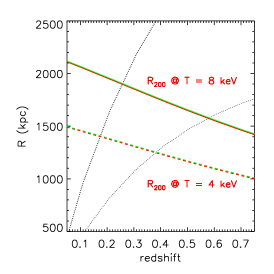
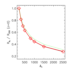
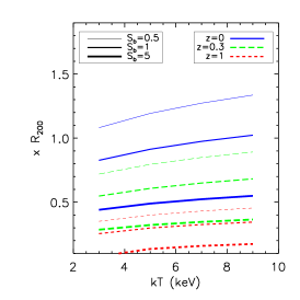
Figure 1: (Left) Expected $R_{200}$ for an object with 4 (dashed line) and 8 keV (solid line) and radius corresponding to 4 and 8 (thickest line) arcmin for the assumed $\Lambda$CDM cosmology as function of the observed redshift. Two estimates, almost indistinguishable, of $R_{200}$ are provided, one obtained with a $\beta-$model with core radius of 0.1 Mpc and $\beta=0.6$ (thickest lines), the other from the best-fit relation in Arnaud et al. (2005): $h_{z}R_{200}=1714(\pm 30)(T/5{\rm keV})^{0.50\pm 0.05}$. (Center) Fraction of $R_{200}$ mapped within a given overdensity $\Delta_{\rm c}$ at redshift $0$ for a cluster with a gas temperature of 4 (diamonds and dashed line) and 8 keV (solid line). The region at $\rho/\rho_{\rm c}=500$ is enclosed within a sphere with radius $\approx 0.65\times R_{200}$. The dotted line indicates the mapped fraction of $R_{200}$ assuming a Navarro-Frenk-White profile (e.g. Navarro et al. 2004) with concentration of 6, typical for the massive objects under consideration. (Right) Regions mapped (as fraction of $R_{200}$) for fixed surface brightness at different redshifts and gas temperatures, $S_{b}\sim T^{0.5}(1+z)^{-4}$. As reference, a value of $S_{b}=1$ at $R_{200}$, $z=0$, $kT=8$ keV and a $\beta-$model with core radius of 0.1 Mpc and $\beta=0.6$ are adopted.

Table 1: Sample of galaxy clusters, which satisfies the criterion $R_{S2N}/R_{200}>0.7$. The columns show: the name of the cluster, the observation IDs, in which ACIS configuration has been observed, the exposure time, the adopted X-ray center, the Galactic absorption from Dickey & Lockman (1990) in correspondence of the X-ray center, the redshift, the gas temperature, the mean local background, $B$, in counts observed in the $0.5-5$ keV band, and the average distance $D_{B}$ of the regions used to estimate the local background from the X-ray center. Note: MACSJ0744.9+3927 is the merger of three exposures with IDs 3197, 3585, and 6111.

cluster	Obs ID	ACIS	$t_{\rm exp}$	RA	Dec	$n_{H}$	$z$	$kT$	$B(\times 10^{-3})$	$D_{B}$
			ks	h m s	degree	$10^{20}$ cm-3		keV	cts/s/arcmin2	$R_{200}$
MS0015.9+1609	520	I	67.4	0 18 33.8	+16 26 12	4.1	0.541	$9.59\pm 0.43$	$1.61\pm 0.03$	$1.35$
MACSJ2228.5+2036	3285	I	19.9	22 28 33.9	+20 37 15	4.6	0.412	$8.25\pm 0.59$	$2.00\pm 0.07$	$0.92$
MACS0744.9+3927	Merged	I	89.0	7 44 52.8	+39 27 26	5.7	0.686	$9.58\pm 0.67$	$1.67\pm 0.04$	$1.64$
MACSJ0417.5-1154	3270	I	11.8	4 17 34.6	-11 54 33	3.9	0.440	$10.84\pm 0.98$	$2.33\pm 0.10$	$0.84$
RXJ1701.3+6414	547	I	49.5	17 01 23.8	+64 14 11	2.6	0.453	$4.36\pm 0.28$	$2.25\pm 0.05$	$1.18$
MACSJ1720.2+3536	3280	I	20.8	17 20 16.8	+35 36 26	3.4	0.391	$6.46\pm 0.33$	$1.87\pm 0.09$	$0.91$
RXJ1416.4+4446	541	I	28.5	14 16 27.8	+44 46 45	1.2	0.400	$3.43\pm 0.20$	$2.22\pm 0.06$	$1.38$
MACSJ2129.4-0741	3199	I	17.6	21 29 26.6	-7 41 29	4.8	0.570	$9.17\pm 0.90$	$1.88\pm 0.09$	$1.12$
MACSJ1621.3+3810	3254	I	9.8	16 21 24.9	+38 10 08	1.1	0.465	$6.62\pm 0.74$	$1.58\pm 0.10$	$1.21$
MS0451.6-0305	902	S	42.6	4 54 11.3	-3 00 56	5.0	0.540	$9.11\pm 0.45$	$3.98\pm 0.07$	$0.76$
MACSJ1206.2-0847	3277	I	23.4	12 06 12.1	-8 48 02	3.7	0.440	$11.98\pm 0.85$	$2.07\pm 0.06$	$0.78$

To study the outskirts of X-ray emitting galaxy clusters, possibly out to the virial region, we require bright objects located at an appropriate redshift to allow the Chandra field-of-view to encompass the interesting area. As shown in Fig. 1 (panel on the left) for a typical massive object, we should expect to resolve the region within an overdensity of 200, estimated with respect to the critical density at the cluster redshift, using instruments with a field-of-view of radius larger than 8 arcmin above redshift $0.2$. In the same figure, we plot the expected dependence of the radius (as a function of $R_{200}$) on both the cluster overdensity (central panel) and the gas temperature and redshift for a given surface brightness (panel on the right). These plots indicate that any overdensity is mapped within a fixed fraction of $R_{200}$ regardless of the cluster temperature and/or mass concentration (e.g. $\Delta_{\rm c}=500$ is reached at about $0.65R_{200}$ for any $T$ of interest, and with variations of 2 per cent with a concentration parameter in the range $4-8$ for a given Navarro-Frenk-White mass profile; e.g. Navarro et al. 2004), and the surface brightness that a galaxy cluster is expected to emit for a given $T$ and $z$ with respect to the value measured at $z=0$ in an object with $T=5$ keV (e.g. the same $S_{\rm b}$ value is expected in a 10 keV system at $z\sim 0.3$).

In the present work, we consider a sample of hot ($T_{\rm gas}>3$ keV), high-redshift ($0.3<z<1.3$) galaxy clusters described in Balestra et al. (2007). We refer to that work for details of the data reduction. We recall that the spectral analysis was performed by extracting the spectrum from a circular region of radius $\sim 0.15-0.3R_{200}$ defined in order to maximize the signal-to-noise ratio in each cluster. These regions contain the core emission, which has not been removed due to the low count statistics for the high redshift systems under consideration. On the other hand, results from observations and numerical simulations (e.g. Santos et al. 2008, Ettori & Brighenti 2008) indicate a lower incidence of cooling cores in clusters at higher redshift, suggesting that our overall estimates of $T_{\rm gas}$ should not be significantly biased towards low values. Moreover, the measurements of the gas temperature were used in our analysis only to infer a physical radius, which depends on the square root of $T_{\rm gas}$. Therefore, any error affecting our temperature estimates propagates only half of its value as a relative error on the physical radius of interest.

We prepare the exposure-corrected images in the energy band $0.5-5$ keV as described in Tozzi et al. (2003) and Ettori et al. (2004). The exposure maps for each cluster were computed by combining different instrumental maps at given energy, using weights defined from a thermal spectrum with the best-fit parameters obtained from our spectral analysis. The variations in the exposure map were not expected to be significant in the adopted energy band . We masked any detectable point sources with circular regions of radii large enough to include all the emission and, in any case, larger than 2 arcsec. We preferred to remove the point sources manually to avoid any possible confusion with detections by automatic algorithms (i.e. wavedetect) in proximity or within the extended emission of the clusters.

The center of the cluster was defined to correspond to the centroid of the raw image estimated in a box of width $\sim 10-20$ arcsec around the maximum of the image itself that had been smoothed with a moving average in a square box of width equal to $3-5$ arcsec.

The surface brightness profiles were extracted by requiring a fixed number of a minimum 50 counts per bin in the inner 10 radial bins and then collecting the counts within annulii for which the outer radius was increased at each step by a factor of 1.2.

A local background, $B$, was defined for each exposure by considering a region far from the X-ray center that covered a significant portion of the exposed CCD with negligible cluster emission. The estimated average value of $B$, its relative error, and the mean distance from the X-ray center of the region analysed to determine the background are quoted in Table 1.

We define the “signal-to-noise” ratio, $S2N$, to be the ratio of the observed surface brightness value in each radial bin, $S_{b}(r)$, after subtraction of the estimated background, $B$, to the Poissonian error in the evaluated surface brightness, $\epsilon_{b}(r)$, summed in quadrature with the error in the background, $\epsilon_{B}$: $S2N(r)=\left[S_{b}(r)-B\right]/\sqrt{\epsilon_{b}(r)^{2}+\epsilon_{B}^{2}}$. The outer radius at which the signal-to-noise ratio remained above $2$ was defined to be the limit of the extension of the detectable X-ray emission, $R_{S2N}$.

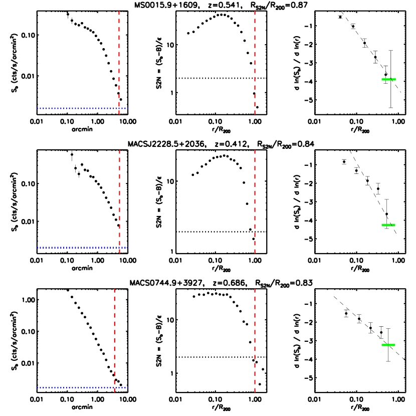
Figure 2: In the first column, we plot the surface brightness profiles of the objects under examination with the fitted background (horizontal dotted line) and the radius $R_{200}$ (vertical dashed line). The panels in the second column show the signal-to-noise profiles, evaluated as $S2N=(S_{b}-B)/\epsilon$, where the error $\epsilon$ is the sum in quadrature of the Poissonian error in the radial counts and the uncertainties in the fitted background, $B$. They are plotted as a function of $r/R_{200}$. In the third column, we plot the best-fit values of the slope of the surface brightness profiles as a function of $r/R_{200}$. These values are estimated over 6 radial bins. The thick horizontal solid line indicates the slope evaluated between $0.4\times R_{200}$ and $R_{S2N}$ with a minimum of 3 radial bins. The dashed line indicates the best-fit of $d\ln(S_{b})/d\ln(r/R_{200})$ with the functional form $s_{0}+s_{1}\ln(r/R_{200})$ over the radial range $0.1\times R_{200}-R_{S2N}$, with the best-fit parameters quoted in Table 3.

We note that the local background is about a factor of 2 higher in the ACIS-S field than in ACIS-I. We observe no significant correlation of $B$ with the Galactic absorption ($<6\times 10^{20}$ cm^-2 in the selected objects; a random deviation from the null value of no-correlation is expected with probability of $0.19$), indicating that we were dominated by cosmic and instrumental background. A negligible (with probability of $0.69$) correlation is also noticed between $B$ and the mean distance $D_{B}$ (see Table 1) of the region from which the local background is extracted. A slightly positive trend (significance of $1.6\times 10^{-4}$) was instead present between the estimated uncertainty $\epsilon_{B}$ and the exposure time of the observation, as expected.

To scale the radial quantity with respect to a physical radius, we estimated $R_{200}$ by using the single temperature measurement (see Table 1) and the best-fit description of $S_{b}(r)$ with a $\beta-$model (the best-fit parameters are shown in Table 2, obtained after fitting the background-subtracted profile over all positive values above 40 kpc) following the equation in Ettori (2000):

$$R_{200}=r_{\rm c}\times\left[\left(\frac{195.45\,\beta\,\gamma\,T_{\rm gas}}{\Delta_{\rm c}\,E_{z}^{2}\,h_{70}^{2}\,r_{\rm c}^{2}}\right)^{a}-1\right]^{0.5},$$ (1)

where $E_{z}=\left[\Omega_{\rm m}(1+z)^{3}+1-\Omega_{\rm m}\right]^{0.5}$, $\Delta_{\rm c}=200$, $a=\left[1.5\beta(\gamma-1)+1\right]^{-1}$, and the polytropic index $\gamma$ is fixed to be equal to 1.

Table 2: Best-fit results of the X-ray surface brightness profiles modelled with a $\beta-$model. $\overline{R_{200}}$ is estimated from the scaling laws in Arnaud et al. (2005); $R_{200}$ from Eq. 1; $R_{S2N}$ and $r_{\rm c}$ are quoted in unit of $R_{200}$.

cluster	$\overline{R_{200}}$	$R_{200}$	$R_{S2N}$	$r_{\rm c}$	$\beta$
	kpc	kpc	$R_{200}$	$R_{200}$
MS0015.9+1609	$1770$	$1948\pm 43$	$0.871$	$0.137\pm 0.005$	$0.742\pm 0.011$
MACSJ2228.5+2036	$1771$	$1743\pm 62$	$0.837$	$0.093\pm 0.007$	$0.587\pm 0.013$
MACS0744.9+3927	$1622$	$1566\pm 56$	$0.832$	$0.045\pm 0.003$	$0.561\pm 0.005$
MACSJ0417.5-1154	$1998$	$1936\pm 91$	$0.783$	$0.068\pm 0.006$	$0.567\pm 0.010$
RXJ1701.3+6414	$1258$	$1204\pm 44$	$0.731$	$0.087\pm 0.013$	$0.555\pm 0.020$
MACSJ1720.2+3536	$1587$	$1617\pm 42$	$0.726$	$0.056\pm 0.004$	$0.626\pm 0.012$
RXJ1416.4+4446	$1150$	$1133\pm 38$	$0.722$	$0.080\pm 0.010$	$0.587\pm 0.020$
MACSJ2129.4-0741	$1701$	$1684\pm 83$	$0.712$	$0.069\pm 0.006$	$0.592\pm 0.014$
MACSJ1621.3+3810	$1538$	$1516\pm 88$	$0.711$	$0.048\pm 0.007$	$0.585\pm 0.019$
MS0451.6-0305	$1727$	$1995\pm 52$	$0.705$	$0.118\pm 0.005$	$0.814\pm 0.015$
MACSJ1206.2-0847	$2100$	$2158\pm 77$	$0.703$	$0.067\pm 0.004$	$0.638\pm 0.009$

For comparison, we also estimated $R_{200}$ by adopting the scaling relation with $T_{\rm gas}$ obtained for massive clusters in Arnaud et al. (2005; similar results were presented in Vikhlinin et al. 2005): $\overline{R_{200}}=1714(\pm 30)\times(T_{\rm gas}/5{\rm keV})^{0.50\pm 0.05}h_{70}^{-1}E_{z}^{-1}$ kpc. The value of $\overline{R_{200}}$ was estimated and quoted in Table 2. No appreciable differences were present between the different estimates of $R_{200}$, such that the mean and standard deviation of the ratio of the two values were $1.02$ and $0.06$, respectively.

3 The surface brightness at $r>R_{500}$

We investigated the X-ray surface-brightness profiles of massive clusters at $r>R_{500}\approx 0.7R_{200}$ (see Fig. 1), selecting the 11 objects with $R_{S2N}/R_{200}>0.7$. The properties of these clusters are shown in Tables 1 and 2. Examples of the analysed dataset are shown in Fig. 2.

We performed a linear least-squares fit between the logarithmic values of the radial bins and the background-subtracted X-ray surface brightness, taking into account the data errors in both coordinates with the routine FITEXY (Press et al. 1992; as implemented in IDL).

The distribution of the error-weighted mean slopes above a fixed fraction of $R_{200}$ and within $R_{S2N}$ is shown in Fig. 3 and quoted in Table 3. Overall, the error-weighted mean slope is $-2.91$ (with a standard deviation in the distribution of $0.46$) at $r>0.2R_{200}$ and $-3.59(0.75)$ at $r>0.4R_{200}$. For the only 3 objects for which a fit between $0.5R_{200}$ and $R_{S2N}$ was possible, we measured a further steepening of the profiles, with a mean slope of $-4.43$ and a standard deviation of $0.83$.

We also fitted linearly the derivative (from numerical differentiation using three-point Lagrangian interpolation as described in Hildebrand 1987 and implemented in the IDL function DERIV) of the logarithm $S_{b}(r)$ over the radial range $0.1R_{200}-R_{S2N}$, excluding in this way the influence of the core emission (see values $s_{0}$ and $s_{1}$ in Table 3). The average (and standard deviation $\sigma$) values of the extrapolated slopes are then $-3.15(0.46)$, $-3.86(0.70)$, and $-4.31(0.87)$ at $0.4R_{200}$, $0.7R_{200}$ and $R_{200}$, respectively.

These values are comparable to these obtained in previous analyses. Vikhlinin et al. (1999) found that a $\beta-$model with $\beta=0.65-0.85$ described the surface brightness profiles in the range $0.3-1R_{180}$ of 39 massive local galaxy clusters observed with ROSAT PSPC. These values translate in a range of the estimate of the power-law slope ($-2.9/-4.1$, from $S_{b}(r)\approx r^{2(0.5-3\beta)}=r^{1-6\beta}$) that includes our estimates.

Neumann (2005) found that the stacked profiles of a few massive nearby systems located in regions of low ($<6\times 10^{20}$ cm^-3) Galactic absorption observed by ROSAT PSPC still provided values of $\beta$ around $0.8$ at $R_{200}$, with a power-law slope that increased from $-3$, when the fit was done over the radial range $[0.1,1]R_{200}$, to $-5.7^{+1.5}_{-1.2}$ over $[0.7,1.2]R_{200}$.

These observational results were supported by hydrodynamical simulations of X-ray emitting galaxy clusters performed with the Tree+SPH code GADGET-2 from Roncarelli et al. (2006). In the most massive systems, they measured a steepening of $S_{b}(r)$, independently from the physics adopted in treating the baryonic mass, with a slope of $-4,-4.5,$ and $-5.2$ when estimated for the radial range $0.3-1.2R_{200}$, $0.7-1.2R_{200}$, and $1.2-2.7R_{200}$, respectively. In particular, we note the good agreement between the slope of the simulated surface brightness profile of the representative massive cluster in the radial bin $0.7-1.2R_{200}$ (see values of $b_{A}$ in Table 4 of Roncarelli et al. (2006), ranging between $-4.29$ and $-4.54$) and our mean extrapolated value at $R_{200}$ of $-4.31$.

In Table 3, we quote the estimated surface brightness value at $R_{200}$ in CGS units. They were obtained by extrapolating the measured $S_{\rm b}$ at $\sim 0.7R_{200}$ out to $R_{200}$ by using the best-fit values quoted in the same Table. The conversion from the count rate to the flux was completed by adopting an absorbed thermal component at the cluster redshift with an assumed metallicity and temperature equal to (i) the ones measured and (ii) one third of the measured values. We predict an average surface brightness of about $2\times 10^{-12}$ erg s^-1 cm^-2 deg^-2 in the $0.5-2$ keV band, corresponding to about half of the value associated with the total cosmic background observed (e.g. Hickox & Markevitch 2006) and consistent with the estimates measured in the hydrodynamical simulations of massive galaxy clusters (Roncarelli et al. 2006). Converting this surface brightness to counts in the $0.5-5$ keV band, we predict that at $R_{200}$ the X-ray emission from a cluster is responsible of $\sim 5$ per cent of the total counts observable with Chandra.

Table 3: Best-fit values of the slope of the surface brightness profile in the radial range $[0.2\times R_{200},R_{S2N}]$ and $[0.4\times R_{200},R_{S2N}]$. The best-fit results of the first derivative of $S_{b}(r)$ over the entire radial range are indicated as $d\ln(S_{b})/d\ln(r/R_{200})=s_{0}+s_{1}\ln(r/R_{200})$ and shown in Fig. 2. The predicted slopes from the best-fit results at $0.4,0.7$, and $1\times R_{200}$ are quoted. In the last two columns, we present the expected surface brightness in the $0.5-2$ keV band and the fraction $fc_{200}$ of the clusters counts with respect to the total count rate measured in the $0.5-5$ keV at $R_{200}$.

cluster		slope			$(s_{0},s_{1})$	$0.4R_{200}$	$0.7R_{200}$	$R_{200}$	$S_{\rm b}(R_{200})$	$fc_{200}$
		$0.2R_{200}-R_{S2N}$	$0.4R_{200}-R_{S2N}$						$10^{-12}$ erg/s/cm2/deg2
MS0015.9+1609		$-3.30\pm 0.28$	$-3.89\pm 0.96$		$(-4.41,-1.33)$	$-3.19$	$-3.93$	$-4.41$	$(1.7,1.7)$	$0.051$
MACSJ2228.5+2036		$-2.74\pm 0.29$	$-4.26\pm 1.23$		$(-4.92,-1.75)$	$-3.32$	$-4.30$	$-4.92$	$(2.6,2.7)$	$0.057$
MACS0744.9+3927		$-2.73\pm 0.31$	$-3.23\pm 0.89$		$(-3.73,-0.88)$	$-2.92$	$-3.41$	$-3.73$	$(2.6,2.7)$	$0.074$
MACSJ0417.5-1154		$-3.38\pm 0.42$	$-4.53\pm 1.27$		$(-5.60,-2.02)$	$-3.75$	$-4.88$	$-5.60$	$(1.6,1.6)$	$0.034$
RXJ1701.3+6414		$-2.39\pm 0.27$	$-2.59\pm 1.17$		$(-4.24,-1.60)$	$-2.78$	$-3.67$	$-4.24$	$(2.4,2.6)$	$0.051$
MACSJ1720.2+3536		$-3.19\pm 0.36$	$-2.40\pm 1.32$		$(-3.57,-0.77)$	$-2.87$	$-3.30$	$-3.57$	$(2.5,2.6)$	$0.059$
RXJ1416.4+4446		$-2.74\pm 0.37$	$-3.63\pm 1.72$		$(-3.75,-0.94)$	$-2.89$	$-3.41$	$-3.75$	$(1.8,1.9)$	$0.042$
MACSJ2129.4-0741		$-2.68\pm 0.33$	$-4.16\pm 1.74$		$(-3.92,-1.13)$	$-2.88$	$-3.51$	$-3.92$	$(2.4,2.5)$	$0.060$
MACSJ1621.3+3810		$-2.64\pm 0.37$	$-3.53\pm 1.76$		$(-2.99,-0.45)$	$-2.58$	$-2.83$	$-2.99$	$(3.0,3.2)$	$0.087$
MS0451.6-0305		$-3.94\pm 0.45$	$-4.77\pm 2.04$		$(-5.85,-1.91)$	$-4.11$	$-5.17$	$-5.85$	$(0.3,0.3)$	$0.006$
MACSJ1206.2-0847		$-3.24\pm 0.37$	$-3.67\pm 1.64$		$(-4.43,-1.16)$	$-3.37$	$-4.02$	$-4.43$	$(1.4,1.5)$	$0.032$
mean		$-2.91$	$-3.59$		$(-4.31,-1.27)$	$-3.15$	$-3.86$	$-4.31$	$(2.0,2.1)$	$0.050$
$\sigma$		$0.46$	$0.75$		$(0.87,0.50)$	$0.46$	$0.70$	$0.87$	$(0.8,0.8)$	$0.022$

Figure 3: Error-weighted mean and standard deviation of the distribution of the values of the slope of the surface brightness in the radial range $r-R_{S2N}$ plotted as a function of the inner radius $r$. The number of objects with at least 3 points considered for this estimate is indicated.

4 Physical properties of the outer cluster regions

We combine the measured slope of the surface brightness in the cluster outskirts with the predicted slopes of the gas temperature and dark matter profiles. We have demonstrated that the slope depends on the radius at which it is measured. Thus, we focus hereafter on the properties at $R_{200}$, by representing with power-laws the radial dependence of the gas density, $n_{\rm gas}$, temperature, $T_{\rm gas}$, and dark matter, $\rho_{\rm DM}$, profiles:

$$\left\{\begin{array}[]{l}n_{\rm gas}\propto r^{a}\\ T_{\rm gas}\propto r^{b}\\ \rho_{\rm DM}\propto r^{c}.\end{array}\right.$$ (2)

The surface brightness, $S_{b}$, is the integral along the line of sight of the square of the gas density and can be written, assuming spherical geometry, as

$$S_{b}=\int n_{\rm gas}^{2}\Lambda(T)dl\ \propto n_{\rm gas}^{2}\Lambda(T)r\ \propto r^{2a\ +1\ +0.2b},$$ (3)

where we consider the weak dependence ($T\propto r^{0.2b}$) on the gas temperature of the cooling function, $\Lambda(T)$, due to the limited energy band $\Delta E=[0.5,5]$ keV in which the images were considered and the gas temperatures under consideration (e.g. Ettori 2000).

Hydrostatic polytropic gas can be described by the relation $T_{\rm gas}\propto n_{\rm gas}^{\gamma-1}$, with a polytropic index $\gamma$ that relates the ratio of specific heats in a adiabatic gas and equals $5/3$ for a monoatomic ideal gas. If the intracluster gas is not entirely adiabatic, the polytropic index can be used as a fitting parameter to describe the relative behaviour of the gas temperature and density profile. In particular, if the thermal conduction is an efficient process, the gas tends to be isothermal and $\gamma=1$, whereas the entropy per atom will be constant if the thermal conduction is slow and the gas is well mixed. Moreover, when $\gamma>5/3$, the gas becomes convectively unstable and mixing occurs within several sound crossing times, which are in general quite short compared to the overall age of the cluster. Therefore, this “polytropic condition” requires that $1\leq\gamma\leq 5/3$ and translates into the request that

$$0\leq\frac{b}{a}\leq\frac{2}{3}.$$ (4)

Further constraints are provided by the integrated masses. The gas mass estimate, $M_{\rm gas}\approx\int n_{\rm gas}dV\ \propto r^{a+3}$, requires that

$$a+3>0.$$ (5)

The total gravitating mass can be expressed both as an integral of the dark matter profile over the cluster volume

$$M_{\rm grav}=\int\rho_{\rm DM}dV\ \propto r^{c+3},$$ (6)

and with the assumption of hydrostatic equilibrium between dark matter and spherically symmetric intracluster gas

$$M_{\rm hyd}\approx-r\ T\ \left(\frac{d\ln n_{\rm gas}}{d\ln r}+\frac{d\ln T_{\rm gas}}{d\ln r}\right)\propto-(a+b)\ r^{b+1}.$$ (7)

The request for a gravitational mass increasing radially implies that $c+3>0$ and $a+b<0$. Moreover, by equating the two definitions of the gravitational mass, we find that the exponents of the radial dependence must to satisfy the condition $c+3=b+1$, which directly relates the slope of the dark matter profile to that of the gas temperature profile.

Overall, these conditions can be summarized by the following inequalities among the indices of the assumed power-laws:

$$\left\{\begin{array}[]{l}0\leq\frac{b}{a}\leq\frac{2}{3}\\ a+3>0\\ c+3>0\\ a+b<0\\ c=b-2\end{array}\right.$$ (8)

We show in Fig. 4 the allowed regions in the $a-b-c$ plane.

It is worth noting that the permitted values shown in these plots also satisfy the requests that the sound-crossing time, $t_{SC}\propto T_{\rm gas}^{-1/2}r\approx r^{1-b/2}$, the cooling time, $t_{cool}\propto T_{\rm gas}^{1/2}n_{\rm gas}^{-1}\approx r^{b/2-a}$, and the equipartition time for Coulomb collisions, $t_{eq}\propto T_{\rm gas}^{3/2}n_{\rm gas}^{-1}\approx r^{3b/2-a}$, increase with radius in the cluster outskirts.

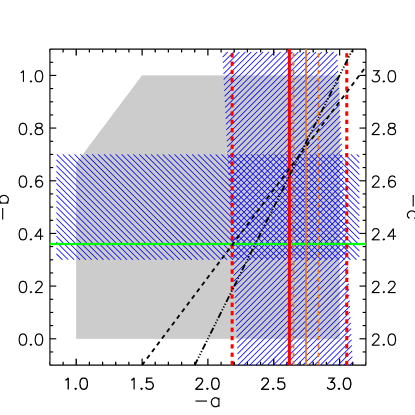
Figure 4: Constraints on the outer slopes of the gas density (index $a$), temperature (index $b$) and dark matter (index $c=b-2$) profiles. The shaded area shows the physically allowed regions for the index values as discussed in the text. The hatched regions indicate the $1\sigma$ constraints from Navarro et al. (2004; horizontal regions) and from the present work including the dependence upon the cooling function (vertical area). The horizontal green solid line shows the fiducial slope of the temperature profile from Vikhlinin et al. (2005). The vertical solid (and dashed) lines indicate the limits on the slope of the gas density profile from hydrodynamical simulations (tighter constraints in orange; Roncarelli et al. 2006) and from the present observational analysis (in red). The diagonal dashed line is the locus of the predicted behaviour of the entropy profile, $b-2a/3=1.1$. The dot-dot-dot-dashed line satisfies the condition that the gas fraction is constant in the cluster outskirts.

Some observational constraints are available and can be located in these graphs: (1) the mean value of the slope in the surface brightness at $R_{200}$ is $-4.31(\sigma=0.87)$, equal to $2a\ +\ 1\ +\ 0.2b$ as inferred by Eq. 3, and implies that $a=-2.62\pm 0.43$; (2) the dark matter profile behaves as $r^{-2.5\pm 0.2}$ as discussed and shown in Fig. 3 of Navarro et al. (2004); (3) a polytropic index $\gamma\approx 1.24$ is measured in the outskirts of temperature profiles (e.g. Markevitch et al. 1998, De Grandi & Molendi 2002 out to about $0.6R_{180}\sim 0.63R_{200}$; a value of $1.42\pm 0.03$ is estimated in one of the first spectral determination of the temperature profile at $R_{200}$, obtained for the cluster PKS0745-191 with Suzaku in George et al. 2008). These further constraints are also shown in Fig. 4.

The expected slope of the dark matter profile, combined with the observed slope in surface brightness, places constraints on the predicted behaviour of the temperature profile (Eq. 8) and its polytropic index, $\gamma=1+b/a$. For the values quoted above, we expect that $b\approx-0.5\pm 0.2$ and $\gamma\approx 1.19\pm 0.08$. These values agree well with the constraints obtained from observed data-sets (e.g. Markevitch et al. 1998, Vikhlinin et al. 2005, Leccardi & Molendi 2008, Reiprich et al. 2008, George et al. 2008), hydrodynamical simulated objects (e.g. Loken et al. 2002, Roncarelli et al. 2006) and analytical model of the ICM (e.g. Ostriker, Bode & Babul 2005).

Finally, the entropy profiles, $K(r)=T_{\rm gas}(r)/n_{\rm gas}^{2/3}$, both from smooth and hierarchical accretion models (e.g. Tozzi & Norman 2001, Voit 2005) are predicted to increase with radius as $K\propto r^{1.1}$. This shape of the entropy profile outside the core, but well within the virial radius, is also observed in high quality cluster exposures with the XMM-Newton satellite (Pratt & Arnaud 2003). By using our power-law expressions, we find that $K(r)\propto r^{b-2a/3}$, with a predicted value of the slope of $1.25\pm 0.35$ and $1.12$ for the simulated dark matter distribution and the observed polytropic index, respectively.

5 Summary and Conclusions

We have selected 11 massive galaxy clusters in the redshift range $0.3<z<0.7$ observed with Chandra, which is convenient to survey the X-ray emission out to a significant fraction of the virial radius and, in all the cases, to radii beyond $R_{500}\approx 0.65\times R_{200}$.

By fitting a single power-law function to the X-ray surface brightness profile $S_{b}(r)$ in different radial ranges, we have detected a consistent steepening in $S_{b}(r)$ moving outward, with a mean slope of $-2.9\pm 0.5$ when the radial range $0.2R_{200}-R_{S2N}$ is considered, and $-3.6$ (r.m.s. $0.8$) when the lower limit of the radial range is $0.4R_{200}$. The mean slope estimated from the linear fit to the derivative of $S_{b}(r)$ is $-3.2$, $-3.9$, and $-4.3$ at $0.4R_{200}$, $0.7R_{200}$, and $R_{200}$, respectively. These values, corrected by the weak dependence of the cooling function on gas temperature in the considered energy band $[0.5,5]$ keV, imply a slope in the gas density profile of $-2.04\pm 0.23$ ($\beta\approx 0.68$), $-2.39\pm 0.35$ ($\beta\approx 0.80$) and $-2.62\pm 0.43$ ($\beta\approx 0.87$) at $0.4R_{200}$, $0.7R_{200}$ and $R_{200}$, respectively.

Combined with previous estimates of the outer slope of the gas temperature profile (e.g. Vikhlinin et al. 2005, from an observational point of view; Roncarelli et al. 2006, for hydrodynamically simulated clusters) and the expectations for the dark matter distribution (e.g. Navarro et al. 2004), and modelling of the gas density, temperature and dark matter profiles with single power laws ($n_{\rm gas}\propto r^{a},T_{\rm gas}\propto r^{b},\rho_{\rm DM}\propto r^{c}$), we have defined a physically-allowed region in the $a-b-c$ plane, with a predicted behaviour at $R_{200}$ described by power-law indices of $a\approx-2.6,b\approx-0.5,$ and $c\approx-2.5$.

References

- (1) Allen S.W., Schmidt R.W., Fabian A.C., 2001, MNRAS, 328, L37
- (2) Arnaud M., Pointecouteau E., Pratt G.W., 2005, A&A, 441, 893
- (3) Balestra I., Tozzi P., Ettori S., Rosati P., Borgani S., Mainieri V., Norman C., Viola M., 2007, A&A, 462, 429
- (4) De Grandi S., Molendi S., 2002, ApJ, 567, 163
- (5) Dickey J.M., Lockman F.J., 1990, ARAA, 28, 215
- (6) Ettori S., 2000, MNRAS, 311, 313
- (7) Ettori S., Tozzi P., Borgani S., Rosati P., 2004, A&A, 417, 13
- (8) Ettori S., Brighenti F., 2008, MNRAS, 387, 631
- (9) George M.R., Fabian A.C., Sanders J.S., Young A.J., Russell H.R., 2008, MNRAS, submitted (arXiv:0807.1130)
- (10) Hickox R.C., Markevitch M., 2006, ApJ, 645, 95
- (11) Hildebrand F.B., 1987, Introduction to Numerical Analysis, Dover Publishing, New York, p.80
- (12) Leccardi A., Molendi S., 2008, A&A, 486, 359
- (13) Loken C., Norman M.L., Nelson E., Burns J., Bryan G.L., Motl P., 2002, ApJ, 579, 571
- (14) Markevitch M., Forman W.R., Sarazin C.L., Vikhlinin A., 1998, ApJ, 503, 77
- (15) Navarro J.F., Hayashi E., Power C., Jenkins A.R., Frenk C.S., White S.D.M., Springel V., Stadel J., Quinn T.R., 2004, MNRAS, 349, 1039
- (16) Neumann D.M., 2005, A&A, 439, 465
- (17) Ostriker J.P., Bode P., Babul A., 2005, ApJ, 634, 964
- (18) Pointecouteau E., Arnaud M., Pratt G.W., 2005, A&A, 435, 1
- (19) Pratt G.W., Arnaud M., 2003, A&A, 408, 1
- (20) Press W.H., Teukolsky S.A., Vetterling S.A., Flannery B.P., 1992, Numerical Recipes in Fortran, Second Edition, p.660
- (21) Reiprich T.H., Hudson D.S., Zhang Y.Y., Sato K., Ishisaki Y., Hoshino A., Ohashi T., Ota N., Fujita Y., 2008, A&A, submitted (arXiv:0806.2920)
- (22) Roncarelli M., Ettori S., Dolag K., Moscardini L., Borgani S., Murante G., 2006, MNRAS, 373, 1339
- (23) Santos J.S., Rosati P., Tozzi P., Böhringer H., Ettori S., Bignamini A., 2008, A&A, 483, 35
- (24) Tozzi P., Norman C., 2001, ApJ, 546, 63
- (25) Tozzi P., Rosati P., Ettori S., Borgani S., Mainieri V., Norman C., 2003, ApJ, 593, 705
- (26) Vikhlinin A., Forman W., Jones C., 1999, ApJ, 525, 47
- (27) Vikhlinin A., Markevitch M., Murray S.S., Jones C., Forman W., Van Speybroeck L., 2005 ApJ, 628, 655
- (28) Voit G.M., 2005, AdSpR, 36, 701