Explanation of the activity sensitivity of Mn I 5394.7 Å

Abstract

Context. There is a long-standing controversy concerning the reason why the Mn i 5394.7 Å line in the solar irradiance spectrum brightens more at larger activity than most other photospheric lines. The claim that this activity sensitivity is caused by spectral interlocking to chromospheric emission in Mg ii h & k is disputed.

Aims. To settle and close this debate.

Methods. Classical one-dimensional modeling is used for demonstration; modern three-dimensional MHD simulation for verification and analysis.

Results. The Mn i 5394.7 Å line thanks its unusual sensitivity to solar activity to its hyperfine structure. This overrides the thermal and granular Doppler smearing through which the other, narrower, photospheric lines lose such sensitivity. We take the nearby Fe i 5395.2 Å line as example of the latter and analyze the formation of both lines in detail to demonstrate and explain granular Doppler brightening. We show that this affects all narrow lines. Neither the chromosphere nor Mg ii h & k play a role, nor is it correct to describe the activity sensitivity of Mn i 5394.7 Å through plage models with outward increasing temperature contrast.

Conclusions. The Mn i 5394.7 Å line represents a proxy diagnostic of strong-field magnetic concentrations in the deep solar photosphere comparable to the G band and the blue wing of H $\alpha$, but not a better one than these. The Mn i lines are more promising as diagnostic of weak fields in high-resolution Stokes polarimetry.

1 Introduction

In this paper we analyze the formation of the solar Mn i 5394.7 Å line in the context of its global sensitivity to solar activity, a subject which has received considerable attention based on the extensive observations of this line by Livingston and coworkers and Vince and coworkers (Livingston & Wallace (1987); Vince & Erkapic (1998); Danilovic & Vince 2004, 2005; Malanushenko et al. (2004); Danilovic et al. (2005); Vince et al. 2005a, 2005b; Livingston et al. (2007)).

In hindsight, the starting publications were by Thackeray (1937) who pointed out that the violet wing of Mg ii  k (line center k₃ at 2795.53 Å) overlaps with Mn i 2794.82 Å and so may produce optical pumping of that and other Mn i lines in stellar spectra, and by Abt (1952) who pointed out that the unusual widths of the Mn i lines in the solar spectrum are due to hyperfine structure. These two points are key ones in almost all later work on solar Mn i lines, effectively dividing this into two categories. The first addresses the unusual sensitivity of the Mn i 5394.7 Å line to global solar activity, mostly debating the forceful claim by Doyle et al. (2001) that this is explained by Thackeray’s Mg ii  k coincidence operating in the solar chromosphere. This activity response is also our subject here, but we establish and explain that neither Mg ii  k nor the chromosphere has anything to do with it.

We first summarize the observations and discuss these conflicting views in the next paragraphs of this introduction, and we then put the issue to rest by demonstrating that Abt’s hyperfine structure is the key agent through reducing spectral-line sensitivity to thermal and convective Dopplershifts outside magnetic concentrations.

The second category of solar Mn i papers also addresses usage of Mn i lines as diagnostic of solar magnetism but concentrates on quantitative measurement of weak internetwork fields exploiting the intricate line-center opacity variation with wavelength imposed by hyperfine structure to disentangle weak- and strong-field signatures in Stokes polarimetry (López Ariste et al. 2002, 2006a, 2006b; Asensio Ramos et al. (2007); Sánchez Almeida et al. (2008)). This potentially more fruitful topic is not addressed here.

1.1 Activity modulation

Livingston’s inclusion of the Mn i 5394.7 Å line into his long-term full-disk “sun-as-a-star” line profile monitoring from 1979 onwards was suggested by Elste who had pointed out that their large hyperfine structure makes the Mn i lines less sensitive to the questionable microturbulence parameter than other ground-state neutral-metal lines that may serve as temperature diagnostic (Elste & Teske (1978); Elste (1987)). Livingston found that this line is the only photospheric line in his full-disk monitoring that shows appreciable variation with the cycle, in good concert with the Ca ii  K full-disk intensity variation. Its equivalent width in the irradiance spectrum varies by up to 2% (Livingston & Wallace (1987)). Figure 16 in the overview paper of Livingston et al. (2007) displays the variation in relative line depth (i.e., the minimum intensity of the line in the full-disk spectrum expressed as fraction of the continuum intensity and measured from the latter, plotted upside down and therefore labeled “central intensity” in the caption). The same data are plotted as relative line depth in Fig. 2 of Danilović et al. (2007), overlaid by a theoretical modeling curve. The relative line-center intensity increases about 2% from cycle minimum to maximum, slightly more than the corresponding decrease in equivalent width.

Vince et al. (2005a) used observations at the Crimea Observatory including Zeeman polarimetry to measure the changes in Mn i 5394.7 Å between plages with different apparent magnetic flux density. They found that the line weakens with increasing flux, as concluded already by Elste & Teske (1978) and Elste (1987).

1.2 Chromospheric interpretation

Doyle et al. (2001) gave their paper the title “Solar Mn i 5432/5395 Å line formation explained” which we paraphrase in our title above. They used NLTE computations to claim that these Mn i lines are sensitive to optical pumping through the overlap coincidence with Mg ii  k noted by Thackeray. The claim consisted of displaying Mn i profiles for different solar atmosphere models without and with taking Mg ii h & k into account. The different models specified ad-hoc variation in the onset heights of the chromospheric and transition-region temperature rises. Appreciable variation of the two Mn i lines was found and attributed to the spectral interlocking.

However, closer inspection undermines this claim. Large changes, of order 30% in line depth, were shown to occur when Mg ii h & k and all other blanketing lines are not taken into account, but this is not a relevant test since deletion of the ultraviolet line haze invalidates the ionization equilibrium evaluation for any species with intermediate ionization energy. The same test would be as dramatic for any optical Fe i line. The changes in the profile of Mn i 5394.7 Å between the cases of Mn i – Mg ii coupling and no coupling were negligible unless the model possessed a very deep-lying chromosphere and transition region producing unrealistic high peaks in Ca ii H & K and Mg ii h & k. Even then, the computed brightening of Mn i 5394.7 Å amounted to only a few percent, yet to be diluted through a filling factor of order 0.01 to represent the contribution of active-sun plage in full-disk averaging.

Doyle et al. (2001) added no further analysis (such as specification of NLTE departures, radiation fields, source functions) but only verbal explanation, literally: “because of the huge absorption in Mg ii, the local continuum for the Mn i UV lines changes. There is less flux and thus fewer photons to be absorbed and hence the ground level is consequently more populated”. What actually happens in such coupling is that the quasi-continuous Mg ii wing opacity increases the height of photon escape and enforces LTE behavior to considerably larger height than the Mn i lines might maintain on their own, up to the height where Mg ii  k photon loss causes source function departure from the Planck function. Thus, thanks to the wavelength coincidence, departures from LTE set in only at exceptionally large height, and these anyhow represent a much larger fractional population change for the upper level than for the ground level, affecting the source function much more than the opacity.

Optical pumping, also claimed in the paper’s verbal explanation, is perhaps easier grasped. Super-Planckian radiation in a pumped transition may overpopulate its upper level and so induce super-Planckian source function excess and apparent brightening in subordinate lines from the same upper level, in this case Mn i multiplet 4, and perhaps also in other lines through upper-level coupling. Such pumping was earlier established for a variety of emission lines in the extended wings of Ca ii  H & K (e.g., Canfield (1971); Rutten & Stencel (1980); Cram et al. (1980)), but these arise through coupling to more deeply escaping super-Planckian radiation outside the H & K wings, a wholly different mechanism. No such pumping affects the Mn i lines, nor did pumping operate in the computation of Doyle et al. (2001); the slight brightening of Mn i 5394.7 Å which they obtained for deep-lying chromospheres was simply contributed through the outer tail of the contribution function.

Actually, the computation was intrinsically wrong because the Mn i multiplet UV1 lines do not coincide with the Mg ii h & k cores but lie beyond $\Delta\lambda=0.7$ Å in their wings, of which the intensity is considerably overestimated when assuming complete redistribution instead of partially coherent scattering – one of the worst locations in the whole solar spectrum to make this mistake. In the computations deep onsets of the chromospheric temperature rise resulted in bright extended Mg ii h & k wings, but in reality the independent radiation fields in the inner wings decouple from the Planck function already in the photosphere (Milkey & Mihalas (1974)). This error is obvious when comparing the computed profiles in Fig. 3 of Doyle et al. (2001) with observed Mg ii h & k profiles such as the pioneering ones by Lemaire & Skumanich (1973) in which even the strongest plage emission shows deep k₁ minima at $\Delta\lambda=\pm 0.5$ Å from line center. In fact, the Mn i 2794.82 Å line is visible as an absorption dip within the deep Mg ii k₁ minimum not only in the reference spectrum in Fig. 1 of Staath & Lemaire (1995) but also in all Mg ii h & k profiles displayed in their Fig. 2, and it remains located within the k₁ dip even in all limb spectra in their Fig. 11, both inside and outside the limb. The latter result from summation of chromospheric Mg ii  k emission along the line of sight so that their peak widths represent a maximum. Therefore, everywhere across the solar surface Mn i 2794.82 Å lies in the deep k₁ dip which has a sub-Planckian source function due to coherent scattering and does not at all respond to chromospheric activity.

In summary, although both the Mn i 5394.7 Å line and the peaks in Mg ii h & k are observed to track solar activity, the blending of the Mn i UV1 lines into the opaque Mg ii h & k wings does not imply a viable causal relationship, nor was one proven by Doyle et al. (2001). The Mn i UV1 lines lie too far from the chromospheric h & k emission peaks for any pumping by these. In addition, the Mn i multiplet 1 lines are formed much deeper (Vitas & Vince (2007)).

Figure 1: Schematic G-band bright-point enhancement in a magnetic concentration, portrayed here as a vertical cut through an idealized flaring fluxtube (thick curves) containing strong field, embedded in field-free quiet photosphere. Left: in radial viewing the Wilson depression due to magnetic-pressure evacuation deepens the photon escape layer characterized as $\tau\!=\!1$ surface to far below the outside surface. The magnetic concentrations are much cooler there than the subsurface surroundings due to suppressed convection, but hotter than the outside photon escape layer due to the large depth and hot-wall irradiation, and have flatter temperature gradients. The correspondingly larger degree of dissociation of the CH molecules that make up the G band cause a yet larger effective Wilson depression in this spectral feature, producing larger brightness enhancement than in the continuum. Right: In near-limb viewing the same lack of opacity along the slanted line of sight causes deeper, facular “bright-stalk” sampling of hot granules behind magnetic concentrations. From Rutten (1999); see also Fig. 1 of Spruit (1976).

1.3 Photospheric interpretation

Height of formation estimates for the optical Mn i lines based on standard modeling suggests that they are purely photospheric (Gurtovenko & Kostyk (1989); Vitas (2005)). Observational evidence that Mn i 5394.7 Å is purely photospheric has been collected by Vince et al. (2005b) who showed that Mn i 5394.7 Å bisectors show characteristic photospheric shapes and center-limb behavior, and by Malanushenko et al. (2004) who compared spectroheliogram scans in Mn i 5394.7 Å and the nearby Mn i 5420.4 Å line with other lines and a magnetogram. The Mn i lines show network bright, closely mimicking the unsigned magnetogram signal which is purely photospheric.

The arguments above against a chromospheric interpretation and these observational indications of photospheric formation together suggest that the propensity of Mn i lines to track solar activity in their line-center brightness may be akin to the contrast brightening that network and plage show in the G band. We therefore summarize G-band bright-point formation, where “bright points” stands for kilo-Gauss magnetic concentrations. Their enhanced photospheric brightness in continuum intensity and further contrast increase in G-band imaging has been studied in extenso and is well understood, both for their on-disk appearance as filigree and near-limb appearance as faculae. A brief review with the key references is given in the introduction of De Wijn et al. (2005); the cartoon in Fig. 1 schematizes the magnetostatic fluxtube paradigm of Zwaan (1967) and Spruit (1976). The latest numerical verifications of this concept are the MHD simulations of Keller et al. (2004), Carlsson et al. (2004), and Shelyag et al. (2004). The upshot is that the G band shows magnetic concentrations with enhanced contrast because its considerable line opacity lessens through molecular dissociation within the concentrations while its LTE formation implies good temperature mapping. Similarly, the extended blue wing of H $\alpha$ brightens also in magnetic concentrations through lessening of collisional broadening plus LTE formation (Leenaarts et al. (2006b)).

Hence, for manganese we seek a property that enhances the reduction of line opacity in fluxtubes over that in comparable lines say from Fe i, enhancing the corresponding “line gap” phenomenon. A first consideration is that Mn i 5394.7 Å is relatively sensitive to temperature, as pointed out already by Elste & Teske (1978), because it originates from a neutral-metal ground state. Such lines do not suffer from the cancellation in LTE response to temperature increase that lines from excited levels have through masking of higher-temperature perturbations by radially moving the formation of the line outward where it samples lower temperatures (see Fig. 4 of Leenaarts et al. (2005)). In addition, Mn i 5394.7 Å is also a somewhat forbidden intersystem transition which makes its source function obey LTE more closely than for higher-probability lines. However, both these properties are unlikely to play an important role since Malanushenko et al. (2004) found that Mn i 5420.4 Å, a member of multiplet 4 at 2.14 eV excitation, brightens about as much in network.

The obvious remaining property which makes Mn i lines differ from others is their large hyperfine structure. How can this cause unusual brightness enhancement in strong-field magnetic concentrations? Elste & Teske (1978) pointed out that it lessens sensitivity to the “turbulence” that was needed to explain other lines in classical one-dimensional modeling of the spatially-averaged solar spectrum. The ill-famous “microturbulence” and “macroturbulence” parameters were supposed to emulate the reality of convective and oscillatory inhomogeneities which make a solar-atlas line profile represent a spatio-temporal average over widely fluctuating and Dopplershifted instantaneous local profiles. Lines that should be deep and narrow are so smeared into shallower average depressions. However, lines that are already wide intrinsically through hyperfine broadening suffer less shallowing by being less sensitive to Dopplershifts. The culprit may therefore not be the hyperfine structure of Mn i lines but rather the heavy hydrodynamic smearing of all the other, narrow lines that occurs in the granulation outside magnetic concentrations. We test this idea below and find it is correct, turning the analysis into one of general Fe i line formation rather than specific Mn i line formation.

We first demonstrate this idea with classical one-dimensional modeling in Sect. 3.1, then verify it through three-dimensional MHD simulation in Sect. 3.2, and add explanation through dissection of the simulation in Sect. 3.3. The next section presents our assumptions, input data, and methods.

Table 1: Line parameters.

Line	Mn i	Fe i
Wavelength [Å]	5394.677	5395.215
Transition	$a^{6}S_{5/2}-z^{8}P^{0}_{7/2}$	$z^{5}G^{0}_{2}-g^{5}F_{1}$
Excitation energy [eV]	0.0	4.446
Oscillator strength ($\log\mbox{$g\!f$}$)	$-3.503$	$-1.74$
Landé factor	1.857	0.500
$\cal{A}_{\rm lower}$	$-2.41$	$-$
$\cal{A}_{\rm upper}$	18.23	$-$
Ionization energy [eV]	7.44	7.87
Abundance ($\log N_{\rm H}\!=\!12$)	5.35	7.51

2 Assumptions and methods

2.1 Line selection

We started this project with a wider line selection but for the sake of clarity and conciseness we limit our analysis to Mn i 5394.7 Å and the neighboring Fe i 5395.2 Å line, following the example of Danilović et al. (2007) who show and modeled the activity modulation of both lines in parallel. The Fe i 5395.2 Å line serves here as prototype for all comparable narrow lines. The line parameters are given in Table 1. The Mn i hyperfine structure constants ${\cal A}$ come from Blackwell-Whitehead et al. (2005). All other values were taken from the NIST database at URL http://physics.nist.gov/asd3.

2.2 Line synthesis

We perform line synthesis in the presence of magnetic fields with the code of Sánchez Almeida et al. (2008) which solves the radiative transfer equation for polarized light in a given one-dimensional atmosphere via a predictor-corrector method. It yields the full Stokes vector, but we only use the intensity here. The code includes evaluation of the Zeeman pattern for lines with hyperfine structure using the routine of Landi degl’Innocenti (1978). This pattern depends on the magnetic field and on the hyperfine structure constants, the quantum numbers of the upper and lower level, the relative isotopic abundance, and the isotope shifts. The splitting depends on the hyperfine structure constants $\cal{A}$ and $\cal{B}$, which account for the two first terms of the Hamiltonian describing the interaction between the electrons in an atomic level and the nuclear magnetic moment. $\cal{A}$ quantifies the magnetic-dipole coupling, $\cal{B}$ the electric-quadrupole coupling. We consider $\cal{B}$ negligible here, again following Sánchez Almeida et al. (2008) who successfully reproduced multiple Mn i line profiles with different HFS patterns.

Figure 2: One-dimensional standard models plotted as temperature against column mass. The lower solid curve is the quiet-sun MACKKL model of Maltby et al. (1986); the upper solid curve is the PLA model for fluxtubes in plage of Solanki & Brigljevic (1992). The tick marks on these two curves specify $\tau_{\lambda}\!=\!1$ locations for the line-center wavelength of Mn i 5394.7 Å (upward arrows), the line-center wavelength of Fe i 5395.2 Å (downward arrows), and the continuum in between (arrowless). Extra $\tau_{\lambda}\!=\!1$ ticks are added for line synthesis without turbulent smearing, but these differ significantly only for the Fe i line and MACKKL. The two dotted models were defined by Unruh et al. (1999) as basis for solar irradiance modeling and are discussed in Sect. 4. The lower one, close to MACKKL, is for quiet sun, the upper one for plage.

Figure 3: Upper panel: line extinction coefficient $\alpha_{\lambda}^{\rm l}$ for Mn i 5394.7 Å (left) and Fe i 5395.2 Å (right), for temperature $T\!=\!5000$ K and longitudinal magnetic field strength $B\!=\!0$ G (top solid curve), and 2000 G (lowest solid curve). For the Mn i line there is also an intermediate profile for $B=1000$ G. The dotted curves result when temperature $T\!=\!7000$ K is inserted into the Dopplerwidth. The insets specify the splitting pattern of Mn i 5394.7 Å for $B\!=\!0$ G (upper) and $B\!=\!2000$ G (lower). Lower panel: line profiles resulting from classical one-dimensional spectral synthesis. The lower solid curve in the lower trio is the quiet-sun disk-center spectrum in the atlas of Neckel (1999) which is an absolute-intensity version of the NSO/FTS atlas of Wallace et al. (1998). The other solid curve in the lower trio is the spectrum computed from the MACKKL model including micro- and macroturbulence. The dotted curve results when these fudge parameters are omitted. The two upper spectra result from the PLA model with $B=1000$ G, also with and without turbulent smearing.

2.3 Assumption of LTE

The source function of Fe i 5395.2 Å is likely to share the characteristic properties of weak subordinate Fe i lines to possess LTE source functions (with the equilibrium maintained by the much stronger Fe i resonance lines) while having less-than-LTE opacity in the upper photosphere in locations with steep temperature gradients (as controlled by radiative overionization of iron in the near ultraviolet; see review by Rutten (1988)).

The source function of Mn i 5394.7 Å should also remain rather close to LTE because it is an intersystem transition with rather small oscillator strength, although not as forbidden as the well-known LTE Mg i 4571.1 Å line. Indeed, Mn i 5394.7 Å closely obeys LTE in the detailed NLTE computations by Bergemann & Gehren (2007) for a standard solar atmosphere model assuming radiative equilibrium. Its opacity is set by the ground-state population which is close to LTE everywhere in these computations, even when photoionization is increased by a factor 5000. The degree of manganese ionization is likely to exceed LTE in locations with steeper radial temperature gradients, but so will the degree of of iron ionization; there is no reason to suspect large difference between Mn i and Fe i line formation with respect to NLTE effects. Thus, apart from their large hyperfine structure, Mn i lines should not behave very differently from Fe i lines.

The radial temperature gradients within magnetic concentrations are probably close to local radiative equilibrium throughout their photospheres (Sheminova et al. (2005)), so that NLTE overionization is likely to affect both lines similarly also in these.

2.4 One-dimensional modeling

We use the standard model PLA for fluxtubes making up plage that was derived in the 1980s by Solanki and coworkers from spectropolarimetry of photospheric lines (Solanki (1986); Solanki & Steenbock (1988); Solanki & Brigljevic (1992)) and shown in Fig. 1 of Bruls & Solanki (1993). Since we only intend demonstration here, we do not apply spatial averaging over upward-expanding and canopy-merging magnetostatic fluxtubes as in Bünte et al. (1993), but simply use it as on-axis representation of a fully-resolved fluxtube as in the cartoon in Fig. 1, with constant field strength along the axis. The same was done in Fig. 4 of Sánchez Almeida et al. (2008). PLA is shown in Fig. 2 together with the standard MACKKL quiet-sun model of Maltby et al. (1986) which we use to represent the non-magnetic atmosphere outside fluxtubes. In a plot like this PLA appears to be much hotter than MACKKL, but when PLA is shifted over the Wilson depression in fluxtube modeling it is actually much cooler at equal geometrical height. Figure 2 shows two additional models from Unruh et al. (1999) that are discussed in Sect. 4.

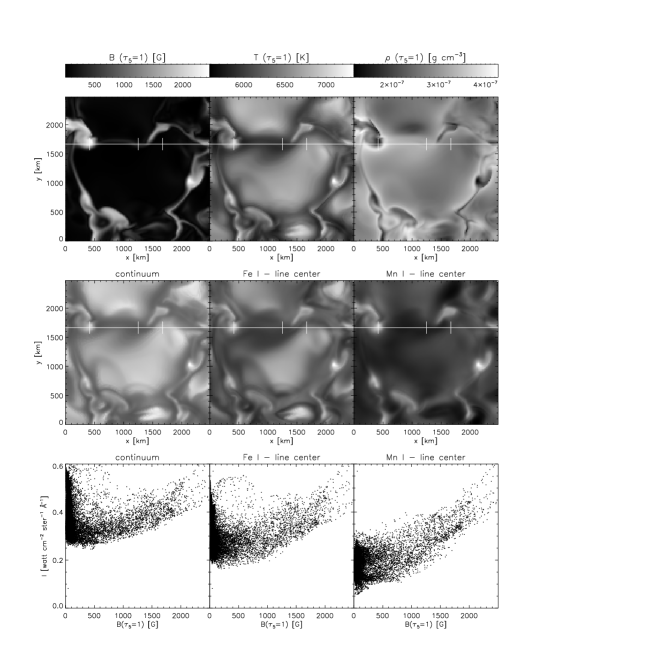
Figure 4: Results from the MURaM snapshot. First row: magnetic field strength, temperature, and gas density across the $\tau_{5}\!=\!1$ continuum-escape surface. Greyscale calibration bars are shown on top. The field is monopolar. The white line specifies the cut used in Figs. 5–8 to display formation parameters in a vertical plane through the simulation volume. It represents a spectrograph slit in Fig. 7. The three superimposed ticks specify locations analyzed in detail in Fig. 7: a magnetic concentration, an intergranular lane, and the edge of the large granule in the center. Second row: synthetic intensity images for the continuum between the two lines and the nominal wavelengths of Fe i 5395.2 Å and Mn i 5394.7 Å. They share the same intensity greyscale. These images represent predicted observations with a telescope matching the MURaM resolution by being diffraction-limited at 2.4-m aperture. The magnetic concentrations (point-like locations with the largest field strength) are about equally bright at all three wavelengths, but the non-magnetic granules (in the center and at the top of the field) are much darker in Mn i 5394.7 Å than in the other two panels. Third row: the same intensities plotted as scatter diagrams per pixel against the magnetic field strength at the $\tau_{5}\!=\!1$ level for that pixel. The upward tails of bright values at large field strength reach the same maxima in all three plots, but the granulation ($B<200$ G) is much darker in Mn i 5394.7 Å than in Fe i 5395.2 Å and the continuum. The first two panels display a pronounced hook shape, but this hook is not present in the Mn i panel. Adding more field therefore gives more spatially-averaged brightening in the Mn i line than in the Fe i line and the continuum. The Mn i line thanks its “unhooking” to its hyperfine structure through which it is less sensitive to the Doppler brightening that affects the Fe i line (and all similar lines) in the granulation.

2.5 Three-dimensional simulation

We use a single snapshot from a time-dependent simulation with the MURaM (MPS/University of Chicago Radiative MHD) code (Vögler & Schüssler (2003); Vögler (2004); Vögler et al. (2005)). MURaM solves the three-dimensional time-dependent MHD equations including non-local and non-grey radiative transfer and accounting for partial ionization.

The particular snapshot used here is taken from a simulation as the one described by Vögler et al. (2005). Its horizontal extent is 6 Mm sampled in 288 grid points per axis, its vertical extent 1.4 Mm with 100 grid points. It was started with a homogeneous vertical seed field of 200 G. Magnetoconvection gave it an appearance similar to active network with strong-field magnetic concentrations in intergranular lanes. A relatively quiet subcube was selected for our line synthesis. It has $2.5\times 2.5$ Mm horizontal extent and contains a large granule and a field-free intergranular lane, in addition to lanes containing magnetic concentrations of varying field strength (Fig. 4).

The line synthesis performed for this paper used the code described above, treating the vertical columns in the subcube as independent lines of sight. The displays below are restricted to the nominal NIST wavelengths of the two lines in Table 1, corresponding to the line centers in a spatially-averaged disk-center intensity atlas as in Fig. 3.

3 Results

3.1 One-dimensional demonstration

Figure 3 presents results of our one-dimensional modeling. The solid curves in the upper panel show the spectral variation of the extinction coefficient for both lines for temperature $T=5000$ K and field strengths $B=0$ G and $B=2000$ G, plus the intermediate profile for $B=1000$ for the Mn i line. For the Fe i line the Zeeman effect produces simple broadening but for the Mn i line the many hyperfine components, each with its own magnetic splitting, cause an intricate pattern shown in the lower part of the inset. The resulting profile widens in the wings but the core first becomes peaked at $B\!=\!1000$ G and then splits into three collective peaks at $B\!=\!2000$ G.

The dotted curves result from inserting temperature $T=7000$ K into the Dopplerwidth but not into other variables, in order to show the effect of larger thermal broadening while keeping all other things equal. The Fe i profile for $B=0$ G looses appreciable amplitude while the Mn i profile does not.

The lower panel of Fig. 3 shows emergent intensity profiles for the two lines. The lowest solid curve is the observed spatially-averaged disk-center spectrum. It is closely matched by the MACKKL modeling when applying standard microturbulence (1 km s^-1) and best-fit macroturbulence (1.28 km s^-1 for Mn i 5394.7 Å, 1.55 km s^-1 for Fe i 5395.2 Å). When this artificial broadening is not applied the computed Fe i line becomes too deep, but the depth of the Mn i line does not change thanks to its flat-bottomed core. The upper curves result from the PLA model with $B=1000$ G, again with (solid) and without (dotted) turbulent smearing. The smearing again affects only the Fe i line. It causes a corresponding shift of the Fe i $\tau_{\lambda}\!=\!1$ location along MACKKL in Fig. 2.

Comparison of these MACKKL and PLA results shows that the spectrum brightens at all wavelengths but most in the Mn i line, by a factor 2. Turbulent smearing does not affect this line but it produces large difference for the Fe i line. In particular, if it is applied to the MACKKL quiet-sun prediction but not to the PLA profile, the Fe i line-center brightness increase is only a factor 1.4.

This difference in line-center brightening suggests that the Fe i line suffers more from thermal broadening and the thermodynamic fine structuring that was traditionally modeled with micro- and macroturbulence. The apparent sensitivity of the Mn i line to magnetic activity may therefore indeed result from non-magnetic quiet-sun Doppler smearing of the Fe i line, lessening the latter’s sensitivity.

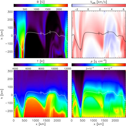
Figure 5: Various quantities in the MURaM snapshot across the vertical plane marked by the white horizontal line in Fig. 4. The upper panels show the magnetic field strength and radial velocity as a function of geometrical height versus horizontal location along the cut. The height scale has $h=0$ km at the mean $\tau_{5}\!=\!1$ level, averaged over all columns. It extends 882 km below and 518 km above that level in the simulation but only the pertinent height range is shown here. The velocity coloring is red for downdraft (redshift) and blue for updraft (blueshift). The lower panels show the temperature and the gas density. The overlaid curves specify $\tau_{5}\!=\!1$ continuum formation depths. The three ticks mark the locations analyzed in Fig. 7.

3.2 Three-dimensional verification

The results from the MURaM simulation are shown in Fig. 4. The three panels in the upper row show basic state parameters across the $\tau_{5}\!=\!1$ surface where $\tau_{5}$ is the continuum optical depth at $\lambda\!=\!5000$ Å determined separately for each simulation column. The middle row displays synthetic intensity images for our three diagnostics: the continuum between the two lines and the nominal line-center wavelengths of Fe i 5395.2 Å and Mn i 5394.7 Å. The bottom row shows these intensities in the form of pixel-by-pixel scatter plots against the magnetic field strength at $\tau_{5}\!=\!1$.

The three images demonstrate directly why Mn i 5394.7 Å shows larger brightness contrast between non-magnetic and magnetic areas: the magnetic bright points reach similar brightness in all three panels but the granulation is markedly darker in this line. Darker granulation implies larger sensitivity to activity, i.e., addition of more magnetic bright points.

The three scatter plots in the bottom row of Fig. 4 quantify this behavior. In the continuum plot at left the darkest pixels lie in field-free or weak-field intergranular lanes. Addition of magnetic field within the lanes brightens them, more for stronger fields, and for the strongest fields almost up to the maximum brightness of field-free granular centers.

Note that in slanted near-limb viewing the magnetic concentrations do not add brightness to dark intergranular lanes but permit deeper viewing into bright granules behind them, adding brightness to the already brightest features and so making faculae brighter than the granular background (see Fig. 1).

The scatter diagram for Fe i 5395.2 Å (bottom-center panel) shows a similar hook shape. The cloud of granulation pixels at left lies lower since the line is an absorption line. However, the pixels with the strongest field still brighten to the same values as in the continuum panel, implying that the line vanishes completely at its nominal wavelength.

The scatter diagram for Mn i 5394.7 Å shows similar behavior, but it loses the hook shape. The line is yet darker in field-free granulation. In this case the corresponding dark cloud of low-field pixels at left does not have an upward tail. However, the upward tail of pixels with increasing field still stretches all the way from the dark lanes to the continuum values, which again implies line vanishing.

If magnetic field is added to field-free granulation, this addition takes away points from the bottom left of the distribution (corresponding to dark intergranular lanes) and adds “magnetic bright points” at the upper right. Its effect is more dramatic in the ensemble average of the Mn i line than in that of the Fe i line because the latter already has bright contributions from field-free granules; in the Fe i line the field-free granulation covers the same brightness range as the field-filled lanes. Thus, field addition means larger spatially-averaged brightness increase in the Mn i line than in the Fe i line.

We conclude that the MURaM synthesis duplicates the sun in having larger brightness response to more activity in the Mn i line than in the Fe i line – not via chromospheric emission but through showing granulation darker.

3.3 Explanation

Unlike the sun, the MURaM simulation offers the opportunity to not only inspect the emergent spectrum but also to dissect the behavior of pertinent physical parameters throughout the simulation volume. So instead of ending this paper here with the above conclusion that neither a chromosphere nor NLTE coupling to Mg ii h & k are needed to reproduce the activity sensitivity of Mn i 5394.7 Å, we add analysis of the MURaM results to diagnose why the granulation appears darker in the Mn i line – or rather, why it appears brighter in the Fe i line – and so earn our use of the term “explanation” in the title of this paper.

The white line with three ticks in the grey-scale panels of Fig. 4 specifies the spatial samples that are selected in Figs. 5–8. This particular cut and the tick locations were chosen to sample a strong-field magnetic concentration that appears as a bright point in the intensity images (lefthand tick), a non-magnetic dark lane (middle tick), and a granule (righthand tick). Unfortunately, this cut samples only the edge rather than the center of the large granule covering the center part of the field but otherwise we wouldn’t have sampled both a bright point and a non-magnetic lane. A magnetic lane less extreme than the bright point is sampled at the far right.

Figure 5 diagnoses MURaM physics in the vertical plane defined by this cut. It shows behavior that is characteristic of solar magnetoconvection near the surface. The overlaid curves specify the $\tau_{5}\!=\!1$ continuum surface. The very low gas density (4th panel) in the magnetic concentration at $x\approx 400$ km produces a large Wilson depression of about 200 km. The deep dip in the $\tau_{5}\!=\!1$ curve so samples relatively high temperature, as well as a relatively flat vertical temperature gradient. The intergranular lane at $x\approx 1300$ km combines low temperature with high density and strong downdraft; the granule edge at $x\approx 1650$ km combines higher temperature with gentler updraft and low subsurface density.

Figure 6 repeats this vertical-plane display of temperature and density but plotted per column on the radial optical depth scale that belongs to each diagnostic. The panels in the first and second columns show the atmosphere “as seen” by each spectral feature at its nominal wavelength. The dotted horizontal lines at $\log\tau_{\lambda}\!=\!0$ indicate their formation heights. The solid curves are the $\tau_{5}\!=\!1$ locations. The third column shows relative behavior of the corresponding opacities in the form of fractional lower-level population variations.

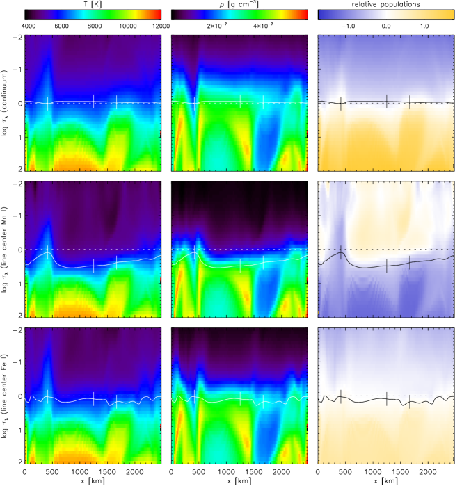
Figure 6: Temperature, gas density, and population variations across the vertical cut through the MURaM simulation plotted per column on radial optical depth scales for the nominal continuum (top row), Mn i 5394.7 Å (middle row), and Fe i 5395.2 Å (bottom row) wavelengths. The solid curves specify $\tau_{5}\!=\!1$ depths, the horizontal dotted lines feature-specific $\tau_{\lambda}\!=\!1$ depths. The third column displays fractional population offsets. These are the lower-level populations for H${}^{{}^{{}_{-}}}\!$ bound-free transitions, the Mn i line, and the Fe i line, each normalized by the total element density (hydrogen, manganese, iron) per location and shown in logarithmic units scaled to the mean value at $\tau_{\lambda}\!=\!1$ along the cut. Positive offsets are colored amber, negative bluish. The scale runs from $-1.8$ to $+1.8$.

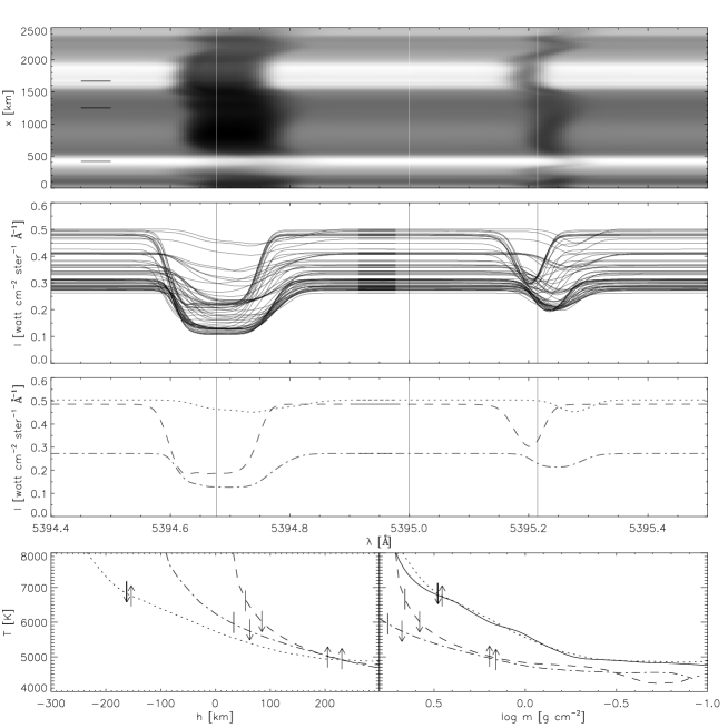
Figure 7: Further analysis of the formation of Mn i 5394.7 Å, Fe i 5395.2 Å, and the intermediate continuum in the MURaM simulation. Top panel: spectrum synthesized from the computed emergent intensities. The vertical coordinate corresponds to the $x$ sampling along the cut specified in Fig. 4. The three black horizontal markers correspond to the ticks selecting the bright point (lowest), field-free intergranular lane (middle), and granule edge (highest). The three vertical lines specify the nominal wavelengths for Mn i 5394.7 Å (left), Fe i 5395.2 Å (right), and the intermediate continuum (center). Second panel: spectral profiles for every second pixel along the cut. Third panel: spectral profiles for the three locations specified by ticks in Fig. 4 and black markers in the top panel. Dotted: magnetic concentration. Dot-dashed: intergranular lane. Dashed: granule edge. Bottom panels: temperature stratifications for the three selected locations, at left against geometrical height, at right against column mass as in Fig. 2. The solid curve is the PLA model, as in Fig. 2. The tick marks specify the $\tau_{\lambda}\!=\!1$ locations for the nominal wavelengths of Mn i 5394.7 Å (upward arrows), of Fe i 5395.2 Å (downward arrows), and of the continuum in between (arrowless). In the magnetic concentration the Fe i 5395.2 Å tick coincides nearly with the continuum one. The Wilson depression is much larger for the Mn i line than for the continuum and the Fe i line.

The top panels of Fig. 6 show only slight differences between the $\tau\!=\!1$ locations along the cut. The magnetic concentration has an appreciable hump in $T(\tau_{\lambda})$ and dip in $\rho(\tau_{\lambda})$ around $\tau_{5}\!=\!1$. The relatively high temperature and low density there combine into increased electron-donor ionization. This is illustrated by the sixth panel showing the fractional population variation of the lower level of Mn i 5394.7 Å, which is the Mn i ground state. Its behavior equals the depletion by manganese ionization apart from a minor correction for the temperature sensitivity of the Mn i partition function. Manganese has too small abundance to be an important electron donor, but it ionizes similarly to iron (Table 1) so that this panel illustrates characteristic electron-donor ionization, with neutral-stage depletion occurring within magnetic concentrations and at large depth. The corresponding increase of the free-electron density produces larger H${}^{{}^{{}_{-}}}\!$ opacity, evident as overall color gradient reversal between the top and center panels in the third column. It results in an upward enhancement peak at the magnetic concentration in the H${}^{{}^{{}_{-}}}\!$ population panel. This relative increase of the continuum opacity explains that $\tau_{\lambda}\!=\!1$ is reached at lower density in the magnetic concentration than in the adjacent intergranular lane (second panel); the Wilson depression is smaller than one would estimate from pressure balancing alone. The flat temperature gradient in the magnetic concentration produces a marked upward extension in $T(\tau_{\lambda})$ in the first panel. It contributes brightness enhancement along much of the intensity contribution function and so makes magnetic concentrations appear bright with respect to non-magnetic lanes. However, the hook pattern in the continuum scatter plot in Fig. 4 shows that this lane brightening does not exceed granular brightness.

The center row of Fig. 6 shows that Mn i 5394.7 Å is generally formed higher than the continuum, but not in the magnetic concentration where the upward hump in the $\tau_{5}\!=\!1$ curve nearly reaches the $\tau_{\lambda}\!=\!1$ level. This is because the relatively high temperature and low density there increase the degree of manganese ionization, as evident in the third panel which shows a marked upward blue extension. The line weakens so much that the brightest Mn i pixels in Fig. 4 reach the same intensity as in the continuum, also sampling the upward high-temperature extension (first column). Conversely, the largest line-to-continuous opacity ratio (i.e., the largest separation between the $\tau_{\lambda}\!=\!1$ and $\tau_{5}\!=\!1$ locations) is reached along the intergranular lane where the neutral-stage population is larger due to relatively large density and low temperature. Thus, the curve separation maps the variation of the fractional ionization along the dotted line. Since the temperature increases inward anywhere, the deeper sampling within the magnetic concentration and the higher sampling in the granulation, especially in the lanes, together increase the brightness contrast between bright point and granulation compared to that in the continuum. This effect of increased ionization is similar to the effect of CH dissociation in the G band and reduced damping in the H $\alpha$ wings within magnetic concentrations. It enhances the magnetic lane brightening so that that exceeds granular brightnesses, undoing the hook shape of the continuum scatter plot.

The bottom row of Fig. 6 shows the corresponding plots for Fe i 5395.2 Å. Iron and manganese ionize similarly so that low-excitation Fe i lines suffer the same depletion in magnetic concentrations. However, Fe i 5395.2 Å is a high-excitation line; its Boltzmann sensitivity to higher temperature largely compensates for the enhanced ionization so that the panel in the third column looks much more like the top one for H${}^{{}^{{}_{-}}}\!$ than like the second one for Mn i 5394.7 Å: the overall color gradient flips back again. The line again vanishes in the magnetic concentration, so that the strongest-field pixels in Fig. 4 again reach the continuum intensities. One might expect that the curve separation in the bottom panels would follow the temperature pattern under the dotted line in the first column, but this is not the case; for example, the line also nearly vanishes (at its nominal wavelength) in the intergranular lane. This discordant variation is caused by the Dopplershifts imposed on the line extinction by the flows displayed in the upper-right panel of Fig. 5. Comparison shows that the unsigned amplitude of the flow variation along the cut at $100-200$ km above the $\tau_{5}\!=\!1$ curve there is mapped precisely into reversed modulation of the $\tau_{5}\!=\!1$ curve for Fe i 5395.2 Å here. Thus, the line vanishes because it is shifted aside from its nominal wavelength.

We demonstrate the Doppler-related formation differences between the two lines further in Fig. 7. The upper two panels display spectral representations along the cut defined in Fig. 4, in the form of a spectral image and of profile samples. The top panel shows what would have appeared in an observational spectrogram from a telescope with MURaM resolution. Both lines show a bright “line gap” in the magnetic concentration near the bottom. At $x\approx 2500$ km the intergranular lane with less strong field still causes a noticeable gap. Large Dopplershifts occur in the field-free lane and the granular edge.

The second panel shows the product of data reduction of this spectrogram. Both panels illustrate that the line-center intensity of the Mn i line is not very sensitive to Dopplershifts, whereas the Fe i line shifts well away from its nominal wavelength nearly everywhere. It also weakens more in the granule edge from larger thermal broadening (Fig. 3). Taking the spatial mean at each nominal wavelength does a fair job of intensity averaging for the Mn i line but misses nearly all dark cores in the Fe i line, especially in the lanes but also in granules. Note that this particular cut does not represent hot granules well; more samples of these would add many profiles with weakened cores blueward of the nominal Fe i wavelength.

The third panel shows the spectral profiles for the three sample locations along the cut. The nominal Fe i line-center wavelength misses all three cores! Thus, the brightness average at this wavelength is much higher than it would be for an undisturbed line of this opacity. The Mn i line-center wavelength, however, only misses the deepest part of the magnetic-concentration profile which is weak anyhow. This disparity in Doppler sensitivity explains why the granulation in Fig. 4 is much darker in Mn i 5394.7 Å than in Fe i 5395.2 Å.

Also note the sharpening of the Mn i line profile from boxy to more pointed in some of the intermediate profiles in the second panel, which follows the extinction coefficient behavior in Fig. 3. It contributes to the decrease in equivalent width of Mn i 5394.7 Å at larger activity, which is not analyzed here.

The bottom panels of Fig. 7 show the vertical temperature stratifications at the three sample locations, at left against geometrical height with $h\!=\!0$ at $\tau_{5}\!=\!1$ for the simulation mean, at right against column mass per feature. These graphs link the simulation results back to the classical fluxtube modeling in Sect. 3.1. They display familiar properties of granulation and magnetic concentrations: the temperature gradient is steepest in granules, flatter in intergranular lanes, with a mid-photosphere cross-over producing “reversed granulation”, and flattest in fluxtubes. The heights of formation, marked by ticks specifying the $\tau_{\lambda}\!=\!1$ locations, are similar per line in the granular edge and the lane but much deeper in the magnetic concentration which is the coolest feature at equal geometrical height but the hottest at equal column mass and at the $\tau_{\rm cont}\!=\!1$ location per feature. The Wilson depression is about 200 km in the continuum and twice as large for the Mn i line through enhanced ionization within the magnetic concentration, but not for the Fe i line due to its Doppler-deepened granulation sampling. Both lines weaken severely in the magnetic concentration through this deep sampling, and both are redshifted away from their nominal wavelength, Fe i 5395.2 Å all the way so that its $\tau_{\lambda}\!=\!1$ tick coincides with the continuum one.

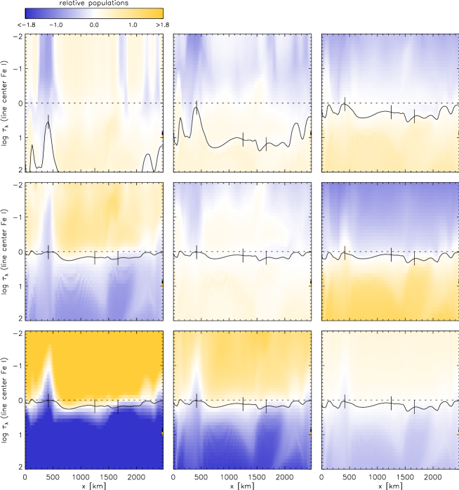
Figure 8: The effect of excitation energy and line strength on Fe i line formation. Each panel is the fractional population of the lower level of an artificial line comparable to Fe i 5395.2 Å along the cut through the MURaM simulation defined in Fig. 4, again shown on nominal line-center optical depth scales, normalized to the mean value along the dotted line, and with the same logarithmic color coding as in the third column of Fig. 6, clipped at offsets $-1.8$ and $+1.8$. The solid curves are again the $\tau_{5}\!=\!1$ locations for the continuum at 5000 Å, the dashed lines the line-center $\tau_{\lambda}\!=\!1$ formation indication. Top row: the Fe i 5395.2 Å line at excitation energy 2, 3, and 4 eV, respectively. The corresponding mean Boltzmann factors at $\tau_{\lambda}\!=\!1$ are $1.2\times 10^{-3}$, $1.7\times 10^{-4}$, and $5.2\times 10^{-5}$. Second row: the Fe i 5395.2 Å at excitation energy 0, 3, and 6 eV but with the oscillator strength scaled to maintain the same line strength in the emergent spectrum that Fe i 5395.2 Å shows (by $25\times 10^{-3}$, 25 and $25\times 10^{3}$, respectively). Bottom row: idem, but the color coding now measures deviations from the Milne-Eddington approximation by showing the lower-level population divided by the H${}^{{}^{{}_{-}}}\!$ population. The leftmost panel is severely clipped. The Milne-Eddington approximation improves dramatically with higher excitaton.

4 Discussion

4.1 Comparison of 1D modeling and 3D simulation

We have used both classical empirical fluxtube modeling (Sect. 3.1) and modern MHD simulation (Sect. 3.2). The bottom panels of Fig. 7 connect the latter with the former. The righthand panel shows remarkably close agreement between the PLA model and the MURaM magnetic-concentration stratification. This may be taken as mutual vindication of these very different techniques, but not as proof of correctness since both assumed LTE ionization (discussed below) while the sun does not.

The simulation resolves the granular Dopplershifts that were emulated by turbulence in the classical modeling. The simulation analysis in Sect. 3.3 confirms that Mn i 5394.7 Å activity-brightens more than Fe i 5395.2 Å  because its intrinsic hyperfine-structure broadening suppresses thermal and Doppler brightening in non-magnetic granulation. This was already indicated by the 1D demonstration in Fig. 3.

4.2 Validity of LTE

We have assumed LTE throughout this paper. In Sect. 2.3 we noted that the most likely departure from LTE which may affect our two lines is loss of opacity through radiative overionization, in locations with steep temperature gradients where the angle-averaged intensity exceeds the Planck function in ultraviolet photo-ionization edges (see e.g., Rutten (2003) for more explanation). The steepest temperature gradients in Fig. 5 occur not along radial columns but transverse through the magnetic concentration. Therefore, the ionization which contributes to the vanishing of the Mn i line from the corresponding bright point may be underestimated. If so, the H${}^{{}^{{}_{-}}}\!$ opacity is equally underestimated. However, the MURaM simulation itself assumes LTE with coarse spectral sampling and is likely to differ intrinsically if NLTE overionization affecting the H${}^{{}^{{}_{-}}}\!$ opacity is taken into account. Such overionization was similarly neglected in the empirical construction of the PLA model based on Fe i-line spectropolarimetry assuming LTE to define the optical depth scales. Improvement requires non-trivial evaluation of the ultraviolet line haze.

4.3 Extension to other lines

We have demonstrated and analyzed Doppler brightening in detail only for Mn i 5394.7 Å and Fe i 5395.2 Å. The first may be taken to exemplify all lines with wide boxy extinction profiles, the second all lines with narrow peaked profiles, i.e., almost all other photospheric lines. Figure 8 serves to demonstrate the latter generalization by extending the MURaM synthesis to a range of artificial Fe i lines by simply placing Fe i 5395.2 Å at other excitation energies. The first two rows again display relative population variations across the simulation cut using the same color coding as in the third column of Fig. 6. The top row of Fig. 8 combines the effects of the Boltzmann factor on the amplitude of the line extinction and on its temperature sensitivity. The second row isolates the latter by making each line just as weak as Fe i 5395.2 Å.

The first panel of Fig. 8 is included only for illustration because this artificial line is already too strong for reliable synthesis from our simulation and would also suffer appreciable departures from LTE if it existed in reality (see Rutten & Kostik (1982)). It is formed near the top of the simulation volume which sets the columnar structure in the upper part; the sizable vertical flows there impose the separation between the two $\tau\!=\!1$ curves. In reality, very strong Fe i lines suffer less convective and thermal Doppler weakening in their cores which explains the observation by Malanushenko et al. (2004) that the strongest Fe i lines show some (but only slight) global activity modulation. Even that modulation has nothing to do with the chromosphere! The second and third panel describe deeper line formation with steeper gradients. Their $\tau\!=\!1$ separations also demonstrate Doppler modulation. Thus, Doppler weakening affects these three lines just as it affects Fe i 5395.2 Å.

The second row of Fig. 8 illustrates the effect of Boltzmann temperature sensitivity at given emergent line strength. The first panel describes the Fe i ground state and is nearly the same as the sixth panel of Fig. 6. Towards higher excitation energy the Boltzmann increase compensates more of the depletion by ionization. In the center panel the population offset gradients are very flat; at right, they are reversed so that the population variation mimics the behavior of H${}^{{}^{{}_{-}}}\!$ in the third panel of Fig. 6 closely, although at slightly smaller amplitude. The Doppler modulation of the $\tau\!=\!1$ separation remains similar, irrespective of this gradient reversal in fractional population distribution. Thus, Doppler brightening affects all photospheric Fe i lines similarly.

The third row of Fig. 8 repeats this test in terms of the Milne-Eddington approximation (constant line-to-continuum opacity ratio with height) which is often assumed in photospheric polarimetry (e.g., Auer et al. (1977); Skumanich & Lites (1987); Westendorp Plaza et al. (1998); Orozco Suárez et al. (2007)). At left the combination of Fe i depletion by ionization and the corresponding increase in H${}^{{}^{{}_{-}}}\!$ opacity implies squaring of the population offsets or twice steeper gradients in this logarithmic plot than in the second row. The Milne-Eddington approximation fails badly but least within the magnetic concentration. It improves with excitation energy through the Boltzmann compensation. The panel at right shows the residue from subtracting the sixth panel in this figure from the third panel in Fig. 6, resulting in rather small deviations. This behavior was shown earlier in Fig. 3 of Rutten & van der Zalm (1984; reprinted in Fig. 9.2 of Rutten (2003)).

4.4 Irradiance modeling

In this paper we have not made the step from radial viewing to full-disk averaging. The demonstration in Sect. 3.1 used Solanki’s one-dimensional empirical model for a fluxtube in plage but without adding flaring fluxtube geometry, granular presence next to a fluxtube and behind it in slanted facular viewing, multiple-tube interface geometry, spatial averaging over these geometries, the multi-angle evaluation needed to emulate center-to-limb viewing, and without full-disk averaging and consideration of spatial distributions over the solar surface and their variations with the solar cycle. All these non-trivial aspects would need careful quantification to expand the demonstration of enhanced sensitivity in Sect. 3.1 into a quantitative estimate for comparison with Livingston’s irradiance data. The simulations in Sect. 3.2 yielded profile synthesis for a small area of solar surface containing strong-field concentrations that may be considered more realistic than idealized magnetostatic fluxtubes but, nevertheless, generation of full-disk signals comparable to Livingston’s data still requires all the above quantifications. This effort is not done here.

In contrast, the step from one-dimensional line synthesis to emulation of the full-disk and cycle-dependent integrated signal was recently made by Danilović et al. (2007) using the SATIRE (Spectral And Total Irradiance Reconstruction) approach of Fligge et al. (2000), Krivova et al. (2003) and Wenzler et al. (2005, 2006). In this technique the spatial distributions of spots and plage are extracted from full-disk magnetograms and continuum images to derive disk-coverage distributions throughout the more recent activity cycles. Each component (quiet sun, plage, spots) is represented by a standard one-dimensional model atmosphere. The first two are shown as dotted curves in Fig. 2. The lower one for quiet sun is the radiative equilibrium model of Kurucz (1979, 1992a, 1992b) which is nearly identical to MACKKL. The upper one for plage was made by Unruh et al. (1999) by smoothing model P of Fontenla et al. (1993) and deleting its chromospheric temperature rise. For spots a Kurucz radiative-equilibrium model with low effective temperature is used, not shown here. Danilović et al. (2007) found that using these models with the empirically established SATIRE coverage fractions gives a good reproduction of Livingston’s data both for Mn i 5394.7 Å and Fe i 5395.2 Å.

Such use of the dotted models in Fig. 2 is an ad-hoc trick to reproduce the larger brightness of plage. The Mn i 5394.7 Å line activity-brightens more than Fe i 5395.2 Å in this simplistic modeling because it is a stronger line, hence formed higher, hence getting more out of the divergence between the two models with height. Any line as strong would show the same brightening. Stronger lines would brighten more; in particular, Fe i lines with deeper cores than Mn i 5394.7 Å would show larger activity modulation in conflict with the observations.

Actually, as illustrated in Fig. 1 and demonstrated in Figs. 4–8, plage thanks its disk-center brightening in any photospheric diagnostic not to being hotter at equal height but to below-the-surface viewing of hot-wall heat within magnetic concentrations. The SATIRE modeling does not evaluate Wilson depressions, but as long as the SATIRE models are used in one-dimensional radial fashion on their own column mass or optical depth scale this does not matter. In this sense the Unruh plage model does recognize that the local temperature gradient around local $\tau\!=\!1$ within magnetic concentrations tends to be less steep than in the granulation, as in the bottom panels of Fig. 7. However, the approximation breaks down for non-vertical fluxtube viewing for which the “Zürich wine-glass” geometry of Bünte et al. (1993) with slanted rays passing through the glasses was a much more realistic description, and it fails for limbward faculae because slanted viewing of hot granule innards through empty fluxtubes (Fig. 1) should not be described by the vertical temperature stratification within magnetic concentrations.

Plage and faculae were much better treated by the older Solanki-style fluxtube models which diverge with depth instead of with height between magnetic and non-magnetic (compare the PLA and Unruh plage models in Fig. 2 and PLA with the MURaM stratification in Fig. 7). Obviously, outward divergence supplies a zero-order approximation to increasing facular contrast in limbward viewing, but no more than that and inherently wrong.

The same criticisms apply to the similar photospheric feature modeling through outward-diverging temperature stratifications by e.g., Fontenla et al. (1993, 2006), who add more ad-hoc adjustment parameters in the form of a deep-seated chromospheric temperature rise, comparable to the ones invoked by Doyle et al. (2001), that was rightfully removed by Unruh et al. (1999) in their plage model – the chromosphere has nothing to do with network and plage visibility in photospheric diagnostics.

Nevertheless, the success of the SATIRE modeling by Danilović et al. (2007) implies that, given any trick to make a single magnetic concentration brighter in Mn i 5394.7 Å than in Fe i 5395.2 Å by the amount given by SATIRE’s two-model divergence, that trick will reproduce Livingston’s data similarly. Thus, although we have not performed any full-disk modeling, our trick is likely to reproduce these data too. Our trick entails better understanding of why Mn i lines activity-brighten more than other lines: the latter brighten more in normal granulation.

5 Conclusion

The explanation of the activity sensitivity of Mn i 5394.7 Å concerns deep-photosphere line formation only. Intergranular magnetic concentrations brighten with respect to field-free intergranular lanes in any photospheric diagnostic through deep radiation escape sampling relatively high and flat-gradient temperatures (Figs. 5 and 6). For normal, narrow photospheric lines this brightening has less effect in full-disk averaging through their loss of line depth in normal granulation (Fig. 7) that was traditionally mimicked by applying micro- and macroturbulent smearing (Fig. 3). The flat-bottomed profile which Mn i 5394.7 Å possesses thanks to its hyperfine structure (Fig. 3) makes this line much less susceptible to granular Doppler smearing and thermal broadening so that it weakens less in normal granulation (Fig. 7) and so displays larger mean brightness contrast between quiet and magnetic areas (Fig. 4).

The Mn i 5394.7 Å line is therefore an unsigned proxy magnetometer sensitive to the magnetic concentrations that constitute on-disk network and plage and near-limb faculae, through Wilson-depression viewing of subsurface bright-wall heat near disk center and through slanted facular viewing into hot granules near the limb (Fig. 1). In solar irradiance monitoring Mn i 5394.7 Å tracks well with the Ca ii  H & K and Mg ii  h & k core brightnesses because these also respond to magnetic concentrations, although through unidentified magnetic chromosphere heating that does not affect the Mn i lines, neither directly nor through interlocking to Mg ii h & k.

As a proxy magnetometer Mn i 5394.7 Å is similar to the G band in which the contrast enhancement arises from the general addition of CH line opacity and local reduction of that through dissociation in magnetic concentrations, and to the extended blue wings of strong lines in which the contrast enhancement arises from the general addition of line opacity with reduction of that through lesser damping in magnetic concentrations plus Doppler flattening of the granular contrast (Leenaarts et al. (2006b)). These are all sufficiently wide in wavelength to not suffer from the granular Doppler smearing that spoils the contrast for the centers of narrow lines. The G band is the most useful of these proxies by being a wide-band spectral feature in the blue. Qua contrast, the blue wing of H $\alpha$ is probably the best of all (Leenaarts et al. (2006a)), but not for full-disk irradiance monitoring since its photospheric magnetic-concentration brightening is sometimes obscured by overlying dark blue-shifted and/or heat-widened chromospheric fibril absorption.

We conclude that the principal usefulness of photospheric Mn i lines lies not in their unusual activity sensitivity but in their hyperfine-structured richness as weak-field diagnostic in full-Stokes polarimetry with high angular resolution and sensitivity (e.g., Sánchez Almeida et al. (2008)).