The distribution of ejected subhalos and its implication for halo assembly bias

Abstract

Using a high-resolution cosmological $N$-body simulation, we identify the ejected population of subhalos, which are halos at redshift $z=0$ but were once contained in more massive ‘host’ halos at high redshifts. The fraction of the ejected subhalos in the total halo population of the same mass ranges from 9% to 4% for halo masses from $\sim 10^{11}$ to $\sim 10^{12}\,h^{-1}{\rm M_{\odot}}$. Most of the ejected subhalos are distributed within 4 times the virial radius of their hosts. These ejected subhalos have distinct velocity distribution around their hosts in comparison to normal halos. The number of subhalos ejected from a host of given mass increases with the assembly redshift of the host. Ejected subhalos in general reside in high-density regions, and have a much higher bias parameter than normal halos of the same mass. They also have earlier assembly times, so that they contribute to the assembly bias of dark matter halos seen in cosmological simulations. However, the assembly bias is not dominated by the ejected population, indicating that large-scale environmental effects on normal halos are the main source for the assembly bias.

1 Introduction

In the standard cold dark matter (CDM) paradigm of structure formation, galaxies are supposed to form and evolve in dark matter halos. The study of the clustering properties of dark matter halos and their relation to galaxy clustering can thus help us to understand the connection between halos and galaxies, and hence to understand how galaxies form and evolve in dark matter halos. It is now well known that the correlation strength of dark matter halos depends strongly on halo mass (e.g., Mo & White 1996; Mo et al. 1997; Jing 1998; Sheth & Tormen 1998; Sheth, Mo & Tormen 2001; Seljak & Warren 2004), and this dependence, which is referred to as the halo bias, has been widely used to understand the clustering of galaxies via the halo occupation model (e.g., Jing, Mo & Börner 1998; Peacock & Smith 2000), and the conditional luminosity function model (e.g., Yang, Mo & van den Bosch 2003).

More recently, a number of independent investigations have shown that the halo bias depends not only on the mass but also assembly time of dark matter halos, in the sense that halos of a given mass, particularly low-mass ones, are more strongly correlated if they assembled half of their masses earlier (e.g. Gao et al. 2005; Harker et al. 2006; Zhu et al. 2006; Wechsler et al. 2006; Jing, Suto & Mo 2007; Wetzel et al. 2007; Bett et al. 2007; Gao et al. 2007; Li et al. 2008). The origin of this assembly-time dependence of the halo bias, referred to in the literature as the halo assembly bias, is important to understand, because if it is due to a process that can also affect galaxy formation and evolution in a halo then it would affect our interpretation of galaxy clustering in terms of halo clustering. There have been theoretical investigations about the origin of the halo assembly bias (e.g. Wang et al. 2007; Sandvik et al. 2007; Desjacques 2007; Keselman & Nusser 2007; Dalal et al. 2008; Hahn et al. 2008). Wang et al. (2007) find that old, small halos tend to live near massive halos, and suggest that the tidal truncation of accretion may be responsible for the assembly bias. This is consistent with the result of Maulbetsch et al. (2007), who find that most of the small halos in high-density regions have ceased accretion. Along this line, Desjacques (2007) develops an ellipsoidal collapse model which takes into account the large-scale tidal field, while Keselman & Nusser (2007) perform simulations using the Zel’dovich (PZ) approximation to take into account the large-scale tidal effects. Both investigations find significant dependence of halo bias on halo assembly history, indicating that large-scale tidal effects may play an important role in producing the assembly bias. More recently, Ludlow et al. (2008, hereafter L08) study in detail 5 simulations of dark matter halos and find that a significant fraction of small halos are physically associated with nearby massive halos. These small halos have been once inside their host halos but were ejected due to interactions with other subhalos (see also Lin et al. 2003; Wang et al. 2005; Gill, Knebe, & Gibson 2005). L08 suggest that these ejected subhalos may be responsible for the enhanced clustering of old small halos. However, because of the small volume of their simulations, they were not able to quantify whether the ejected population alone can account for the assembly bias seen in cosmological simulations.

In this paper we use a high-resolution $N$-body simulation in a cosmological box to study the distribution of ejected subhalos in space and to quantify the contribution of this population of halos to the assembly bias. The outline of the paper is as follows. In Section 2 we describe briefly the simulation used and how ejected subhalos are identified. In Section 3 we study the distribution of the ejected subhalos in phase space, and how the distribution depends on the properties of their hosts. In Section 4 we examine the contribution of the ejected subhalos to the assembly bias obtained in our simulation. Finally, in Section 5, we discuss and summarize our results.

2 Simulation and Dark Matter halos

2.1 Numerical simulation and halo identification

The simulation used in this paper is obtained with the ${\rm P^{3}M}$ code described in Jing & Suto (2002). It assumes a spatially-flat $\Lambda$CDM model, with density parameters $\Omega_{\rm m}=0.3$ and $\Omega_{\Lambda}=0.7$. The CDM power spectrum is assumed to be that given by Bardeen et al. (1986) with a shape parameter $\Gamma=\Omega_{\rm m}h=0.2$ and an amplitude specified by $\sigma_{8}=0.9$. The CDM density field is traced with $512^{3}$ particles, each having a mass $M_{p}\sim 6.2\times 10^{8}$$\,h^{-1}{\rm M_{\odot}}$, in a cubic box of 100 $\,h^{-1}{\rm{Mpc}}$. The softening length is $\sim 10\,h^{-1}{\rm{kpc}}$ (S2 type). The simulation, started at redshift 72, is evolved with 5000 time steps to the present day ($z=0$) and has 60 outputs from $z=15$, equally spaced in $\log(1+z)$. Dark matter halos were identified with a friends-of-friends algorithm with a link length that is $0.2$ times the mean particle separation.

2.2 Ejected subhalos

Our analysis focuses on the ejected subhalos which are identified as FOF halos at redshift $z=0$. In order to determine whether a halo is an ejected subhalo or a normal halo, a detailed merging tree for each FOF halo is required so that we can trace a FOF halo back in time to see whether it has ever been within another FOF halo. We consider a halo at any given redshift $z>0$ to be a progenitor of a descendant halo in the next output, if more than half of its particles are found in the descendant. A given halo in general can have one or more progenitors but only one descendant. We can therefore use the uniqueness of the descendant to build up the merging tree for each halo. Each FOF halo at the present time has one and only one merging tree to describe its assembly history. There is a small fraction of halos at $z>0$ that have dispersed and have no descendant at $z=0$. These halos are excluded in our analysis. The merging tree of a halo can be used to verify whether an isolated FOF halo (called halo ‘A’) at $z=0$ was accreted into a massive halo earlier. To do this, we search in the next snapshot (in reverse order of time) a ‘host’ halo that contains at least half of the particles in halo ‘A’, but does not belong to the merging tree of halo ‘A’. If no such a ‘host’ halo is found in this snapshot, we take the most massive progenitor of halo ‘A’ in this snapshot and repeat the same procedure for this progenitor as we have carried out for halo ‘A’. This procedure is continued until a ‘host’ halo is found or the tree ends. If such a ‘host’ halo is found, halo ‘A’ is then identified as an ejected subhalo, which is said to be ejected at the time, $t_{\rm e}$, when the ‘host’ halo is found. Note that the ejection time, $t_{\rm e}$, is defined to be the time of the snapshot at which the ‘host’ and ‘ejected’ halos were just separated from the same FOF group. We also define an accretion time, $t_{\rm a}$, as the time when half of the particles in the most massive progenitor of halo ‘A’ at ejection time is first contained in the most massive progenitor of its ‘host’. If no ‘host’ halo is found before the merging tree ends, halo ‘A’ is said to be a normal halo. Applying this method to all halos at $z=0$, we construct a catalogue of ejected subhalos, and the total number of ejected subhalos is listed in Table 1 in three mass ranges. We denote the masses of an ejected subhalo and of the corresponding ‘host’ halo at any time $t$ as $M_{\rm s}(t)$ and $M_{\rm host}(t)$, respectively, and we use $M_{\rm h}$ to denote the mass of a normal halo at redshift $z=0$. Thus, $M_{\rm host}(t_{\rm e})$ is the mass of the ‘host’ halo at the time of ejection, and $M_{\rm host}(t_{0})$ is the mass of the descendant of the ‘host’ at the present time, $t_{0}$.

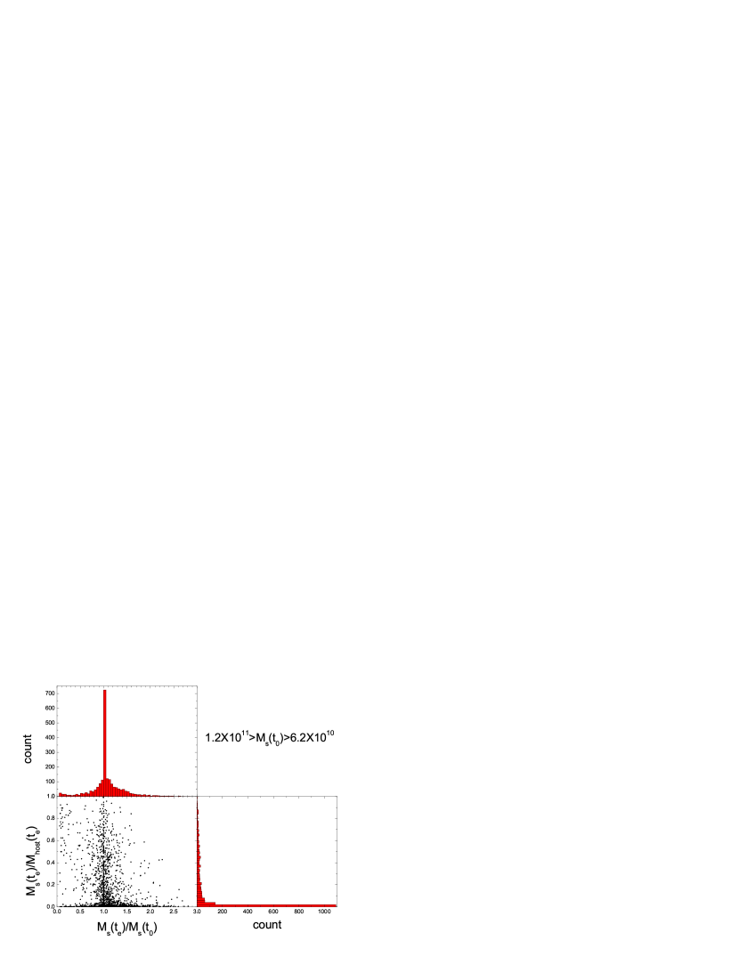
Figure 1: The lower-right panel shows $M_{\rm s}(t_{\rm e})/M_{\rm host}(t_{\rm e})$ as a function of $M_{\rm s}(t_{\rm e})/M_{\rm s}(t_{0})$ for ejected subhalos with masses between $6.2\times 10^{10}$ and $1.2\times 10^{11}\,h^{-1}{\rm M_{\odot}}$. The upper and lower-right panels are the histograms for $M_{\rm s}(t_{\rm e})/M_{\rm s}(t_{0})$ and $M_{\rm s}(t_{\rm e})/M_{\rm host}(t_{\rm e})$, respectively.

In Fig. 1 we show $M_{\rm s}(t_{\rm e})/M_{\rm host}(t_{\rm e})$ versus $M_{\rm s}(t_{\rm e})/M_{\rm s}(t_{0})$ for halos with $6.2\times 10^{10}<M_{\rm s}(t_{0})<1.2\times 10^{11}\,h^{-1}{\rm M_{\odot}}$. The corresponding histograms for $M_{\rm s}(t_{\rm e})/M_{\rm s}(t_{0})$ and $M_{\rm s}(t_{\rm e})/M_{\rm host}(t_{\rm e})$ are also shown in the figure. The results for other mass ranges are similar and are not shown. As one can see, the majority of the ejected subhalos were ejected by ‘host’ halos that are much more massive than the ejected subhalos themselves. Only small fraction of halos are ejected by host halos with comparable masses: about 11% (34%) of ejected subhalos have a mass larger than 0.5 (0.1) times of their host halo mass. Furthermore, most of the ejected halos have masses that are similar to those at the time of ejection, indicating that mass loss or accretion after ejection is not severe. However, the distribution has two extended tails, and the 10th and 90th percentile values are 0.73 and 1.48, respectively. In our analysis, we remove all systems with $M_{\rm s}(t_{\rm e})/M_{\rm s}(t_{0})<0.5$, i.e. the halos that have accreted more than their initial masses after ejection. Note that the removed halos is a very small fraction, about 5%, of the total sample (Table 1). Including them does not have any significant impact on the results to be presented below. After the removal, the final numbers of the ejected subhalos in different halo mass ranges are also given in Table 1. For comparison, we also list the corresponding numbers for all (ejected plus normal) halos in these mass ranges. About 9% - 4% of all the halos in the mass ranges considered are ejected subhalos, and the fraction decreases with increasing $M_{\rm s}(t_{0})$.

Table 1: The number of ejected subhalos in various samples

$M_{\rm s}/(\,h^{-1}{\rm M_{\odot}})$	$[6.2\times 10^{10},1.2\times 10^{11}]$	$[1.2\times 10^{11},3.7\times 10^{11}]$	$[3.7\times 10^{11},10^{12}]$
Ejected (total)	2115	1076	231
Ejected (final)	2009	1036	220
Ejected$+$Normal	22697	16490	5850

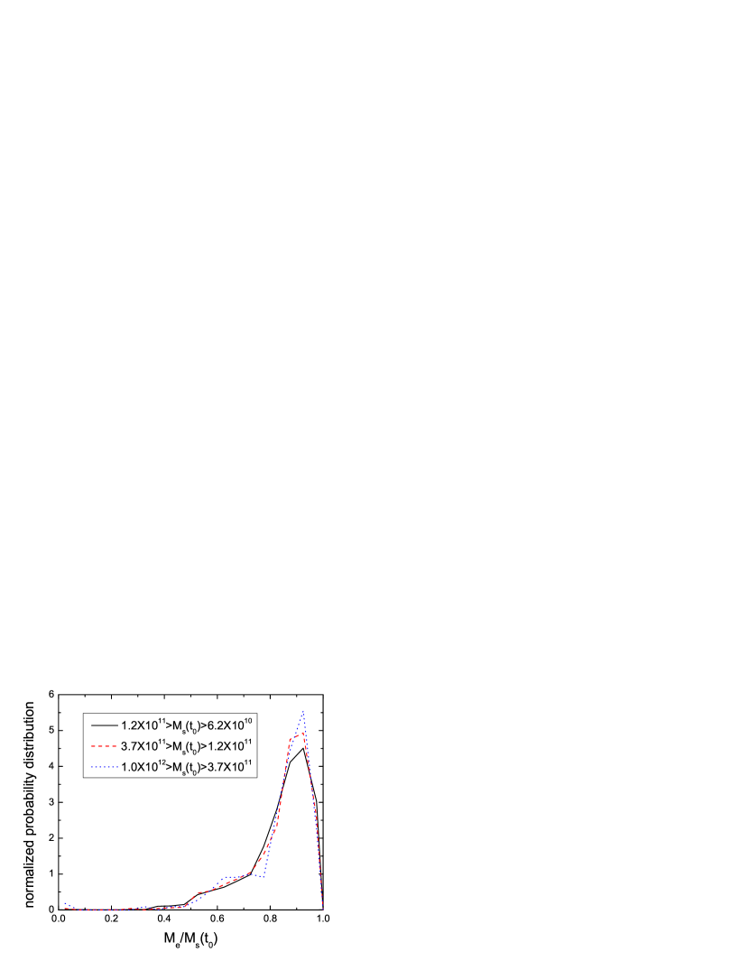
Figure 2: The probability distribution of $M_{\rm e}/M_{\rm s}(t_{0})$ for ejected subhalos in three mass bins, as indicated. Masses are in units of $h^{-1}{\rm M}_{\odot}$. See text for the definition of $M_{\rm e}$.

It is possible that an ejected subhalo after ejection can exchange mass with nearby halos or with the background density field, so that some of the particles contained in the ejected subhalo at the present time may not be contained in its ‘host’ halo. In order to quantify this, we consider an ejected mass, $M_{\rm e}$, which is defined as the mass of particles which are contained both in the ejected subhalo at $z=0$ and in its ‘host’ halo at the ejection redshift. The ratio between $M_{\rm e}$ and $M_{\rm s}(t_{0})$ can then be used as a measure of the fraction of retained mass of an ejected subhalo. In Fig. 2 we show the probability distribution of $M_{\rm e}/M_{\rm s}(t_{0})$. As one can see, most of the ejected subhalos at $z=0$ can retain more than $70\%$ of their original masses at ejection. This also shows that our method for identifying ejected subhalos is valid, in the sense that most of their masses were indeed once contained in their hosts.

2.3 Halo assembly times

We define the assembly redshift, $z_{\rm f}$, of a halo at redshift $z=0$ as the redshift when its most massive progenitor first reaches half of the final mass of the halo. If necessary, interpolation between two adjacent outputs is used. Here we do not use the merging tree described above to search for the progenitor. Instead we use the method described in Wang et al. (2007; see also Hahn et al. 2008). Very briefly, a halo in any given output at $z>0$ is considered to be a progenitor of the halo at $z=0$ if more than half of its particles are found in the final halo. In most cases, the merging trees constructed with this method is very similar to that constructed with the method described above. The advantage of the method adopted here is that it can trace an ejected subhalo backwards to the time even before it is accreted by its host halo. Since ejected halos may be strongly stripped by their host halos and lose part of their masses, the assembly redshifts of the ejected subhalos are generally higher than than their ejection redshifts and can be identified with this method.

3 The relationship between ejected subhalos and their hosts

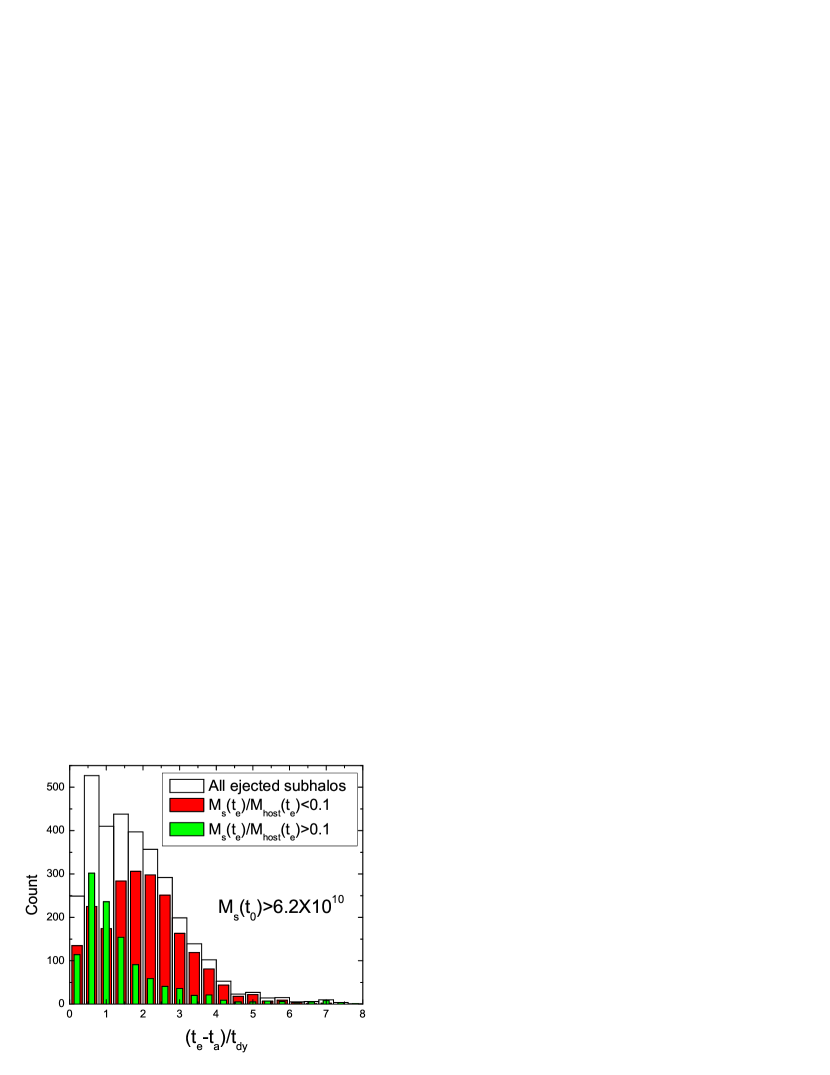
Figure 3: The histograms for $(t_{\rm a}-t_{\rm e})/t_{\rm dy}$ of ejected subhalos. The white histograms show the result for ejected subhalos with masses $M_{\rm s}(t_{0})>6.2\times 10^{10}h^{-1}{\rm M}_{\odot}$. And red and green hisograms show the results for two subsample indicated in the panel.

In Fig. 3, we show the histograms of the scaled time period an ejected subhalo stayed in its host: $(t_{\rm e}-t_{\rm a})/t_{\rm dy}$. Here $t_{\rm dy}$ is the dynamical time at $r_{200}$ of each host halo at the ejection time, with $r_{200}$ the virial radius within which the mean overdensity of the halois 200 times the critical density. The dynamical time is defined as:

$$t_{\rm dy}=\frac{r_{200}(t_{\rm e})}{v_{200}(t_{\rm e})}=\frac{1}{10H(t_{\rm e})}\,,$$ (1)

where $v_{200}$ is the circular velocity at $r_{200}$ and $H(t_{\rm e})$ is the Hubble constant, at the ejection time. As one can see, the time period an ejected subhalo stays within its host ranges from $<0.5$ to $>4$ times the dynamical time. To examine this time period in more detail, we split the ejected subhalos sample into two subsamples according to the $M_{\rm s}(t_{\rm e})/M_{\rm host}(t_{\rm e})$ ratio. The red (dark) and green (light) histograms in Fig. 3 represent the results with $M_{\rm s}(t_{\rm e})/M_{\rm host}(t_{\rm e})<0.1$ and $>0.1$, respectively. Evidently, the distribution for the case with $M_{\rm s}(t_{\rm e})/M_{\rm host}(t_{\rm e})<0.1$ is peaked around 2, and only 24% of halos have $(t_{\rm e}-t_{\rm a})/t_{\rm dy}<1$. On the other hand, halos with large $M_{\rm s}(t_{\rm e})/M_{\rm host}(t_{\rm e})$ ratio show quite a different distribution. It peaks at $\sim$ 0.6, and the fraction of halos with $(t_{\rm e}-t_{\rm a})/t_{\rm dy}<1$ is more than 55%. This indicates that many of the ejected subhalos with a large $M_{\rm s}(t_{\rm e})/M_{\rm host}(t_{\rm e})$ may be flybys which happen to be close to another halo and be linked to it by the FOF group finder. They may, therefore, represent a population that is different from the population with a small $M_{\rm s}(t_{\rm e})/M_{\rm host}(t_{\rm e})$, which most likely have run through their hosts. In what follows, we will treat these two populations separately. It should be pointed out, however, that there is an excess at 0.6 for halos with $M_{\rm s}(t_{\rm e})/M_{\rm host}(t_{\rm e})<0.1$, and there is a long tail for the subsample with $M_{\rm s}(t_{\rm e})/M_{\rm host}(t_{\rm e})>0.1$ (see Fig. 3). Thus, the $M_{\rm s}(t_{\rm e})/M_{\rm host}$ ratio alone cannot distinguish the two populations unambiguously.

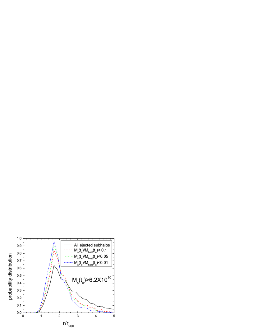
Figure 4: The probability distribution of ejected subhalos [with masses $M_{\rm s}(t_{0})>6.2\times 10^{10}h^{-1}{\rm M}_{\odot}$] in their distances to the host halos at $z=0$. The solid line shows the result for all ejected subhalos. The other lines show the results for the ejected halos with $M_{\rm s}(t_{\rm e})/M_{\rm host}(t_{\rm e})<0.1,0.05,0.01$ as indicated in the panel. The distance is scaled by $r_{200}$ of each host.

We show the probability distribution of ejected subhalos in their distances to the host halos at $z=0$ in Fig. 4. Here, the distance is scaled by $r_{200}$ of each host halo at redshift $z=0$. We use the scaled distance $r/r_{200}$ instead of $r$, because $r_{200}$ is the only important length scale related to the dynamics of a virialized halo. As one can see, the distribution peaks at $r/r_{200}\sim 1.6$. This is different from what is shown in L08, because their result includes also subhalos within host halos. Most of the ejected subhalos are distributed within $4r_{200}$, in good agreement with the finding of L08, but the distribution has a long tail at large distance. Our detailed examination shows that the long tail is dominated by ejected subhalos that have masses not much smaller than those of their ‘hosts’ at ejection. If we exclude the ejected subhalos with $M_{\rm s}(t_{\rm e})/M_{\rm host}(t_{\rm e})>\mu$, then the extended tail disappears as long as $\mu$ is chosen to be smaller than $0.1$. The distribution obtained for $\mu=0.1$, $0.05$ and $0.01$ are shown in Fig.4 for comparison. This result indicates that the two populations of the ejected subhalos discussed above have different distribution. Ludlow et al.(2008) found that subhalos with small mass at accretion time is less centrally concentrated than their massive counterparts. We do not find any significant evidence for such dependence. The difference in the result may be due to the difference in the halo definition and, particularly, in the contamination of the flybys population found in our simulation. This flyby population may be not important in L08 because of their way of selecting halos (see section 2.2 in their paper).

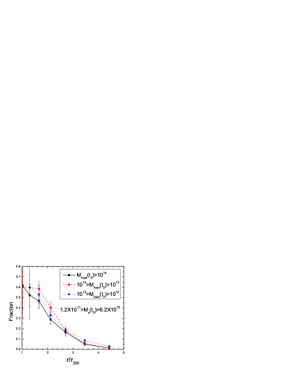
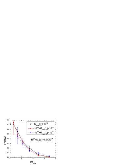
Figure 5: The ratio between the number of ejected subhalos and that of the total population (ejected plus normal) as a function of the distance to the hosts in various mass ranges. All masses are in $h^{-1}{\rm M}_{\odot}$. The distance is scaled by $r_{200}$ of each host.

Ejected subhalos in general are distributed around massive halos, but there are also normal halos which are distributed near massive halos but have never been inside a massive halo. In Fig. 5, we show the average fraction of ejected subhalos around their host halos. This is the ratio between the number of ejected subhalos and that of the total population (ejected plus normal) as a function of the scaled distance to the host halos. The left panel shows the average fractions of ejected subhalos with $6.2\times 10^{10}<M_{\rm s}(t_{0})<1.2\times 10^{11}\,h^{-1}{\rm M_{\odot}}$ around host halos in three mass ranges. In the right panel, we show the results for ejected subhalos with $1.2\times 10^{11}<M_{\rm s}(t_{0})<10^{12}\,h^{-1}{\rm M_{\odot}}$. In the mass ranges probed here, the ejected fraction as a function of the scaled distance is insensitive to the masses of both the ejected subhalos and the host halos. The fraction is between 30% and 75% in the range $r_{200}<r<2r_{200}$ and between 10% and 40% in the range $2r_{200}<r<3r_{200}$. These results are in agreement with those of L08, who found fractions of about 65% and 33% in the similar distance ranges (see also Gill et al. 2005; Wang et al. 2005), although the mass ranges for both the host halo and the ejected subhalos considered by them are quite different from what we are considering here. Note that, at large scaled distances, the fraction of ejected subhalos around host halos with the lowest mass is larger than that around massive host halos. This is again due to the population in which the ejected subhalos have masses comparable to their hosts at the time of ejection.

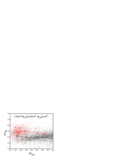
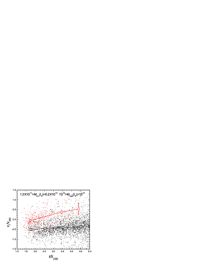
Figure 6: Radial velocity versus distance to the host halo for both ejected subhalos (red) and normal halos (black) in the mass ranges as indicated in the panels (all masses are in $h^{-1}{\rm M}_{\odot}$). The left panel shows halos around host halos with masses above $10^{13}\,h^{-1}{\rm M_{\odot}}$ and the right panel shows those around hosts with masses between $10^{13}\,h^{-1}{\rm M_{\odot}}$ and $10^{12}\,h^{-1}{\rm M_{\odot}}$. The symbols with error bars show the average radial velocities in different radius bins for both ejected subhalos (red circles) and normal halos (black squares). Note that the radial velocity shown here is the peculiar velocity relative to the host.

In Fig. 6 we show the scaled radial velocity, $v_{\rm r}/v_{200}$, versus scaled distance for both ejected and normal halos within $5\times r_{200}$ of the host halos of ejected halos. Here $v_{200}$ is the circular velocity of each host halo, and $v_{\rm r}$ is the relative peculiar velocity along the separation between a host and an ejected or a normal halo. We also split the ejected subhalos and normal halos into four subsamples according to the scaled distance and calculate the average velocity and average distance for each subsample. The results are shown as the big symbols in the figure. We consider two mass ranges of host halos, $M_{\rm host}>10^{13}\,h^{-1}{\rm M_{\odot}}$ and $10^{13}>M_{\rm host}>10^{12}\,h^{-1}{\rm M_{\odot}}$. Note that some normal halos may be counted more than once since they may be within $5\times r_{200}$ of more than one host halo. Clearly, the ejected subhalos and normal halos show different distribution in the phase space. The radial velocity distribution of ejected subhalos associated with massive hosts is quite symmetric and quite independent of the distance to the hosts, suggesting that on average there is about equal chance for an ejected subhalo to be moving away from or falling back towards the host. It is also consistent with the results of L08 although the velocities shown in their paper are the peculiar velocities plus the Hubble flow. The average radial velocity of ejected halos associated with low-mass hosts increase with the distance to the hosts. This is because of the contamination of the flybys mentioned above. The behavior of normal halos is quite different. Most of the normal halos are preferentially moving towards the host halos, as indicated by the systematically negative values of $v_{\rm r}$. The average value of $v_{\rm r}/v_{200}$ is about $-0.5$, independent on the distance and the mass of the hosts. The difference here suggests that the ejected subhalos are a distinctive population among the total halo population. A careful search shows that the scaled velocity dispersion of normal halos around small host halos is larger than that around massive host halos. This may be due to the fact that environmental effects play a more important role around smaller hosts.

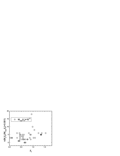
Figure 7: The relationship between the number of ejected subhalos and the assembly redshift of host halos. The left panel shows the number of ejected subhalos with $M_{\rm s}(t_{0})/M_{\rm host}(t_{0})>0.00031$ and the right panel show the results with $M_{\rm s}(t_{0})/M_{\rm host}(t_{0})>0.001$. The masses of host halos are larger than $10^{14}\,h^{-1}{\rm M_{\odot}}$.

Gao et al. (2004) find that the abundance of subhalos within host halos decreases with the formation redshift of the hosts, indicating that subhalos in early-formed host halos are more likely to be disrupted. However, as pointed out by L08, the subhalos within a host halo represent a rather incomplete census of the substructure physically related to the host. It is thus important to check whether the abundance of the ejected subhalos is also related to the assembly time of their hosts. In Fig. 7, we show the number of ejected subhalos as a function of the assembly redshift of the host halo. The left panel is the result for host halos with $M_{\rm host}(t_{0})>10^{14}\,h^{-1}{\rm M_{\odot}}$ and $M_{\rm s}(t_{0})/M_{\rm host}(t_{0})>0.00031$. As one can see, there is a clear trend that older host halos tend to eject more subhalos, although the scatter is quite large. To compare with Gao et al. (2004), we also show the results with $M_{\rm s}(t_{0})/M_{\rm host}(t_{0})>0.001$ in the right panel of Fig.7. The trend is weaker, likely due to the statistical variation caused by small numbers. This trend suggests that the old host halos tend not only to destroy their subhalos, but also to eject them. The decrease of subhalo abundance with formation redshift observed by Gao et al. (2004) is therefore a result of both subhalo ejection and destruction. For each host, the number of destroyed subhalos, $N_{\rm d}$, reads,

$$N_{\rm d}=N_{\rm a}-(N_{\rm s}+N_{\rm e})\,,$$ (2)

where $N_{\rm a}$ is the number of total accreted subhalos, and $N_{\rm s}$ and $N_{\rm e}$ are the numbers of surviving subhalos within the host and of ejected subhalos, respectively. Thus, in order to quantify the importance of ejection and destruction, one needs detailed merging trees to trace the evolution of subhalos within their hosts.

4 The origin of assembly bias

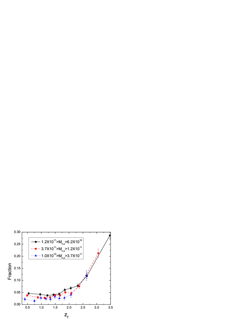
Figure 8: The fraction of ejected halos as a function of assembly redshift. All masses indicated in the panel are in $h^{-1}{\rm M}_{\odot}$.

Due to the strong interaction with their hosts before ejection, ejected subhalos may lose part of their mass. Since it is difficult for them to accrete more mass after ejection, the ejected subhalos should have acquired most of their mass before the ejection. Thus, on average these halos should have assembly times (defined in Section 2.3) that are earlier than their normal counterparts. In order to show this, we first split the halo sample in a certain mass range into 10 equal-sized subsamples according to assembly redshift. We then calculate the fraction of ejected halos and the average assembly redshift for each of these subsamples and show the fraction versus the redshift in Fig. 8. Among the 10 percent halos with the highest assembly redshifts, about $12\%$ to $27\%$ are ejected subhalos depending on the subhalo mass in question. The fraction decreases rapidly down to about $2\%$ - $5\%$ for halos with the lowest assembly redshifts. Since the ejected subhalos are expected to be located in high-density regions due to their associations with massive halos, they are expected to be strongly clustered. The presence of this population of ejected subhalos may therefore contribute to the assembly bias seen in cosmological $N$-body simulations (e.g. Gao et al. 2005; Jing, Suto & Mo 2007).

In order to examine whether or not the ejected subhalos are fully responsible for the assembly bias, we estimate the halo bias as a function of assembly redshift separately for all halos, normal halos and ejected (sub)halos. We first estimate the mean overdensity of dark matter within a sphere of radius $R$ around each dark matter halo, $\delta_{h}(R)$, and then measure the bias parameter of a given set of halos using

$$b=\frac{\langle\delta_{h}(R)\rangle}{\langle\delta_{m}(R)\rangle}\,,$$ (3)

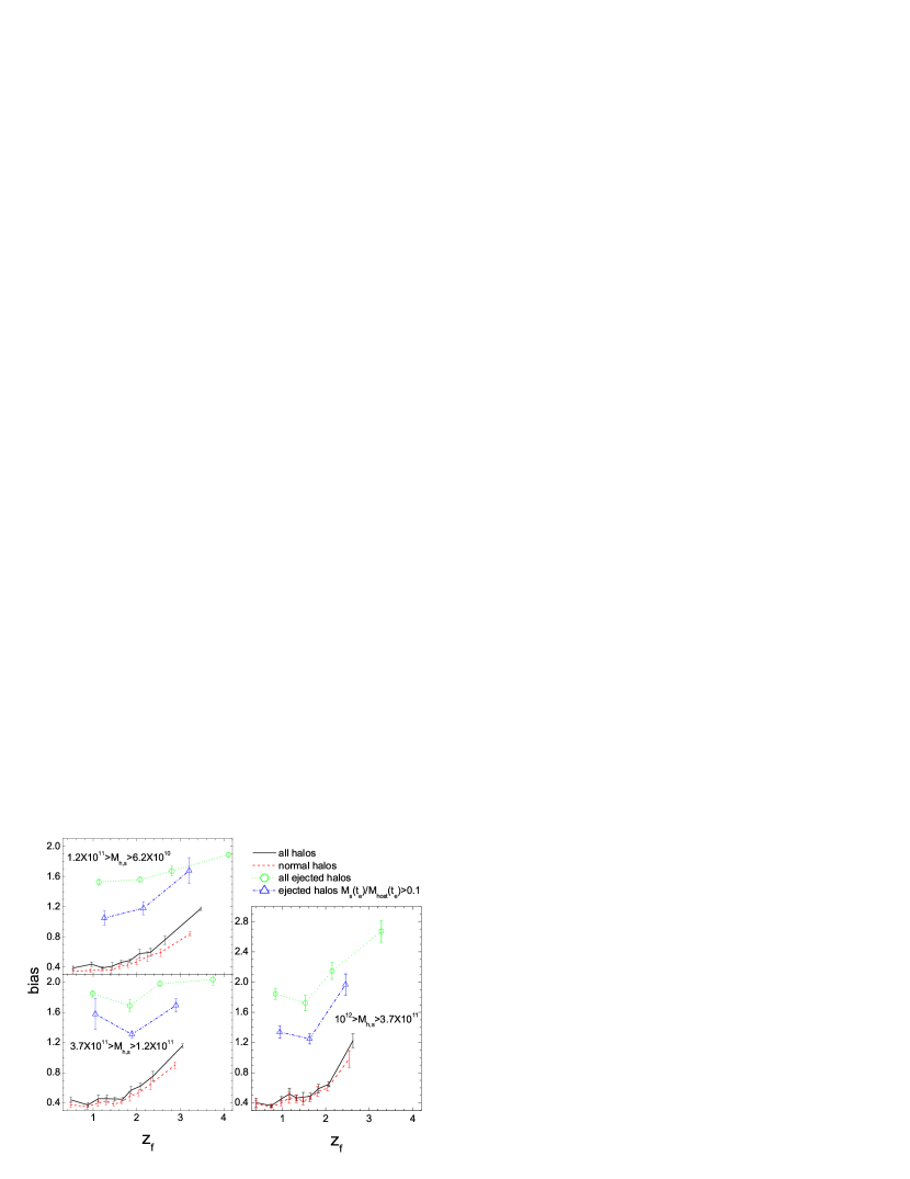
Figure 9: Halo bias as a function of assembly redshift for all halos (black solid lines), normal halos (red dash lines), and ejected subhalos (green dot lines). All masses indicated are in units of $h^{-1}{\rm M}_{\odot}$.

where $\langle\delta_{h}(R)\rangle$ is the average overdensity around the set of halos in question, and $\langle\delta_{m}(R)\rangle$ is the average overdensity within all spheres of radius $R$ centered on dark matter particles. This method has been demonstrated to reproduce the bias obtained using auto-correlation function of halos (Wang et al. 2007). The results are shown in Fig.9. As expected, the ejected subhalos in general have a much higher bias parameter than other halos of similar masses. The bias parameter for ejected subhalos with $M_{\rm s}(t_{\rm e})/M_{\rm host}(t_{\rm e})>0.1$ is lower (blue dash dot lines), presumably because they are associated with hosts of lower masses, as mentioned above. However, even if all ejected subhalos are excluded, the assembly bias is still significant (see the red dash lines in Fig. 9). For halos with masses larger than $10^{11.5}h^{-1}{\rm M}_{\odot}$, the assembly bias is almost entirely due to normal halos instead of ejected subhalos. Even for halos of lower masses (e.g. $\sim 10^{11}h^{-1}{\rm M}_{\odot}$), including ejected only increases the bias parameter by $50\%$. The reason is that the fraction of ejected subhalos is small among the total halo population of the same mass. Thus, ejected subhalos cannot explain the full range of assembly bias seen in cosmological $N$-body simulations, even though they are strongly clustered in space. This result is consistent with the finding of Wang et al. (2007) that the assembly bias is mainly due to the fact that small old halos tend to live in the vicinity of massive halos and their growth at low redshift is suppressed by the large-scale tidal field. An analysis along this line is performed by Keselman & Nusser (2007). They used the punctuated Zel’dovich approximation, in which the highly non-linear effects such as tidal stripping are excluded, to run simulations of structure formation, and found that the assembly bias is still present. All these indicate that the large-scale environmental effects have also played an important role in the formation of some normal halos (see also Hahn et al. 2008).

5 Summary and discussion

In this paper, we use a high-resolution cosmological simulation to study the distribution of the ejected subhalos, their connection to the host halos, and their contribution to the halo assembly bias seen in cosmological simulations. Our main results are summarized as follows.

1. The fraction of the ejected subhalos in the total halo population of the same mass ranges from 9% to 4% for halo masses from $\sim 10^{11}$ to $\sim 10^{12}\,h^{-1}{\rm M_{\odot}}$.

2. The time period an ejected subhalo stays in its host has wide distribution, ranging from less than 0.5 to more than 4 times the dynamical time of of the host. The distribution peaks at 2 and 0.6 for ejected subhalos with $M_{\rm s}(t_{\rm e})/M_{\rm host}(t_{\rm e})<0.1$ and $>0.1$, respectively, indicating the existence of two distinctive populations of ejected halos.

3. Most of the ejected subhalos are found to be distributed within about 4 times the virial radius of their hosts. The fraction of ejected subhalos is about 30% - 75% within the distance range between $r_{200}$ and $2r_{200}$ to the hosts and about 10% - 40% in the distance range $2r_{200}<r<3r_{200}$.

4. The radial velocity distribution of ejected subhalos is quite symmetric, while normal halos of the same mass generally tend to fall onto nearby massive halos.

5. The number of subhalos ejected from a host of given mass increases with the assembly redshift of the host. Thus, subhalos tend to be less abundant in halos that formed earlier, not only because subhalos in such hosts are more likely to be destroyed, but also because they are more likely to be ejected.

6. Ejected subhalos in general reside in high-density regions, and have a much higher bias parameter than normal halos of the same mass. They also have earlier assembly times, so that they contribute to the assembly bias of dark matter halos seen in cosmological simulations.

7. The assembly bias is not dominated by the ejected population. This indicates that large-scale environmental effects may also be important in the formation of normal halo population, and in producing the assembly bias.

The results obtained here may have important implications to the understanding of galaxy distribution in the cosmic density field. As a subhalo pass through a massive host, tidal and/or ram-pressure stripping by the host halo may get rid of the gas reservoir in the ejected halo, thereby quenching star formation in it. The situation may be similar to what happens to satellite galaxies, although the ejected galaxies are not observed as satellites in massive halos. If the quenching processes are effective, we would expect a population of faint red galaxies that are not contained in any massive halos but are distributed around them. It is therefore interesting to see if such a population of galaxies does exist. In a recent investigation, Wang et al. (2008) found that the reddest $15$ - $20\%$ among all faintest galaxies are physically associated with massive halos. About half of this population resides within massive halos as satellites. The other half resides outside massive halos and are distributed within about 3 times the virial radii of their nearest massive halos. Very likely, this population of galaxies are hosted by the ejected subhalos we are studying here. Clearly, it is interesting to study further the connection between ejected subhalos and this population of galaxies, so as to understand how environmental effects operate on satellite galaxies in their host halos.

References

- Bardeen et al. (1986) Bardeen J. M., Bond J. R., Kaiser N., Szalay A. S., 1986, ApJ, 304, 15
- Bett et al. (2007) Bett P., Eke V., Frenk C. S., Jenkins A., Helly J., Navarro J., 2007, MNRAS, 376, 215
- Dalal et al. (2008) Dalal N., White M., Bond J. R., Shirokov A., 2008, arXiv, arXiv:0803.3453
- Desjacques (2008) Desjacques V., 2008, MNRAS, 388, 638
- Gao et al. (2004) Gao L., White S. D. M., Jenkins A., Stoehr F., Springel V., 2004, MNRAS, 355, 819
- Gao, Springel, & White (2005) Gao L., Springel V., White S. D. M., 2005, MNRAS, 363, L66
- Gao & White (2007) Gao L., White S. D. M., 2007, MNRAS, 377, L5
- Gill, Knebe, & Gibson (2005) Gill S. P. D., Knebe A., Gibson B. K., 2005, MNRAS, 356, 1327
- Hahn et al. (2008) Hahn O., Porciani C., Dekel A., Carollo C. M., 2008, arXiv, arXiv:0803.4211
- Harker et al. (2006) Harker G., Cole S., Helly J., Frenk C., Jenkins A., 2006, MNRAS, 367, 1039
- Jing (1998) Jing Y. P., 1998, ApJ, 503, L9
- Jing, Mo, & Boerner (1998) Jing Y. P., Mo H. J., Boerner G., 1998, ApJ, 494, 1
- Jing & Suto (2002) Jing Y. P., Suto Y., 2002, ApJ, 574, 538
- Jing, Suto, & Mo (2007) Jing Y. P., Suto Y., Mo H. J., 2007, ApJ, 657, 664
- Keselman & Nusser (2007) Keselman J. A., Nusser A., 2007, MNRAS, 382, 1853
- Li, Mo, & Gao (2008) Li Y., Mo H. J., Gao L., 2008, MNRAS, 389, 1419
- Lin, Jing, & Lin (2003) Lin W. P., Jing Y. P., Lin L., 2003, MNRAS, 344, 1327
- Ludlow et al. (2008) Ludlow A. D., Navarro J. F., Springel V., Jenkins A., Frenk C. S., Helmi A., 2008, arXiv, arXiv:0801.1127
- Maulbetsch et al. (2007) Maulbetsch C., Avila-Reese V., Colín P., Gottlöber S., Khalatyan A., Steinmetz M., 2007, ApJ, 654, 53
- Mo, Jing, & Börner (1997) Mo H. J., Jing Y. P., Borner G., 1997, MNRAS, 286, 979
- Mo, Jing & White (1997) Mo H. J., Jing Y. P., White S. D. M., 1997, MNRAS, 284, 189
- Mo & White (1996) Mo H. J., White S. D. M., 1996, MNRAS, 282, 347
- Peacock & Smith (2000) Peacock J. A., Smith R. E., 2000, MNRAS, 318, 1144
- Sandvik et al. (2007) Sandvik H. B., Möller O., Lee J., White S. D. M., 2007, MNRAS, 377, 234
- Sheth, Mo, & Tormen (2001) Sheth R. K., Mo H. J., Tormen G., 2001, MNRAS, 323, 1
- Sheth & Tormen (1999) Sheth R. K., Tormen G., 1999, MNRAS, 308, 119
- Seljak & Warren (2004) Seljak U., Warren M. S., 2004, MNRAS, 355, 129
- Wang et al. (2005) Wang H. Y., Jing Y. P., Mao S., Kang X., 2005, MNRAS, 364, 424
- Wang, Mo, & Jing (2007) Wang H. Y., Mo H. J., Jing Y. P., 2007, MNRAS, 375, 633
- Wang et al. (2008) Wang Y., Yang X., Mo H. J., van den Bosch F. C., katz N., Pasquali A., McIntosh D. H., Weinmann S. M., 2008, arXiv, arXiv:0812.3723
- Wechsler et al. (2006) Wechsler R. H., Zentner A. R., Bullock J. S., Kravtsov A. V., Allgood B., 2006, ApJ, 652, 71
- Wetzel et al. (2007) Wetzel A. R., Cohn J. D., White M., Holz D. E., Warren M. S., 2007, ApJ, 656, 139
- Yang, Mo, & van den Bosch (2003) Yang X., Mo H. J., van den Bosch F. C., 2003, MNRAS, 339, 1057
- Zhu et al. (2006) Zhu G., Zheng Z., Lin W. P., Jing Y. P., Kang X., Gao L., 2006, ApJ, 639, L5