Direct observation of Hardy’s paradox by joint weak measurement with an entangled photon pair

Abstract

We implemented a joint weak measurement of the trajectories of two photons in a photonic version of Hardy’s experiment. The joint weak measurement has been performed via an entangled meter state in polarization degrees of freedom of the two photons. Unlike Hardy’s original argument in which the contradiction is inferred by retrodiction, our experiment reveals its paradoxical nature as preposterous values actually read out from the meter. Such a direct observation of a paradox gives us new insights into the spooky action of quantum mechanics.

Although it is natural to ask what is the value of a physical quantity in the middle of a time evolution, it is difficult to answer such a question in quantum mechanics, especially when post-selection is involved. Hardy’s thought experiment [1] is a typical example in which we encounter such a difficulty. Figure 1(a) shows a photonic version of the experiment, which was demonstrated by Irvine et al. recently [2]. The scheme consists of two Mach-Zehnder interferometers MZ1 and MZ2 with their inner arms ($O_{1}$, $O_{2}$) overlapping on each other at the 50:50 beam splitter BS3. If photons 1 and 2 simultaneously arrive at BS3, due to a two-photon interference effect, they always emerge at the same port. This corresponds to the positron-electron annihilation in the original thought experiment [1]. The path lengths of MZ1 are adjusted so that photon 1 should never appear at $C_{1}$ by destructive interference, when photon 2 passes the outer arm $NO_{2}$ and thus has no disturbance on MZ1. The path lengths of MZ2 are adjusted similarly. Then, a coincidence detection at $C_{1}$ and $C_{2}$ gives a paradoxical statement on which paths the detected photons have taken. The detection at $C_{1}$ ($C_{2}$) implies that MZ1 (MZ2) has been disturbed by photon 2 (1) travelling along $O_{2}$ ($O_{1}$). We may thus infer that the conditional probabilities satisfy

$$P(O_{1}|C_{1}C_{2})=P(O_{2}|C_{1}C_{2})=1.$$ (1)

On the other hand, if both photons had taken the inner arms, the coincidence detection would have never happened due to the two photon interference. Hence we infer that

$$P(O_{1}O_{2}|C_{1}C_{2})=0.$$ (2)

The two inferred statements are apparently contradictory to each other, which is the well-known Hardy’s paradox.

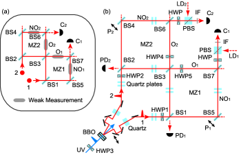
Figure 1: Experimental setup for Hardy’s paradox. (a) The photonic version of Hardy’s thought experiment. Each of the MZ interferometers MZ1 and MZ2 is composed of four 50:50 beam splitters (BS). (b) The schematics of the experiment with joint weak measurement. Entangled photon pairs are generated via spontaneous parametric down-conversion from a pair of type I phase matched 2mm thick BBO crystal [17] pumped by a UV pulse (a central wave length 395nm and an average power 180mW). The UV pulse is taken from the frequency doubled Ti:sapphire laser (wavelength, 790nm; pulse width, 140fs; repetition rate, 76MHz). Quartz crystals are used to compensate the group velocity mismatch and adjust the relative phase between horizontal and vertical polarization state. Polarization dependent phase shifts in MZs are compensated by quartz plates in the MZs so that MZs give the same phase shifts to any polarization state. Extra laser diodes (LDs) and photo diodes (PDs) are used for adjusting and stabilizing the optical lengths of MZs via piezo stage (Ps). The photons are detected by photon detectors (Cs). The observed visibility of two photon interference at BS3 was 97.8 $\pm$ 0.3% for horizontally polarized photons.

One may argue that we should abandon the attempt to address the question itself, on the ground that the trajectory of photons cannot be measured without utterly changing the time evolution. But this reasoning is not necessarily true if we are allowed to repeat the same experiment many times. Aharonov et al. has proposed weak measurement [3, 4], in which a measurement apparatus (meter) interacts with the system to be measured so weakly that the state of the system is not significantly disturbed. The readout of the meter from a single run of experiment may be subtle and noisy, but by taking the average over many runs we can correctly estimate the expectation value of the measured observable, $\langle\psi\,|\hat{A}|\,\psi\rangle$, when the initial state of the measured system is $|\,\psi\rangle$. In this setup, we may ask what is the averaged readout over the runs in which the system is finally found to be in a state $|\,\phi\rangle$. In the limit of no disturbance, this gives an operational way of defining what is the value of $\hat{A}$ at the middle of a time evolution from $|\,\psi\rangle$ to $|\,\phi\rangle$, and is found to be given by the real part of the following expression

$$\hat{A}_{\bf w}\equiv\langle\phi|\hat{A}|\psi\rangle/\langle\phi|\psi\rangle,$$ (3)

which is called the weak value of $\hat{A}$. So far, related interesting features were discussed [5, 6, 7, 8, 9, 10, 11] and experimental observations of weak values were reported [12, 13, 14, 15, 16].

Suppose that weak measurements of trajectories are applied to Hardy’s experiment at the shaded regions in Fig. 1(a). The state of the photons entering these regions is $|\psi\rangle=(|NO_{1}\rangle|O_{2}\rangle+|O_{1}\rangle|NO_{2}\rangle+|NO_{1}\rangle|NO_{2}\rangle)/\sqrt{3}$, and the coincidence detection retrodicts the state leaving the regions to be $|\phi\rangle=(|NO_{1}\rangle-|O_{1}\rangle)(|NO_{2}\rangle-|O_{2}\rangle)/2$ [8]. Then the weak values can be calculated to be

$$|O_{1},O_{2}\rangle\langle O_{1},O_{2}|_{\bf w}=0,\ |NO_{1},NO_{2}\rangle\langle NO_{1},NO_{2}|_{\bf w}=-1,$$

$$|O_{1},NO_{2}\rangle\langle O_{1},NO_{2}|_{\bf w}=1,\ |NO_{1},O_{2}\rangle\langle NO_{1},O_{2}|_{\bf w}=1.$$ (4)

The first equation implies Eq. (2) holds. We also see that Eq. (1) holds since, for instance, $|O_{1}\rangle\langle O_{1}|_{\bf w}=|O_{1},O_{2}\rangle\langle O_{1},O_{2}|_{\bf w}+|O_{1},NO_{2}\rangle\langle O_{1},NO_{2}|_{\bf w}=1$. Hence the readout of the meter is indeed consistent with both of the naively inferred conditions (1) and (2). The reason why these two contradictory conditions are satisfied at the same time can now be ascribed to the appearance of a negative value, $|NO_{1},NO_{2}\rangle\langle NO_{1},NO_{2}|_{\bf w}=-1$. It implies that the average readout over post-selected events falls on a value that never appears if no post-selection is involved.

In this paper, we report an experimental demonstration of weak measurements applied to Hardy’s experiment. Since the observables to be measured are of path correlations between the two photons, we need to implement a joint weak measurement that can extract such correlations. Although a number of schemes for joint weak measurement have been proposed [18, 19], here we propose the most intuitive approach using meter qubits initially prepared in an entangled state. We conducted measurements with varied strength, and confirmed that it works properly when each photon is injected to a fixed arm. We also measured the visibility of the interferometers to verify that the disturbance vanishes in the limit of weak measurement. Then we conducted Hardy’s experiments and observed that, as the measurement became weaker, three readouts moved toward the conditions (1) and (2) while another readout went to negative.

Let us first introduce our scheme of joint weak measurement for two qubits in a general setting. Let $\{|\,0\rangle,|\,1\rangle\}$ be the standard basis of a qubit. For weak measurement of the observable $|\,0\rangle\langle 0\,|$ of a qubit, one can prepare another qubit in a suitable state and apply a controlled-NOT (C-NOT) gate between the two qubits [14]. Here we want to carry out weak measurements of observables $|\,kl\rangle_{s_{1}s_{2}}\langle kl\,|$ $(k,l=0,1)$ for the two signal qubits, $s_{1}$ and $s_{2}$, and we may use two meter qubits, $m_{1}$ and $m_{2}$, and apply two C-NOT gates in parallel. The signal (meter) qubit corresponds to the control (target) qubit and the meter qubit is flipped when the signal qubit is in $|1\rangle$. Note that in our implementation of Hardy’s experiment, the photon path corresponds to the signal qubit and its polarization to the meter qubit. We found that the desired weak measurements are achieved by a simple choice of the initial state of the meter qubits,

$$|\xi\rangle_{m} = \delta|00\rangle_{m_{1}m_{2}}+\varepsilon(|01\rangle_{m_{1}m_{2}}+|10\rangle_{m_{1}m_{2}}+|11\rangle_{m_{1}m_{2}})$$ (5)

$$= (\delta-\varepsilon)|00\rangle_{m_{1}m_{2}}+\varepsilon\sum_{kl}|kl\rangle_{m_{1}m_{2}},$$

where $\delta^{2}+3\varepsilon^{2}=1$ and $\delta\geq\varepsilon\geq 0$. When the signal qubits are in $|\psi\rangle_{s}=\sum_{ij}c_{ij}|ij\rangle_{s_{1}s_{2}}$, the application of the parallel C-NOT operation $U_{sm}$ results in

$$U_{sm}|\psi\rangle_{s}|\xi\rangle_{m}$$ (6)

$$= \sum_{ij}c_{ij}|ij\rangle_{s_{1}s_{2}}[(\delta-\varepsilon)|ij\rangle_{m_{1}m_{2}}+\varepsilon\sum_{kl}|kl\rangle_{m_{1}m_{2}}]$$

$$= \sum_{kl}[(\delta-\varepsilon)|kl\rangle_{s_{1}s_{2}}\langle kl|+\varepsilon]|\psi\rangle_{s}|kl\rangle_{m_{1}m_{2}}.$$

The meter qubits will then be measured in the basis $\{|\,kl\rangle_{m_{1}m_{2}}\}$ to produce an outcome $(k,l)$. If the signal qubits are in state $|ij\rangle_{s_{1}s_{2}}$ initially, the probability $P_{m}(k,l)$ of outcome $(k,l)$ becomes

$${P}_{m}(k,l)=\left\{\begin{array}[]{ll}\delta^{2}&((k,l)=(i,j))\\ \varepsilon^{2}&((k,l)\neq(i,j)).\end{array}\right.$$ (9)

We see that the outcome $(i,j)$, corresponding to the state of the signal, has a larger probability than the others. The contrast $\delta^{2}-\varepsilon^{2}$ will be regarded as the measurement strength. When $\delta^{2}-\varepsilon^{2}=1$ $(\delta=1,\varepsilon=0)$, this scheme gives a projection measurement (strong measurement) on the signal qubits. Decreasing $\delta^{2}-\varepsilon^{2}$ makes the measurement weaker, and at $\delta^{2}-\varepsilon^{2}=0$ $(\delta=\varepsilon=1/2)$, the operation of $U_{sm}$ introduces no disturbance on the signal qubits (Appendix A). Let us introduce a normalized readout $R(k,l)$ by

$$R(k,l) \equiv [P_{m}(k,l)-\varepsilon^{2}]/(\delta^{2}-\varepsilon^{2}).$$ (10)

Then, regardless of the value of $\delta^{2}-\varepsilon^{2}>0$, we have $R(k,l)=1$ for $(k,l)=(i,j)$ and $R(k,l)=0$ otherwise. When the initial state of the signal qubits is $|\,\psi\rangle_{s}=\sum_{ij}c_{ij}|ij\rangle_{s_{1}s_{2}}$, the normalized readout becomes $R(k,l)=|c_{k,l}|^{2}$, which coincides with the expectation value $\langle|\,kl\rangle_{s_{1}s_{2}}\langle kl\,|\rangle$. Of course, for the estimation of $R(k,l)$ and hence of $P_{m}(k,l)$, we need to repeat the preparation of the initial state $|\,\psi\rangle_{s}$ and the measurement many times.

Now in a situation like Hardy’s experiment, we are interested in the readout of the meter on condition that the signal qubits are finally measured to be in state $|\,\phi\rangle_{s}$. From the definition (3), we have

$${}_{s}\langle\phi|U_{sm}|\psi\rangle_{s}|\xi\rangle_{m}$$ (11)

$$= \sum_{kl}[(\delta-\varepsilon)|kl\rangle_{s_{1}s_{2}}\langle kl|_{\bf w}+\varepsilon]_{s}\langle\phi|\psi\rangle_{s}|kl\rangle_{m}.$$

The conditional probability of the outcome $(k,l)$ is then given by

$${P}_{m}(k,l|\phi) = |(\delta-\varepsilon)|kl\rangle_{s_{1}s_{2}}\langle kl|_{\rm w}+\varepsilon|^{2}/[1-(\delta-\varepsilon)^{2}\zeta]$$ (12)

with $\zeta\equiv 1-\sum_{ij}||ij\rangle_{s_{1}s_{2}}\langle ij|_{\rm w}|^{2}$. The normalized readout is found to be

$$R(k,l|\phi)\equiv[{P}_{m}(k,l|\phi)-\varepsilon^{2}]/(\delta^{2}-\varepsilon^{2})$$

$$= \frac{2\varepsilon(\delta-\varepsilon){\rm Re}[|kl\rangle_{s_{1}s_{2}}\langle kl|_{\rm w}]+(\delta-\varepsilon)^{2}[||kl\rangle_{s_{1}s_{2}}\langle kl|_{\rm w}|^{2}+\varepsilon^{2}\zeta]}{(\delta^{2}-\varepsilon^{2})[1-(\delta-\varepsilon)^{2}\zeta]}$$

$$\to {\rm Re}[|kl\rangle_{s_{1}s_{2}}\langle kl|_{\rm w}]\ \ \ (\delta^{2}-\varepsilon^{2}\to 0).$$ (14)

We see that the normalized readout in the limit of no disturbance coincides with the real part of the weak value.

In our experiment, the signal qubit corresponds to the paths taken by the photon as $|\,0\rangle=|\,NO\rangle$ and $|\,1\rangle=|\,O\rangle$, whereas the meter qubit is assigned to the polarization of the same photon as $|\,0\rangle=|\,+\rangle$ and $|\,1\rangle=|\,-\rangle$, where $|\pm\rangle\equiv(|H\rangle\pm|V\rangle)/\sqrt{2}$ and $H/V$ is the horizontal/vertical polarization. The interferometers in Fig. 1(a) are constructed so that there is no polarization dependence, except for the shaded region where wave plates are placed to realize $U_{sm}$. The polarization dependence of the coincidence events is then analyzed to determine $P_{m}(k,l|\phi)$.

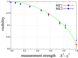
Figure 2: Relation between the visibility of MZ1(2) and the measurement strength. The solid curve represents the theoretically expected visibility, $2\varepsilon(\delta+\varepsilon)$.

The detail of the setup is shown in Fig. 1(b). We generate the photon pairs in a nonmaximally entangled state $\eta|HH\rangle_{12}+\bar{\eta}|VV\rangle_{12}$ from PDC, where $\eta^{2}+\bar{\eta}^{2}=1$ and $\eta$ and $\bar{\eta}$ are properly adjusted to be real numbers. The coefficients $\eta$ and $\bar{\eta}$, which can be tuned by HWP3, are determined by the ratio between the coincidence counts of $|HH\rangle$ and $|VV\rangle$. The state is transformed into $|\xi\rangle_{m}$ by rotating the polarization of two photons by half wave plates HWP1 and HWP2. The measurement strength is simply calculated by the measured $\eta$ and $\bar{\eta}$ and the angle of HWP1 and HWP2. After the photons pass through BS1, BS2 and BS3, the two-photon state is represented as $|\psi\rangle_{s}|\xi\rangle_{m}$. The C-NOT operations between signals and meters are simply performed by flipping the polarization as $|\pm\rangle\to|\mp\rangle$ via HWP4 and HWP5 in the overlapped arms, $O_{1}$ and $O_{2}$. The polarization basis ($|\,+\rangle,|\,-\rangle$) for the meter measurement is selected by HWP and PBS just before detectors $C_{1}$ and $C_{2}$. The coincidence counts, typically a few thousands, are accumulated over 5-12 min per basis to determine each $R(k,l|\phi)$. All error bars assume the Poisson statistics of the counts.

First we show the observed trade-off between the measurement strength and the visibilities of interference at MZ1 and MZ2. The measurements were done as follows: We blocked the arm $O_{2}$($O_{1}$) and recorded the coincidence detection at $C_{1}$ and $C_{2}$ by changing the path length via piezo stage P₁(P₂). In order to measure the polarization-independent visibilities, we measured the interference fringes in the states $|++\rangle$, $|+-\rangle$, $|-+\rangle$, and $|--\rangle$ independently and calculated the average visibility. The visibilities for various measurement strengths are shown in Fig. 2. We can clearly see that weakening the measurement makes the visibility larger (Appendix B).

We also show that our measurement gives proper values of the readouts $R(k,l|\phi)$ when the photons travel the fixed arms $|O_{1},NO_{2}\rangle,|NO_{1},O_{2}\rangle,$ and $|NO_{1},NO_{2}\rangle$. We blocked the arms of no interest and determined $R(k,l|\phi)$ from the coincidence detection on the basis { $|++\rangle$, $|+-\rangle$, $|-+\rangle$, $|--\rangle$ } . The experimental results are plotted in Fig. 3. In any measurement strength, the corresponding readout for the signal state is close to 1 and the other readouts are close to 0. This clearly shows the apparatus properly measures the trajectories of the photons. The systematic deviation from the expected values at small values of $\delta^{2}-\varepsilon^{2}$ is believed to be the results of very tiny misalignments of the axes of the wave plates. Such an enhancement is a feature of weak measurement and can be used for super-sensitive measurements as shown in [16].

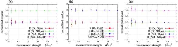
Figure 3: Experimental results when the initial states are in (a)$|O_{1},NO_{2}\rangle$, (b)$|NO_{1},O_{2}\rangle$, and (c)$|NO_{1},NO_{2}\rangle$.

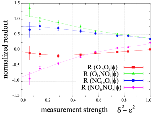
Figure 4: Observed readouts in Hardy’s experiment. The curves that roughly fit the data points are of a simple model of imperfections, and are only shown to guide the eye.

With this meter, we performed measurements of the trajectories of the photons in Hardy’s thought experiment. The observed readouts are shown in Fig. 4. Let us see the results around 0.3 measurement strength. The visibility above 0.9 shown in Fig. 2 suggests that the measurement is fairly weak, and the systematic deviation in Fig. 3 is small at this strength. For each of the photons, the readouts suggest a high probability of taking the overlapped arm: $R(O_{1}|\phi)\equiv R(O_{1},NO_{2}|\phi)+R(O_{1},O_{2}|\phi)=0.72\pm 0.09$ and $R(O_{2}|\phi)=0.53\pm 0.09$. Nonetheless, the readout for the joint probability is around zero, namely, $R(O_{1},O_{2}|\phi)=-0.18\pm 0.05$. We also see that $R(NO_{1},NO_{2}|\phi)=-0.43\pm 0.04$ takes a large negative value, which cannot be interpreted as a probability. Although the statistical and systematic errors are large around zero measurement strength, we see that $R(O_{1},NO_{2}|\phi)$, $R(NO_{1},O_{2}|\phi)$, $R(O_{1},O_{2}|\phi)$, and $R(NO_{1},NO_{2}|\phi)$ approach the expected weak values in Eq. (4) when the measurement strength goes to 0.

Let us emphasize here that our experimental results by themselves can elucidate the paradoxical nature of Hardy’s experiment, without any reference to the theory explaining how our measurement works. From the results in Fig. 3, we see that our measurement apparatus should properly give the probabilities on the trajectories of the photons, if such quantities ever exist. Then, in Hardy’s setup, the same measurement presents a contradictory statement in Fig. 4 that the probability of finding a photon in arm $O_{1}$ approaches 1 and so does the probability for arm $O_{2}$, whereas the joint probability of photons being in both of the arms stays at about 0. Moreover, the readout points to a negative value for the joint probability for arms $NO_{1}$ and $NO_{2}$. Unlike Hardy’s original argument, our demonstration reveals the paradox by observation, rather than inference.

We have experimentally demonstrated a joint weak measurement with an entangled photon pair and directly observed paradoxical results in Hardy’s thought experiment. Our demonstration clearly reproduces Hardy’s paradox in an experimentally accessible manner. Weak measurements have attracted attention due to the possibility of achieving small-backaction and high-sensitivity measurements by simple optical setups. We believe the demonstrated joint weak measurement is useful not only for exploiting fundamental quantum physics, but also for various applications such as quantum metrology and quantum information technology.

Note added. During the preparation of this manuscript, we came to know of a work by Lundeen and Steinberg [20], which has demonstrated similar results by using, interestingly, different methods for joint weak measurement and for constructing Hardy’s interferometer.

Appendix A

The positive operator valued measure (POVM) for the measurement on the signal qubits is given by

$$\hat{\Pi}_{kl} = \delta^{2}|kl\rangle_{s_{1}s_{2}}\langle kl|+\varepsilon^{2}\sum_{ij\neq kl}|ij\rangle_{s_{1}s_{2}}\langle ij|$$ (15)

$$= (\delta^{2}-\varepsilon^{2})|kl\rangle_{s_{1}s_{2}}\langle kl|+\varepsilon^{2}.$$

The same POVM can be realized also by a nonentangled initial state of the meter qubits, $\delta^{2}|00\rangle_{m_{1}m_{2}}\langle 00|+\varepsilon^{2}(|01\rangle_{m_{1}m_{2}}\langle 01|+|10\rangle_{m_{1}m_{2}}\langle 10|+|11\rangle_{m_{1}m_{2}}\langle 11|)$. This separable state of the meter qubits, however, fails to derive a joint weak value, because the signal qubits are utterly disturbed even if $\delta^{2}-\varepsilon^{2}=0$.

Appendix B

A general relation between the visibility $V$ and the measurement strength was discussed in [21]. It was shown that $V^{2}+K^{2}\leq 1$ holds, where $K\equiv 1-2p_{\rm err}$ stands for the measurement strength defined in terms of the error probability $p_{\rm err}$ in the which-path measurement. In our case, the initial marginal state of the meter qubit $m_{1}$ is a mixed state, which is, from Eq. (5), calculated to be a mixture of state $|\,\phi_{0}\rangle_{m_{1}}\equiv(\delta|\,0\rangle_{m_{1}}+\varepsilon|\,1\rangle_{m_{1}})/\sqrt{p_{0}}$ with probability $p_{0}\equiv\delta^{2}+\varepsilon^{2}$ and $|\,\phi_{1}\rangle_{m_{1}}\equiv(|\,0\rangle_{m_{1}}+|\,1\rangle_{m_{1}})/\sqrt{2}$ with $p_{1}\equiv 2\varepsilon^{2}$. The state $|\,\phi_{0}\rangle_{m_{1}}$ leads to a measurement strength $K_{0}=(\delta^{2}-\varepsilon^{2})/(\delta^{2}+\varepsilon^{2})$ and visibility $V_{0}=\sqrt{1-K_{0}^{2}}=2\varepsilon\delta/(\delta^{2}+\varepsilon^{2})$, whereas $|\,\phi_{1}\rangle_{m_{1}}$ leads to $K_{1}=0$ and $V_{1}=1$. Hence, on average, the measurement strength becomes $K_{\rm ave}\equiv p_{0}K_{0}+p_{1}K_{1}=\delta^{2}-\varepsilon^{2}$ and $V_{\rm ave}\equiv p_{0}V_{0}+p_{1}V_{1}=2\varepsilon(\delta+\varepsilon)$, which is shown as the solid curve in Fig. 3. Due to the mixture, the averaged values $K_{\rm ave}$ and $V_{\rm ave}$ do not saturate the general bound $V_{\rm ave}^{2}+K_{\rm ave}^{2}\leq 1$.

References

References

- [1] L. Hardy, Phys. Rev. Lett. 68, 2981 (1992).
- [2] W. T. M. Irvine et al., Phys. Rev. Lett. 95, 030401 (2005).
- [3] Y. Aharonov, D. Z. Albert, and L. Vaidman, Phys. Rev. Lett. 60, 1351 (1988).
- [4] Y. Aharonov, and L. Vaidman, Phys. Rev. A 41, 11 (1990).
- [5] Y. Aharonov et al., Phys. Rev. A 48, 4084 (1993).
- [6] A. M. Steinberg, Phys. Rev. Lett. 74, 2405 (1995).
- [7] D. Rohrlich, and Y. Aharonov, Phys. Rev. A 66, 042102 (2002).
- [8] Y. Aharonov et al., Phys. Lett. A 301, 130 (2002).
- [9] H. M. Wiseman, Phys. Rev. A 65, 032111 (2002).
- [10] H. M. Wiseman, New J. Phys. 9, 165 (2007).
- [11] G. Mitchison, R. Jozsa, and S. Popescu, Phys. Rev. A 76, 062105 (2007).
- [12] N. W. M. Ritchie, J. G. Story, and R. G. Hulet, Phys. Rev. Lett. 66, 1107 (1991).
- [13] K. J. Resch, J. S. Lundeen, and A. M. Steinberg, Phys. Lett. A 324, 125 (2004).
- [14] G. J. Pryde et al., Phys. Rev. Lett. 94, 220405 (2005).
- [15] R. Mir et al., New J. Phys. 9, 287 (2007).
- [16] O. Hosten, and P. G. Kwiat, Science 319, 787 (2008).
- [17] P. G. Kwiat et al., Phys. Rev. A 60, R773 (1999).
- [18] K. J. Resch, and A. M. Steinberg, Phys. Rev. Lett. 92, 130402 (2004).
- [19] J. S. Lundeen, and K. J. Resch, Phys. Lett. A 334, 337 (2005).
- [20] J. S. Lundeen, and A. M. Steinberg, Phys. Rev. Lett. 102, 020404 (2009).
- [21] B. -G. Englert, Phys. Rev. Lett. 77, 2154 (1996).