Ground-State Properties of a Heisenberg Spin Glass Model with a Hybrid Genetic Algorithm

Abstract

We developed a genetic algorithm (GA) in the Heisenberg model that combines a triadic crossover and a parameter-free genetic algorithm. Using the algorithm, we examined the ground-state stiffness of the $\pm J$ Heisenberg model in three dimensions up to a moderate size range. Results showed the stiffness constant of $\theta=0$ in the periodic-antiperiodic boundary condition method and that of $\theta\sim 0.62$ in the open-boundary-twist method. We considered the origin of the difference in $\theta$ between the two methods and suggested that both results show the same thing: the ground state of the open system is stable against a weak perturbation.

1 Introduction

Optimization methods have found widespread application in computational physics. Among these, the investigation of the low-temperature behavior of spin glasses (SGs) has attracted much attention within the statistical physics community because, despite its simple definition, its behavior is far from understood. Particularly, domain-wall energies of the SGs at the absolute zero temperature ($T=0$) are suggested to give a stable SG phase at a very low temperature. From a computational point of view, the calculation of spin-glass ground states is very demanding and various algorithms have been developed[1]. Pál found that genetic algorithms (GAs) are useful in searching for the ground state of the $\pm J$ Ising model[2]. He proposed a triadic crossover together with an effective local optimization method. The GA algorithm has been improved in several ways; a powerful local optimization method is attached[3], and the GA is coded in a different manner[4, 5]. The system size that is treatable in a 3D SG model is moderate at $13\times 13\times 13$. Unfortunately, those algorithms more or less use the nature of the Ising spin and do not apply continuous spin models. One of the authors and his coworkers showed that a GA also works in the Heisenberg SG model[6]. They applied a one-point crossover together with interface optimization. Although it enables us to treat the 3D $\pm J$ model up to a moderate size, its coding was rather complicated; several improvements are necessary for application to different systems.

In this paper, we will develop a GA in a different manner for the Heisenberg model and consider the ground-state properties of the 3D $\pm J$ Heisenberg model on $L\times L\times L$ described by the Hamiltonian

$$H=-\sum_{\langle ij\rangle}J_{ij}\mbox{\boldmath$S$}_{i}\cdot\mbox{\boldmath$S$}_{j},$$ (1)

where $\mbox{\boldmath$S$}_{i}$ is the Heisenberg spin of $|\mbox{\boldmath$S$}_{i}|=1$ and $\langle ij\rangle$ runs over all nearest-neighbor pairs. The exchange interaction $J_{ij}$ takes on either $+J$ or $-J$ with the same probability of 1/2. Using the algorithm, we examine the ground-state stiffness of the model using a periodic-antiperiodic boundary method and an open-boundary-twist method.

In section 2, we will give two types of GA for the Heisenberg model. First, we will show that the triadic crossover in the Ising model also works well in the Heisenberg model (GAI). Then, combining it with a parameter-free genetic algorithm in optimization problems, we will give a useful algorithm (GAII). In section 3, using the GAII, the domain-wall energy $\Delta E_{L}$ of the model will be calculated up to a moderate size of the lattice ($L\leq 12$) and the stiffness constant $\theta$ will be given in good accuracy in both the periodic-antiperiodic and open-boundary-twist methods. Section 4 will be devoted to conclusions.

2 Genetic Algorithm

We develop two GAs in the Heisenberg model: one is the GA proposed by Pál in the Ising model[2]; the other is that proposed in other optimization problems.

2.1 A Triadic Crossover (GAI)

We first consider Pál’s GA, which can be explained briefly as follows. One starts with a population of $M_{i}=2^{\lambda}$ random configurations (individuals) of the Ising spins $\{\sigma_{i}^{(k)}=\pm 1\}$ ($k=1,2,3,\cdots,M_{i}$), which are linearly arranged in a ring. Then two neighbors from the population are taken (parents P1 and P2) and two offspring are created using a triadic crossover: For each offspring, (i) a different individual (mask or reference R) is selected from the population, and the spin of the offspring $\{\sigma_{i}^{(O)}\}$ is put as $\sigma_{i}^{(O)}=\sigma_{i}^{(P2)}$ or $\sigma_{i}^{(O)}=\sigma_{i}^{(P1)}$ if ($\sigma_{i}^{(R)}\sigma_{i}^{(P1)})=1$ or -1, respectively; (ii) some fractions $\mu$ of the spins of the offspring are reversed (mutation); (iii) the offspring is optimized using some local optimization method. Each offspring competes with only one parent: the one that is more similar to the offspring. The parent is replaced by the offspring if the energy of the parent is not lower than that of the offspring. After this step is repeated $\nu_{0}M_{i}$ times ($\nu_{0}$ is called a generation period), the population is halved to save computer CPU time. From each pair of neighbors, the individual with a higher energy is eliminated. This procedure progresses until only four individuals remain in the last stage. One merit of this algorithm is that, using the triadic crossover, one can mix the spin configurations of P1 and P2 over the lattice. Another merit is its ability to slow the loss of population diversity. Both are indispensable for the efficient search for the ground state.

The algorithm might be applied to the Heisenberg model because its components, which are characteristic of the Ising model, are the crossover rule and the local optimization method. We might replace the equality of the crossover rule with an inequality and the local optimization method with one appropriate for the Heisenberg model. We start with the population of individuals of the Heisenberg spins $\{\mbox{\boldmath$S$}_{i}^{(k)}\}$. We generalize the crossover rule as

$$\mbox{\boldmath$S$}^{(O)}_{i}=\left\{\begin{array}[]{c}\mbox{\boldmath$S$}_{i}^{(P2)}\hskip 14.22636pt{\rm for}\hskip 14.22636ptr_{i}^{(P1)}>0\hskip 14.22636pt,\\ \mbox{\boldmath$S$}_{i}^{(P1)}\hskip 14.22636pt{\rm for}\hskip 14.22636ptr_{i}^{(P1)}<0\hskip 14.22636pt,\end{array}\right.$$ (2)

where $r_{i}^{(k)}=(\mbox{\boldmath$S$}_{i}^{(k)}\mbox{\boldmath$S$}_{i}^{\rm(R)})$, $k=$ P1 or P2[7]. We use a spin quench method for local optimization; all spins are aligned successively in the directions of their local fields. This procedure is repeated many times (spin quench step $N_{q}$). The similarity of two individuals, $k$ and $l$, is measured with a distance $\Delta S_{k,l}$ between them:

$$\Delta S_{k,l}=\sqrt{\frac{1}{N^{2}}\sum_{i,j}(\mbox{\boldmath$S$}_{i}^{(k)}\mbox{\boldmath$S$}_{j}^{(k)}-\mbox{\boldmath$S$}_{i}^{(l)}\mbox{\boldmath$S$}_{j}^{(l)})^{2}}.$$ (3)

Actually, $\Delta S_{k,l}=0$ when the two individuals are equivalent apart from a uniform rotation, although $\Delta S_{k,l}\sim\sqrt{2/3}\;(\equiv\Delta S_{\infty})$[6] when they are independent. Consequently, all components of the Pál algorithm have been prepared in the Heisenberg model and the algorithm is applicable to it. We designated this GA as GAI. The CPU time $t_{\rm I}$ of the GAI is estimated as

$$t_{\rm I}=A_{\rm I}\times\nu_{0}\times 2(2M_{i}-1)\times N_{q}\times({\rm lattice\ size}\ N),$$ (4)

where $A_{\rm I}$ is a constant that is independent of other parameters. Therefore, the CPU time depends on three parameters, $M_{i}$, $\nu_{0}$, and $N_{q}$, in addition to the lattice size $N$. In other words, we must determine the values of those parameters as well as that of the mutation fraction $\mu$ to optimize the algorithm. Fixing $\mu=0.1$, we test the GAI in the $\pm J$ Heisenberg model on the $L\times L\times L$ lattice with periodic boundary conditions. For a given bond configuration (sample), we apply the GAI 10 times $(n=1,2,3,\cdots,10)$ using different initial populations and obtain the lowest energy $E_{n}$ for each time. We tentatively assume the ground-state energy as $E_{G}=\min\{E_{n}\}$ and presume that we can succeed in getting the ground-state energy when $(E_{n}-E_{G})/|E_{G}|<10^{-6}$. We made such a test for $N_{s}=16$ samples; results for $L\leq 12$ are presented in Table I. We see that search efficiency is improved considerably compared with that of the conventional spin quench (SQ) method.[6] However, to maintain efficiency, we need twice or more of the CPU time when $L\rightarrow L+1$. One usually encounters this difficulty in the optimization problem of complex systems. Here it will be enhanced by eliminating individuals at every $``\nu_{0}"$, which degrades the diversity of the population. It is apparent that a large period $\nu_{0}$ slows the loss. In fact, as presented in Table I, search efficiency is improved when $\nu_{0}\rightarrow 2\nu_{0}$, but twice the CPU time is necessary.

In summary, the triadic crossover of the Ising model is applicable to the Heisenberg model; furthermore, it improves the ground-state search efficiency considerably. We should optimize many parameters for application to different systems.

Table 1: Ratios and their standard variances of success in searching for the ground-state energy of the $\pm J$ model on $L\times L\times L$ lattice using the GAI, where $M_{i}$, $\nu_{0}$, and $N_{q}$ respectively represent the populations in the initial stage, the generation period, and the quenching steps. These are estimated for 10 runs for 16 samples.

$L(\nu_{0},N_{q})\setminus M_{i}$	32	64	128	256	512	1024
8 (16,200)	0.34(.23)	0.52(.23)	0.74(.23)	0.90(.20)	—	—
10 (16,200)	—	0.59(.31)	0.75(.30)	0.87(.19)	—	—
(32,200)	—	0.70(.31)	0.86(.24)	0.99(.03)	—	—
11 (32,200)	—	—	0.51(.20)	0.81(.25)	0.92(.12)	—
(64,200)	—	—	0.67(.21)	0.89(.14)	0.98(.04)	—
(64,400)	—	—	0.87(.15)	0.97(.04)	0.99(.03)	—
12 (64,400)	—	—	—	0.81(.23)	0.95(.09)	0.98(.04)

2.2 Parameter-free genetic algorithm (GAII)

Next, we consider the “Parameter-free genetic algorithm” (PfGA) of Sawai and coworkers.[8, 9, 10]. The motivation of the PfGA is to reduce the number of parameters to be determined beforehand to apply them to different problems. Although the PfGA reduces such parameters, it proves its efficiency in a benchmark test on ICEO[11]. A characteristic point of the PfGA is to consider local populations. The numbers of the individuals in those local populations are not the same and vary as the population evolves. Another point is the asymmetry of the mutation between two offspring, which is inspired by the disparity theory of evolution by Furukawa et al.[12, 13]; for one offspring, the mutation fraction $\mu$ is given as a random number, although no mutation is applied for the other offspring. The PfGA might also be applied the Heisenberg spin system.

We consider the population $S$ of $N_{p}$ local populations S${}^{\prime}_{k}$ ($k=1,2,\cdots,N_{p}$). The numbers of the individuals in those local populations are $n_{k}$ and the total number of the individuals in the population is $n(=\sum_{k}n_{k})$. As a first step, each local population has two individuals $n_{k}=2$ that are constructed randomly and optimized. They evolve as follows:

1. Select a local population S${}^{\prime}_{k}$ randomly according to the ratio of $n_{k}/n$.

2. Select two individuals randomly from S${}^{\prime}_{k}$ and take out. They consist of a family of S${}^{\prime}_{k}$. That is, they are considered as the parents P1 and P2 with their energies $E_{\rm P1}$ and $E_{\rm P2}(\geq E_{\rm P1})$.

3. Two offspring (children) are produced in the family as follows.

   1. Select one individual, R1, from different S${}^{\prime}_{l}$($l\neq k$); generate a child, C1, applying the triadic crossover rule described in Sec. 2.1. Generate another child, C2, applying the same rule with a different individual, R2, from another S${}^{\prime}_{l^{\prime}}$($l^{\prime}\neq k$).

   2. A mutation algorithm is applied to one child (C2): Choose a random number, $x_{m}$, between (0,1). Attach a different random number, $x_{i}$, to each spin $\mbox{\boldmath$S$}_{i}^{(C2)}$. If $x_{i}<x_{m}$, $\mbox{\boldmath$S$}_{i}^{(C2)}$ is replaced by a new one, which is constructed randomly; otherwise, it remains unchanged.

   3. The spin quench algorithm is applied for $N_{q}$ steps to optimize C1 and C2. The energies of C1 and C2 are $E_{\rm C1}$ and $E_{\rm C2}$. If $E_{\rm C1}>E_{\rm C2}$, then the spin configurations of C1 and C2 are mutually exchanged.

4. Select $1-3$ members from the family and return to S${}^{\prime}_{k}$. The selection rule is as follows.

   1. If $E_{\rm C2}\leq E_{\rm P1}$, we choose C1, C2 and P1. Here, we consider that P1 has superior genes and it still has the ability of yielding another good child.

   2. If $E_{\rm P2}\leq E_{\rm C1}$, we choose P1. Here, we consider that no superior gene exists in P1 or in P2.

   3. If $E_{\rm C1}\leq E_{\rm P1}\leq(E_{\rm C2}\leq E_{\rm P2}$ or $\leq E_{\rm P2}<E_{\rm C2}$), we choose C1 and P1.

   4. If $E_{\rm P1}\leq E_{\rm C1}\leq(E_{\rm P2}\leq E_{\rm C2}$ or $E_{\rm C2}<E_{\rm P2}$), we choose P1 and return it to S${}^{\prime}_{k}$ together with a new individual.

   In case (a), the number $n_{k}$ of the individuals of S${}^{\prime}_{k}$ increases, whereas in case (b) it decreases. We add a new individual to S${}^{\prime}_{k}$ when the number becomes less than two.

5. When the best individual ($E_{\rm C1}<\min\{E_{\rm P}\}$) is created, we add it to a different local population, which is randomly selected.

6. We stop searching for the ground state if the best individual is not created during 100 generations ($\Delta t=100$). Otherwise, return to (1).

Figures 1 and 2 show examples of the ground-state search process in a typical sample. In Fig. 1, the lowest energies $E_{n}(t)$ for eight different populations (eight trials) are presented as functions of the generation $t$. We see that, for each population, stepwise decreases follow an abrupt decrease at $t\sim 0$; its interval $\Delta t$ increases with $t$. Finally, $E_{n}(t)$ reaches $E_{G}$ at $t\sim 100$ (further $\Delta t=100$ generation is necessary to confirm that no more stable state will appear in the population). In Fig. 2, the distance $\Delta S_{n,g}(t)$ between the spin configuration {$\mbox{\boldmath$S$}_{i}^{(n)}$} with $E_{n}(t)$ and the ground-state spin configuration is presented in the same search process. Each has a value of $\Delta S_{n,g}(t)\sim 0.6\;(\sim 0.7\times\Delta S_{\infty})$ at $t\sim 0$ and changes irregularly with increasing $t$ around this value of 0.6 until the system becomes near the ground state. These suggest that the system reaches the ground state via local minimum states, the spin configurations of which are considerably different from the ground-state spin configuration. That is, the ground-state spin configuration will suddenly appear in this search process.

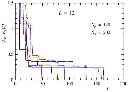
Figure 1: Lowest energy $E_{n}$ for the $n$th trial in a typical sample of the $\pm J$ Heisenberg model as a function of the generation $t$, where $E_{G}$ is a tentative ground-state energy obtained beforehand, applying the same method with a larger number of the local populations of $N_{p}=256$. Note that results for eight trials are shown, one of which (described by *) fails to get the ground-state energy because $\Delta t>100$.

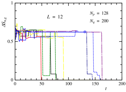
Figure 2: Distance in the spin configuration $\Delta S_{n,g}$ as a function of the generation $t$ in the same ground-state search process presented in Fig. 1.

The PfGA requires only two parameters: the number of the local populations $N_{p}$ and the number of quenching steps $N_{q}$. In contrast to the GAI, the generation number $\nu$ results from the evolution of the population. It was found that, when $N_{p}$ and $N_{q}$ are fixed, the average number $\bar{\nu}$ slowly increases with the linear size $L$, e.g., when $N_{p}=128$ and $N_{q}=100$, $\bar{\nu}$ = 154(16), 149(20), 200(20), 219(26) and 287(30), respectively, for $L$ = 8, 10, 11, 12 and 13. It was also found that, for a fixed size $L$, $\bar{\nu}$ decreases slowly as $N_{p}$ and/or $N_{q}$ increases. Although the total number of the individuals in the population S changes as the population evolves and often becomes considerably greater than $2N_{p}$, the crossover time is $2N_{p}$ at every generation. Therefore, the computer CPU time $t_{\rm II}$ is estimated as

$$t_{\rm II}=A_{\rm II}\times 2N_{p}\times\bar{\nu}\times N_{q}\times({\rm lattice\ size}\ N),$$ (5)

with $\bar{\nu}=150\sim 300$ for $L\leq 14$. The constant $A_{\rm II}$ is independent of other parameters and $A_{\rm II}\sim A_{\rm I}$. We have performed the same test in the $\pm J$ Heisenberg model; its results are presented in Table II. It is readily apparent that $t_{\rm II}/t_{\rm I}=1/4\sim 1/2$ for obtaining the ground state with the same validity; using GAII, we can extend the treatable lattice size using a personal computer from $L=12$ to $L=13$. We have calculated the ground state energy per spin, $E_{G}(L)$, for the $L\times L\times L$ ($L\leq 13$) lattice and present them in Table III. Here, the parameter set of ($N_{p},N_{q}$) has been chosen such that the search ratio becomes greater than 0.90. The numbers of samples are about 4000 for smaller lattices and about 500 for larger lattices. We have estimated the ground state energy of the model, $E_{G}(\equiv E_{G}(\infty))$, by using data for $8\leq L\leq 13$ with an extrapolation function $E_{G}(L)=E_{G}+a/L^{\lambda}$, and add it in the same table. Note that the value of $E_{G}/J=-2.0432\pm 0.0015$ is a little lower than that of $E_{G}/J\sim-2.0411$ estimated by using data for smaller lattices of $4\leq L\leq 11$[6]. Further studies are necessary to settle the value of $E_{G}$.

We have developed a new genetic algorithm (GAII) by combining the triadic crossover of the GAI and the parameter free genetic algorithm. The GAII further improves the ground-state searching efficiency. It reduces the number of parameters from four ($M_{i},\nu_{0},N_{q}$ and $\mu$ in the GAI) to two ($N_{p}$ and $N_{q}$). This is also the merit of the method because the determination of those parameters is an important but tedious task for application to different problems.

Table 2: Ratios and their standard variances of success in searching for the ground-state energy of the $\pm J$ model on $L\times L\times L$ lattice using the GAII, where $N_{p}$ and $N_{q}$ respectively denote the local population and number of quenching steps. These are estimated for 10 runs for 16 samples.

$L(N_{q})\setminus N_{p}$	16	32	64	128	256	512	1024
8 (100)	0.93(.13)	1.00(.00)	—	—	—	—	—
10 (100)	—	0.80(.18)	0.90(.14)	0.98(.03)	—	—	—
11 (100)	—	—	0.59(.20)	0.85(.17)	0.92(.13)	—	—
(200)	—	—	0.83(.14)	0.80(.17)	0.99(.03)	—	—
12 (200)	—	—	—	0.85(.17)	0.92(.12)	1.00(.00)	—
13 (400)	—	—	—	—	0.74(.22)	0.86(.20)	0.93(.13)
14 (400)	—	—	—	—	—	0.71(.19)	0.81(.23)

Table 3: The ground state energy per spin $E_{G}(L)$ of the $\pm J$ model on the $L\times L\times L$ lattice obtained by GAII. $E_{G}(\equiv E_{G}(\infty))$ is estimated by using data for $8\leq L\leq 13$.

$L$	8	10	11	12	13	$\infty$
$E_{G}(L)/J$	-2.0341(2)	-2.0376(2)	-2.0392(3)	-2.0393(3)	-2.0403(3)	-2.0432(15)

3 Stiffness of the Ground State

The most interesting ground-state property of the system is the stiffness of the model at $T=0$. The stiffness constant $\theta$ is estimated from the domain-wall (DW) energy $\Delta E_{L}$ of the $L\times L\times L$ lattice;

$$\Delta E_{L}\propto JL^{\theta},$$ (6)

for $L\rightarrow\infty$. When $\theta>0$, the SG phase transition occurs at a finite temperature, although no phase transition occurs when $\theta<0$. A mysterious problem exists, by which $\theta$ depends on the estimation method of $\Delta E_{L}$. Two methods are typically used: One is the periodic-antiperiodic (P-AP) method, in which $\theta$ is estimated as $\theta=-(0.65\sim 1.0)$[14, 15, 16]. However, this value was shown to be lattice size range dependent.[17]. The other is the open-boundary-twist (OB-Twist) method [18, 19, 20], by which one obtains $\theta=0.5\sim 1.0$ depending on the twisting manner.[17] That is, the former method predicts the absence of the phase transition at a finite temperature; the latter predicts its presence. Unfortunately, these estimations are given in small lattices of $L\leq 8$. The question is whether or not the two methods engender the same result for $L\rightarrow\infty$. Here, we reexamine $\theta$ in larger lattices using the GAII.

3.1 P-AP method

Using this method, one usually considers a simple cubic lattice of $L\times L\times L$. Here, we consider lattices with different aspect ratios $L\times L\times rL$ ($r\geq 1$) because the value of $\theta$ of the system was suggested to be properly estimated in lattices with a large ratio $r$[21, 22]. We consider the DW energy $\Delta E_{r,L}$ which is defined as the difference in the ground-state energy between the two lattices A and B with the same bond distribution but with different boundary conditions. That is, for lattice A, a periodic boundary condition is applied for every direction; for lattice B, an antiperiodic boundary condition is applied for the $z$-direction and a periodic boundary condition for the $x$- and $y$-directions. The GAII is applied to both lattices A and B to estimate the respective ground-state energies $E_{r,L}^{(A)}$ and $E_{r,L}^{(B)}$. The DW energy is calculated as [$\Delta E_{r,L}=|E_{r,L}^{(A)}-E_{r,L}^{(B)}|$], where [$\cdots$] denotes the sample average. The parameter set of ($N_{p},N_{q}$) and the numbers of the samples are the same as described in Sec. 2.2. Figure 3 shows [$\Delta E_{r,L}$] for different $r$ as functions of $L$ in a log-log form, the slope of which gives the stiffness constant $\theta$. We see that [$\Delta E_{r,L}$] for different $r$ shows different $L$ dependences; for $r=1$, it decreases with increasing $L$, but its decrement becomes smaller and seems to converge to a finite, nonzero value for $L\rightarrow\infty$; for $r=2$, it is almost independent of $L$; for $r\geq 3$, it increases with $L$ and seems to converge to a finite value. That is, the results imply that $\theta=0$, irrespective of the aspect ratio $r$. Then using an extrapolation function $[\Delta E_{r,L}]=[\Delta E_{r,\infty}]+a/L+b/L^{2}$ for $L\geq 4$, we estimate the convergence value for each of $r$: $[\Delta E_{r,\infty}]/J=0.95\pm 0.06,0.49\pm 0.06,0.36\pm 0.06$ and $0.22\pm 0.08$ for $r=1,2,3$ and 4, respectively. As expected, results fit well like in a ferromagnetic model: $[\Delta E_{r,\infty}]\propto[\Delta E_{1,\infty}]/r$. Therefore, we suggest that $\theta=0$ in the P-AP method, contrary to previous estimations of $\theta<0$.

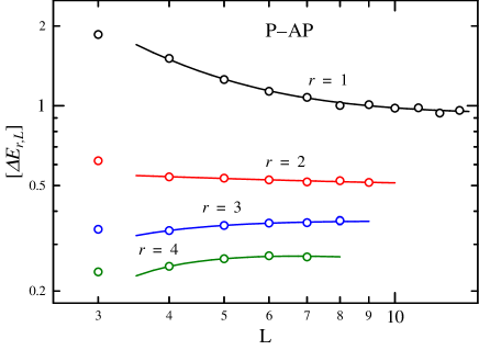
Figure 3: DW energy $\Delta E_{r,L}$ of the $L\times L\times rL$ lattice using the P-AP method. Lines are fitted ones using the function described in the text.

3.2 OB-twist method

We consider the $L\times L\times(rL+1)$ lattice with periodic boundary conditions for the $x$- and $y$-directions and the open boundary condition for the $z$-direction (the lattice has two opposite surfaces, $\Omega_{1}$ and $\Omega_{rL+1}$). We consider a twist energy, which is calculated as follows. We first determine the ground state with an energy $E_{r,L}$; then, under the condition that all the spins on $\Omega_{1}$ are fixed, all the spins on $\Omega_{rL+1}$ are twisted (rotated) at $\phi$ around the $z$-axis and the lowest energy $E_{r,L}(\phi)$ is calculated; the twist energy is given as the difference between these two energies: $\Delta E_{r,L}(\phi)=E_{r,L}(\phi)-E_{r,L}$. Using the GAII with similar conditions to those used in the P-AP method, we calculate $[\Delta E_{r,L}(\phi=\pi/2)]$ for $r=1,2,4$. The results are presented in Fig. 4 in a log-log form. In contrast to the results in the P-AP method, data for each $r$ seem to lie on a straight line, suggesting that $[\Delta E_{r,L}(\pi/2)]\propto L^{\theta}$. Their lines’ slopes are almost identical, which indicates that $\theta$ is independent of the aspect ratio $r$. Then we fit them using a stiffness constant of $\theta=0.62$, which was estimated previously in smaller lattices ($L\leq 8$) with $r=1$.[17] The quality of the results is very good, as depicted in Fig. 3. Consequently, we expect that $\theta\sim 0.62$ in the OB-twist method.

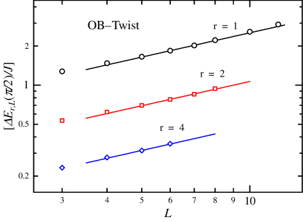
Figure 4: Twist energies $\Delta E_{r,L}(\pi/2)$ of the $L\times L\times rL$ lattice with open boundaries as functions of $L$. Lines are fitted ones using the stiffness exponent $\theta=0.62$, which was given using smaller lattices ($L\leq 8$) with $r=1$.[17]

3.3 Remarks related to the stiffness constant $\theta$

We estimated the stiffness constant $\theta$ in larger lattices using the P-AP and OB-twist methods and obtained different values, respectively, of $\theta=0$ and $\theta\sim 0.62$. That is, $\theta$ of this model depends on the estimation method, in contrast to a ferromagnetic Heisenberg model for which $\theta$ is a universal constant of $\theta=d-2$ in the $d$-dimensional system. We consider $\theta$ in those methods.

In the OB-twist method, the meaning of $\Delta E_{r,L}(\phi)$ is clear. We consider the stiffness of the ground state of the open system itself; the depth or steepness of the ground-state valley in the energy landscape of the system. In this case, the twist energy $\Delta E_{r,L}(\phi)$ is surely a lifted energy brought by a perturbation around the ground state. That is, the result for $\theta\sim 0.62$ suggests that, once the system falls into a ground-state valley at very low temperatures, it slightly escapes from the valley.

On the other hand, in the P-AP method, the calculation of $\Delta E_{r,L}$ comes from an application of the renormalization-group idea; one evaluates the effective coupling $\tilde{J}_{L}(\sim JL^{\theta})$ between block spins of the linear dimension $L$ generated by renormalization. That is, one assumes that $\tilde{J}_{L}\sim\Delta E_{r,L}$. However, the meaning of $\Delta E_{r,L}$ calculated in this method has remained unclear.[19, 20, 23] Our findings of $\theta=0$ and $[\Delta E_{r,\infty}]\propto[\Delta E_{1,\infty}]/r$ seem to reveal its meaning. We consider $\Delta E_{r,L}$ on the basis of the DW argument in the ferromagnetic Heisenberg model. The difference $\Delta E_{r,L}$ arises from the difference in the boundary condition between lattices A and B. That is, the difference in the energy between two lattices with different boundary bonds $\{J_{(i,1),(i,rL)}\}$ and $\{-J_{(i,1),(i,rL)}\}$. We first consider the open lattice with $\{J_{(i,1),(i,rL)}=0\}$ for which the ground-state spin configuration and its energy are described, respectively, as $\{\mbox{\boldmath$S$}^{0}_{i}\}$ and $E^{0}_{r,L}$. Coming back to lattice A, some boundary bonds will favor $\{\mbox{\boldmath$S$}^{0}_{i}\}$; others will obstruct it, giving the resulting energy $E^{(A)}_{r,L}$. We respectively denote the former bonds as right ($r$) -bonds and the latter bonds as wrong($w$)-bonds and their numbers as $n_{r}$ and $n_{w}$. As in the ferromagnetic case, this operation will change the energy of the lattice as $O(J/rL)$ per chain along the $z$-direction for larger $L$, $E^{(A)}_{r,L}-E^{0}_{r,L}\propto-(J/rL)\times(n_{r}-n_{w})$. In lattice B, the roles of the $r$- and $w$-bonds are reversed and $E^{(B)}_{r,L}-E^{0}_{r,L}\propto-(J/rL)\times(n_{w}-n_{r})$. Then we expect $\Delta E_{r,L}\propto JL^{\frac{d-3}{2}}/r$ for $L\gg 1$, because $|n_{r}-n_{w}|\sim L^{\frac{d-1}{2}}$ in the $d$-dimensional lattice. That is, $\theta=0$ in $d=3$ and $[\Delta E_{r,\infty}]\propto[\Delta E_{1,\infty}]/r$, as was obtained in this study. To examine the speculation, we make an additional calculation putting all the surface bonds as $r$ bonds, as in the usual DW argument in the ferromagnetic case: $\{J_{(i,1),(i,rL)}=Sign(\mbox{\boldmath$S$}^{0}_{i,1}\mbox{\boldmath$S$}^{0}_{i,rL})J\}$. We call this boundary condition an optimized boundary condition and the boundary condition with $\{-J_{(i,1),(i,rL)}\}$ an antioptimized boundary condition, and the calculation of $\Delta E_{r,L}$ in these boundary conditions as an optimized-antioptimized (Opt-AOpt) method. Results of $\Delta E_{r,L}$ for $r=1,$ and 2 are shown in Fig. 5. In fact, $\Delta E_{r,L}$ increases with $L$ for larger $L$. Interestingly, their slopes become larger with increasing $L$, implying that they reach 1 for $L\rightarrow\infty$, as suggested by the argument. Further calculations are necessary to estimate the value of $\theta$ for each $r$ and thereby its $r$-independent value. Nonetheless the Opt-AOpt method implies that $\theta>0$ in constrast with $\theta=0$ in the P-AP method. We suggest, therefore, that the $\theta$ in the P-AP method is not a universal constant that describes the effective coupling $\tilde{J}_{L}$, but a characteristic value that describes the boundary condition. It turns out the results imply that a strong correlation exists between the spin configurations on two opposite surfaces of the open lattice.

Hence, we suggest that the result of $\theta=0$ in the P-AP method and that of $\theta\sim 0.62$ in the OB-twist method indicate the same thing that the ground state of the open system is stable against a weak perturbation.

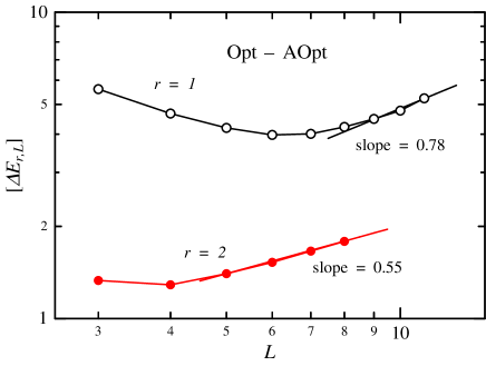
Figure 5: The DW energy $\Delta E_{r,L}$ of the $L\times L\times rL$ lattice using the Opt-AOpt method.

4 Conclusions

We developed a genetic algorithm (GA) in the Heisenberg model. We first show that the triadic crossover in the Ising model also works well in the Heisenberg model. Then, combining it with a parameter-free genetic algorithm, we proposed a useful algorithm for the Heisenberg spin-glass model.

Using the algorithm, we examined the ground-state stiffness of the $\pm J$ Heisenberg model in three dimensions. Results showed the stiffness constant of $\theta=0$ in the periodic-antiperiodic method, and that of $\theta\sim 0.62$ in the open-boundary-twist method. The origin of the difference in $\theta$ between these methods was discussed. We suggested that both results show the same thing: the open system’s ground state is stable against a weak perturbation. An interesting issue whether or not the values of the chirality stiffness constant and the spin glass stiffness constant are the same will be discussed in a separate paper.

References

- [1] A. K. Hartmann and H. Rieger: Optimization Algorithms in Physics (Wiley, Berlin, 2002).
- [2] K. F. Pál: Physica A 223 (1996) 283.
- [3] A. K. Hartmann: Phys. Rev. E 59 (1999) 84.
- [4] J. Houdayer and O.C. Martin: Phys. Rev. Lett. 83 (1999) 1030.
- [5] J. Houdayer and O.C. Martin: Phys. Rev. E 64 (1999) 056704.
- [6] F. Matsubara, T. Shirakura, S. Takahashi, and Y. Baba: Phys. Rev. B 70 (2004) 174414.
- [7] We can change this criterion of or to or , but the efficiency hardly improves.
- [8] S. Kizu, H. Sawai, and T. Endo: Proc. of the 1997 Int. Symp. on Nonlinear Theory and Its Application 2-2 (1997) 1273.
- [9] H. Sawai and S. Kizu: Proc. of the Int. Conf. on Parallel Problem Solving from Nature 1998.9 (1998) 702.
- [10] H. Sawai, S. Adachi and S. Kizu: Advances in Evolutionary Computation ed. A. Ghosh and S. Tsutsui (2003) 117, Springer Verlag.
- [11] H. Bersini et al.: 1996 IEEE Int. Conf. on Evolutionary Computation (ICEO’96) (1996) 611.
- [12] M. Furusawa and H. Doi: J. Theor. Biol. 157 (1992) 127.
- [13] K. Wada, H. Doi, S. Tanaka, Y. Wada, and M. Furusawa: Proc. Natl. Acad. Sci., USA 90 (1993) 11934.
- [14] J. R. Banavar and M. Cieplak: Phys. Rev. Lett. 48 (1982) 832.
- [15] W. L. McMillan: Phys. Rev. B 31 (1984) 342.
- [16] H. Kawamura: Phys. Rev. Lett. 68 (1992) 3785.
- [17] F. Matsubara, T. Shirakura, S. Endo, and S. Takahashi: J. Phys. A: Math. Gen. 36 (2003) 10881.
- [18] F. Matsubara, T. Shirakura, and M. Shiomi: Phys. Rev. B 58 (1998) R11821.
- [19] F. Matsubara, S. Endoh, and T. Shirakura: J. Phys. Soc. Jpn. 69 (2000) 1927.
- [20] S. Endoh, F. Matsubara, and T. Shirakura: J. Phys. Soc. Jpn. 70 (2001) 1543.
- [21] A. C. Carter, A. J. Bray, and M. A. Moore: Phys. Rev. Lett. 88 (2002) 077201.
- [22] M. Weigel and M. J. P. Gingras: Phys. Rev. Lett. 96 (2006) 097206.
- [23] J. M. Kosterlitz and N. Akino: Phys. Rev. Lett. 82 (1999) 4094.