Recent Progress on Tau Lepton Physics

Abstract

Some important aspects of hadronic $\tau$ decays are reviewed: the determination of $\alpha_{s}$ from the inclusive $\tau$ hadronic width, the measurement of $|V_{us}|$ through the Cabibbo-suppressed decays of the $\tau$, and the theoretical description of the $\tau\to\nu_{\tau}K\pi$ spectrum. The present status of other relevant electroweak topics, such as charged-current universality tests or bounds on lepton-flavour violation, has been already summarized in ref. [1].

1 The inclusive hadronic width of the tau

The hadronic $\tau$ decays turn out to be a beautiful laboratory for studying strong interaction effects at low energies [2, 3]. The $\tau$ is the only known lepton massive enough to decay into hadrons. Its semileptonic decays are then ideally suited for studying the hadronic weak currents.

The inclusive character of the total $\tau$ hadronic width renders possible an accurate calculation of the ratio [4, 5, 6, 7, 8]

$$R_{\tau}\equiv{\Gamma[\tau^{-}\to\nu_{\tau}\,\mathrm{hadrons}]\over\Gamma[\tau^{-}\to\nu_{\tau}e^{-}{\bar{\nu}}_{e}]}\,=\,R_{\tau,V}+R_{\tau,A}+R_{\tau,S}\,.$$

The theoretical analysis involves the two-point correlation functions for the vector $\,V^{\mu}_{ij}=\bar{\psi}_{j}\gamma^{\mu}\psi_{i}\,$ and axial-vector $\,A^{\mu}_{ij}=\bar{\psi}_{j}\gamma^{\mu}\gamma_{5}\psi_{i}\,$ colour-singlet quark currents ($i,j=u,d,s$):

$$\Pi^{\mu\nu}_{ij,{\cal J}}(q)\equiv i\int d^{4}x\,e^{iqx}\langle 0|T({\cal J}^{\mu}_{ij}(x){\cal J}^{\nu}_{ij}(0)^{\dagger})|0\rangle,$$ (1)

which have the Lorentz decompositions

$$\Pi^{\mu\nu}_{ij,{\cal J}}(q) \!\!\!\!= \!\!\!\!(-g^{\mu\nu}q^{2}+q^{\mu}q^{\nu})\,\Pi_{ij,{\cal J}}^{(1)}(q^{2})$$ (2)

$$\!\!\!\!+q^{\mu}q^{\nu}\,\Pi_{ij,{\cal J}}^{(0)}(q^{2}),$$

where the superscript $(J=0,1)$ denotes the angular momentum in the hadronic rest frame.

The imaginary parts of $\,\Pi^{(J)}_{ij,{\cal J}}(q^{2})\,$ are proportional to the spectral functions for hadrons with the corresponding quantum numbers. The semihadronic decay rate of the $\tau$ can be written as an integral of these spectral functions over the invariant mass $s$ of the final-state hadrons:

$$R_{\tau} \!\!\!\!\!= \!\!\!\!\!12\pi\int^{m_{\tau}^{2}}_{0}{ds\over m_{\tau}^{2}}\,\left(1-{s\over m_{\tau}^{2}}\right)^{2}$$ (3)

$$\!\!\!\!\!\times \!\!\!\!\!\biggl{[}\left(1+2{s\over m_{\tau}^{2}}\right)\mbox{\rm Im}\Pi^{(1)}(s)+\mbox{\rm Im}\Pi^{(0)}(s)\biggr{]}.$$

The appropriate combinations of correlators are

$$\Pi^{(J)}(s) \!\!\!\equiv \!\!\!|V_{ud}|^{2}\,\left(\Pi^{(J)}_{ud,V}(s)+\Pi^{(J)}_{ud,A}(s)\right)$$ (4)

$$\!\!\!+ \!\!\!|V_{us}|^{2}\,\left(\Pi^{(J)}_{us,V}(s)+\Pi^{(J)}_{us,A}(s)\right).$$

The contributions coming from the first two terms correspond to $R_{\tau,V}$ and $R_{\tau,A}$ respectively, while $R_{\tau,S}$ contains the remaining Cabibbo-suppressed contributions.

The integrand in Eq. (3) cannot be calculated at present from QCD. Nevertheless the integral itself can be calculated systematically by exploiting the analytic properties of the correlators $\Pi^{(J)}(s)$. They are analytic functions of $s$ except along the positive real $s$-axis, where their imaginary parts have discontinuities. $R_{\tau}$ can then be written as a contour integral in the complex $s$-plane running counter-clockwise around the circle $|s|=m_{\tau}^{2}$:

$$R_{\tau} \!\!\!\!\!= \!\!\!\!\!6\pi i\oint_{|s|=m_{\tau}^{2}}{ds\over m_{\tau}^{2}}\,\left(1-{s\over m_{\tau}^{2}}\right)^{2}$$ (5)

$$\!\!\!\!\!\times \!\!\!\!\!\left[\left(1+2{s\over m_{\tau}^{2}}\right)\Pi^{(0+1)}(s)-2{s\over m_{\tau}^{2}}\Pi^{(0)}(s)\right]\!.$$

This expression requires the correlators only for complex $s$ of order $m_{\tau}^{2}$, which is significantly larger than the scale associated with non-perturbative effects. Using the Operator Product Expansion (OPE), $\Pi^{(J)}(s)=\sum_{D}C_{D}^{(J)}/(-s)^{D/2}$, to evaluate the contour integral, $R_{\tau}$ can be expressed as an expansion in powers of $1/m_{\tau}^{2}$. The uncertainties associated with the use of the OPE near the time-like axis are heavily suppressed by the presence in (5) of a double zero at $s=m_{\tau}^{2}$.

The combination $R_{\tau,V+A}$ can be written as [6]

$$R_{\tau,V+A}\,=\,N_{C}\,|V_{ud}|^{2}\,S_{\mathrm{EW}}\left\{1+\delta_{\mathrm{P}}+\delta_{\mathrm{NP}}\right\},$$ (6)

where $N_{C}=3$ is the number of quark colours and $S_{\mathrm{EW}}=1.0201\pm 0.0003$ contains the electroweak radiative corrections [9, 10, 11]. The dominant correction ($\sim 20\%$) is the perturbative QCD contribution $\delta_{\mathrm{P}}$, which is already known to $O(\alpha_{s}^{4})$ [6, 12] and includes a resummation of the most important higher-order effects [7, 13].

Non-perturbative contributions are suppressed by six powers of the $\tau$ mass [6] and, therefore, are very small. Their numerical size has been determined from the invariant-mass distribution of the final hadrons in $\tau$ decay, through the study of weighted integrals [14],

$$R_{\tau}^{kl}\,\equiv\,\int_{0}^{m_{\tau}^{2}}ds\,\left(1-{s\over m_{\tau}^{2}}\right)^{k}\,\left({s\over m_{\tau}^{2}}\right)^{l}\,{dR_{\tau}\over ds}\,,$$ (7)

which can be calculated theoretically in the same way as $R_{\tau}$. The predicted suppression [6] of the non-perturbative corrections has been confirmed by ALEPH [15], CLEO [16] and OPAL [17]. The most recent analysis [18] gives

$$\delta_{\mathrm{NP}}\,=\,-0.0059\pm 0.0014\,.$$ (8)

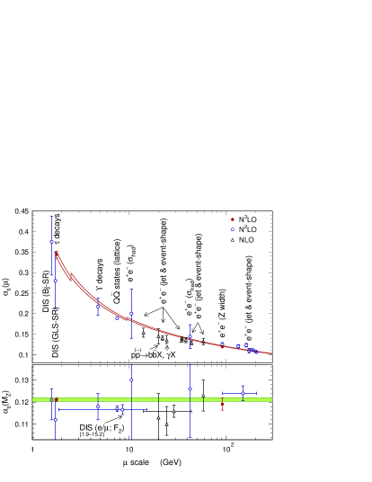
Figure 1: Measured values of $\alpha_{s}$ at different scales. The curves show the energy dependence predicted by QCD, using $\alpha_{s}(m_{\tau}^{2})$ as input. The corresponding extrapolated $\alpha_{s}(M_{Z}^{2})$ values are shown at the bottom, where the shaded band displays the $\tau$ decay result within errors [18].

The QCD prediction for $R_{\tau,V+A}$ is then completely dominated by $\delta_{P}$; non-perturbative effects being smaller than the perturbative uncertainties from uncalculated higher-order corrections. The result turns out to be very sensitive to the value of $\alpha_{s}(m_{\tau}^{2})$, allowing for an accurate determination of the fundamental QCD coupling [5, 6]. The experimental measurement $R_{\tau,V+A}=3.479\pm 0.011$ implies [18]

$$\alpha_{s}(m_{\tau}^{2})\,=\,0.344\pm 0.005_{\mathrm{exp}}\pm 0.007_{\mathrm{th}}\,.$$ (9)

The strong coupling measured at the $\tau$ mass scale is significantly larger than the values obtained at higher energies. From the hadronic decays of the $Z$, one gets $\alpha_{s}(M_{Z}^{2})=0.1191\pm 0.0027$ [12, 18, 19], which differs from $\alpha_{s}(m_{\tau}^{2})$ by more than $20\,\sigma$. After evolution up to the scale $M_{Z}$ [20], the strong coupling constant in (9) decreases to [18]

$$\alpha_{s}(M_{Z}^{2})\,=\,0.1212\pm 0.0011\,,$$ (10)

in excellent agreement with the direct measurements at the $Z$ peak and with a better accuracy. The comparison of these two determinations of $\alpha_{s}$ in two very different energy regimes, $m_{\tau}$ and $M_{Z}$, provides a beautiful test of the predicted running of the QCD coupling; i.e., a very significant experimental verification of asymptotic freedom.

2 Perturbative contribution to $R_{\tau}$

The recent calculation of the ${\cal O}(\alpha_{s}^{4})$ contribution to $\Pi^{(0+1)}(s)$ [12] has triggered a renewed theoretical interest on $R_{\tau}$ [12, 18, 21, 22]. The perturbative contribution $\delta_{P}$ is extracted from the Adler function

$$-s{d\over ds}\Pi^{(0+1)}(s)={1\over 4\pi^{2}}\sum_{n=0}K_{n}\left({\alpha_{s}(s)\over\pi}\right)^{n}.$$ (11)

For three flavours, the known coefficients take the values: $K_{0}=K_{1}=1$; $K_{2}=1.63982$; $K_{3}(\overline{MS})=6.37101$ and $K_{4}(\overline{MS})=49.07570$ [12].

The perturbative component of $R_{\tau}$ is given by

$$\delta_{P}=\sum_{n=1}K_{n}\,A^{(n)}(\alpha_{s}),$$ (12)

where the functions [7]

$$A^{(n)}(\alpha_{s}) \!\!\!\!= \!\!\!\!{1\over 2\pi i}\oint_{|s|=m_{\tau}^{2}}{ds\over s}\,\left({\alpha_{s}(-s)\over\pi}\right)^{n}$$ (13)

$$\!\!\!\!\times \!\!\!\!\left(1-2{s\over m_{\tau}^{2}}+2{s^{3}\over m_{\tau}^{6}}-{s^{4}\over m_{\tau}^{8}}\right)$$

are contour integrals in the complex plane, which only depend on $a_{\tau}\equiv\alpha_{s}(m_{\tau}^{2})/\pi$. Using the exact solution (up to unknown $\beta_{n>4}$ contributions) for $\alpha_{s}(s)$ given by the renormalization-group $\beta$-function equation, they can be numerically computed with a very high accuracy [7]. One can easily check that the results are very stable under changes of the renormalization scale and rather insensitive to the truncation of the $\beta$ function (putting $\beta_{4}=0$ has a negligible impact). Thus, the resulting theoretical uncertainty on $\delta_{P}$ is small.

However if, instead of adopting the known values for $A^{(n)}(\alpha_{s})$, one expands $\alpha_{s}(-s)$ in powers of $\alpha_{s}(m_{\tau})$ inside the the integrals (13), the large logarithmic running along the circle $s=m_{\tau}^{2}\exp{(i\phi)}$ ($\phi\epsilon[0,2\pi]$) gives rise to a nearly divergent series of the form $\delta_{P}\,=\,\sum_{n=1}(K_{n}+g_{n})\,a_{\tau}^{n}$, where the $g_{n}$ coefficients depend on $K_{m<n}$ and on $\beta_{m<n}$:

$$\delta^{(0)}=a_{\tau}+5.20\,a_{\tau}^{2}+26.4\,a_{\tau}^{3}+127\,a_{\tau}^{4}+\,\cdots$$ (14)

The “running” $g_{n}$ contributions are much larger than the original $K_{n}$ coefficients containing the Adler function dynamics ($g_{2}=3.563$, $g_{3}=19.99$, $g_{4}=78.00$) [7]. These generates a sizeable renormalization scale dependence, which is much larger than the naively expected ${\cal O}(\alpha_{s}^{5})$ effect. The radius of convergence of this expansion is actually quite small. A numerical analysis of the series [7] shows that, at the three-loop level, an upper estimate for the convergence radius is $a_{\tau,\mbox{\rm\scriptsize conv}}\,<0.11$, which is very close to the physical value. Thus, the fixed-order expansion (14) should not be used for accurate predictions of $R_{\tau}$. The result (9) has been correctly obtained using Eq. (12) with the exact values of the functions $A^{(n)}(\alpha_{s})$. The slightly different results quoted in refs. [12, 21] originate in their use of the pathological fixed-order expansion (14).

3 $|V_{us}|$ determination from tau decays

The separate measurement of the $|\Delta S|=0$ and $|\Delta S|=1$ tau decay widths provides a very clean determination of $V_{us}\,$ [23, 24]. To a first approximation the Cabibbo mixing can be directly obtained from experimental measurements, without any theoretical input. Neglecting the small SU(3)-breaking corrections from the $m_{s}-m_{d}$ quark-mass difference, one gets:

$$|V_{us}|^{\mathrm{SU(3)}}=\>|V_{ud}|\>\left(\frac{R_{\tau,S}}{R_{\tau,V+A}}\right)^{1/2}=\>0.210\pm 0.003\,.$$

We have used $|V_{ud}|=0.97418\pm 0.00027$ [25], $R_{\tau}=3.640\pm 0.010$ and the value $R_{\tau,S}=0.1617\pm 0.0040$ [24], which results from the most recent BaBar [26] and Belle [27] measurements of Cabibbo-suppressed tau decays [28]. The new branching ratios measured by BaBar and Belle are all smaller than the previous world averages, which translates into a smaller value of $R_{\tau,S}$ and $|V_{us}|$. For comparison, the previous value $R_{\tau,S}=0.1686\pm 0.0047$ [18] resulted in $|V_{us}|^{\mathrm{SU(3)}}=0.215\pm 0.003$.

This rather remarkable determination is only slightly shifted by the small SU(3)-breaking contributions induced by the strange quark mass. These corrections can be estimated through a QCD analysis of the differences [23, 24, 29, 30, 31, 32, 33, 34, 35, 36]

$$\delta R_{\tau}^{kl}\,\equiv\,{R_{\tau,V+A}^{kl}\over|V_{ud}|^{2}}-{R_{\tau,S}^{kl}\over|V_{us}|^{2}}\,.$$ (15)

The only non-zero contributions are proportional to the mass-squared difference $m_{s}^{2}-m_{d}^{2}$ or to vacuum expectation values of SU(3)-breaking operators such as $\delta O_{4}\equiv\langle 0|m_{s}\bar{s}s-m_{d}\bar{d}d|0\rangle\approx(-1.4\pm 0.4)\cdot 10^{-3}\;\mathrm{GeV}^{4}$ [29, 23]. The dimensions of these operators are compensated by corresponding powers of $m_{\tau}^{2}$, which implies a strong suppression of $\delta R_{\tau}^{kl}$ [29]:

$$\delta R_{\tau}^{kl} \!\!\approx \!\!24\,S_{\mathrm{EW}}\;\left\{{m_{s}^{2}(m_{\tau}^{2})\over m_{\tau}^{2}}\,\left(1-\epsilon_{d}^{2}\right)\,\Delta_{kl}(\alpha_{s})\right.$$ (16)

$$\hskip 36.98866pt\left.-2\pi^{2}\,{\delta O_{4}\over m_{\tau}^{4}}\,Q_{kl}(\alpha_{s})\right\}\,,$$

where $\epsilon_{d}\equiv m_{d}/m_{s}=0.053\pm 0.002$ [37]. The perturbative corrections $\Delta_{kl}(\alpha_{s})$ and $Q_{kl}(\alpha_{s})$ are known to $O(\alpha_{s}^{3})$ and $O(\alpha_{s}^{2})$, respectively [29, 36].

The $J=0$ contribution to $\Delta_{00}(\alpha_{s})$ shows a rather pathological behaviour, with clear signs of being a non-convergent perturbative series. Fortunately, the corresponding longitudinal contribution to $\delta R_{\tau}\equiv\delta R_{\tau}^{00}$ can be estimated phenomenologically with a much better accuracy, $\delta R_{\tau}|^{L}\,=\,0.1544\pm 0.0037$ [23, 38], because it is dominated by far by the well-known $\tau\to\nu_{\tau}\pi$ and $\tau\to\nu_{\tau}K$ contributions. To estimate the remaining transverse component, one needs an input value for the strange quark mass. Taking the range $m_{s}(m_{\tau})=(100\pm 10)\>\mathrm{MeV}$  [$m_{s}(2\>\mathrm{GeV})=(96\pm 10)\>\mathrm{MeV}$], which includes the most recent determinations of $m_{s}$ from QCD sum rules and lattice QCD [38], one gets finally $\delta R_{\tau,th}=0.216\pm 0.016$, which implies [24]

$$|V_{us}| = \left(\frac{R_{\tau,S}}{\frac{R_{\tau,V+A}}{|V_{ud}|^{2}}-\delta R_{\tau,\mathrm{th}}}\right)^{1/2}$$ (17)

$$= 0.2165\pm 0.0026_{\mathrm{\,exp}}\pm 0.0005_{\mathrm{\,th}}\,.$$

A larger central value, $|V_{us}|=0.2212\pm 0.0031$, is obtained with the old world average for $R_{\tau,S}$.

Sizeable changes on the experimental determination of $R_{\tau,S}$ are to be expected from the full analysis of the huge BaBar and Belle data samples. In particular, the high-multiplicity decay modes are not well known at present. Thus, the result (17) could easily fluctuate in the near future. However, it is important to realize that the final error of the $V_{us}$ determination from $\tau$ decay is completely dominated by the experimental uncertainties. If $R_{\tau,S}$ is measured with a 1% precision, the resulting $V_{us}$ uncertainty will get reduced to around 0.6%, i.e. $\pm 0.0013$, making $\tau$ decay the best source of information about $V_{us}$.

An accurate measurement of the invariant-mass distribution of the final hadrons could make possible a simultaneous determination of $V_{us}$ and the strange quark mass, through a correlated analysis of several weighted differences $\delta R_{\tau}^{kl}$. The extraction of $m_{s}$ suffers from theoretical uncertainties related to the convergence of the perturbative series $\Delta_{kl}(\alpha_{s})$, which makes necessary a better understanding of these corrections.

4 $\tau\to\nu_{\tau}K\pi$ and $K\to\pi l\bar{\nu}_{l}$

The decays $\tau\to\nu_{\tau}K\pi$ probe the same hadronic form factors investigated in $K_{l3}$ processes, but they are sensitive to a much broader range of invariant masses. A theoretical understanding of the form factors can be achieved, using analyticity, unitarity and some general properties of QCD, such as chiral symmetry and the short-distance asymptotic behaviour [2, 3].

Figure 2 compares the resulting theoretical description of the $\tau$ decay spectrum [39] with the recent Belle measurement [27]. At low values of $s$ there is clear evidence of the scalar contribution, which was predicted previously using a careful analysis of $K\pi$ scattering data [38, 40]. From the measured $\tau$ spectrum one obtains $M_{K^{*}}=895.3\pm 0.2$ MeV and $\Gamma_{K^{*}}=47.5\pm 0.4$ MeV [39]. Since the absolute normalization is fixed by $K_{l3}$ data to be $|V_{us}|\,f_{+}^{K^{0}\pi^{-}}(0)=0.21664\pm 0.00048$ [41], one gets then a theoretical prediction for the branching fraction, Br$(\tau^{-}\to\nu_{\tau}K_{S}\pi^{-})=0.427\pm 0.024\%$, in good agreement with the Belle measurement $0.404\pm 0.013\%$, although slightly larger.

The $\tau$ determination of the vector form factor $f_{+}^{K\pi}(s)$ [39, 42] provides precise values for its slope and curvature, $\lambda_{+}^{\prime}=(25.2\pm 0.3)\cdot 10^{-3}$ and $\lambda_{+}^{\prime\prime}=(12.9\pm 0.3)\cdot 10^{-4}$ [39], in agreement but more precise than the corresponding $K_{l3}$ measurements [41].

Figure 2: Theoretical description [39] (solid line) of the Belle $\tau^{-}\to\nu_{\tau}K_{S}\pi^{-}$ data [27]. The $K^{*^{\prime}}$ (dashed-dotted) and scalar (dotted) contributions are also shown.

References

- [1] A. Pich, Nucl. Phys. B (Proc. Suppl.) 181-182 (2008) 300; 169 (2007) 393.
- [2] A. Pich, Int. J. Mod. Phys. A 21 (2006) 5652.
- [3] A. Pich, Tau Physics, in Heavy Flavours II, eds. A.J. Buras and M. Lindner, Advanced Series on Directions in High Energy Physics 15 (World Scientific, Singapore, 1998) p. 453, arXiv:hep-ph/9704453.
- [4] E. Braaten, Phys. Rev. Lett. 60 (1988) 1606; Phys. Rev. D 39 (1989) 1458.
- [5] S. Narison and A. Pich, Phys. Lett. B 211 (1988) 183.
- [6] E. Braaten, S. Narison and A. Pich, Nucl. Phys. B 373 (1992) 581.
- [7] F. Le Diberder and A. Pich, Phys. Lett. B 286 (1992) 147.
- [8] A. Pich, Nucl. Phys. B (Proc. Suppl.) 39B,C (1995) 326.
- [9] W.J. Marciano and A. Sirlin, Phys. Rev. Lett. 61 (1988) 1815.
- [10] E. Braaten and C.S. Li, Phys. Rev. D 42 (1990) 3888.
- [11] J. Erler, Rev. Mex. Phys. 50 (2004) 200.
- [12] P.A. Baikov, K.G. Chetyrkin and J.H. Kühn, Phys. Rev. Lett. 101 (2008) 012002.
- [13] A.A. Pivovarov, Z. Phys. C 53 (1992) 461.
- [14] F. Le Diberder and A. Pich, Phys. Lett. B 289 (1992) 165.
- [15] ALEPH Collaboration, Phys. Rep. 421 (2005) 191; Eur. Phys. J. C 4 (1998) 409; Phys. Lett. B 307 (1993) 209.
- [16] CLEO Collaboration, Phys. Lett. B 356 (1995) 580.
- [17] OPAL Collaboration, Eur. Phys. J. C 7 (1999) 571.
- [18] M. Davier et al., Rev. Mod. Phys. 78 (2006) 1043; Eur. Phys. J. C 56 (2008) 305.
-
[19]
The LEP Collaborations ALEPH, DELPHI, L3 and OPAL and the LEP
Electroweak Working Group, arXiv:0712.0929 [hep-ex];
http://www.cern.ch/LEPEWWG/. - [20] G. Rodrigo, A. Pich and A. Santamaria, Phys. Lett. B 424 (1998) 367.
- [21] M. Beneke and M. Jamin, JHEP 0809 (2008) 044.
- [22] K. Maltman and T. Yavin, arXiv:0807.0650 [hep-ph].
- [23] E. Gámiz et al., Phys. Rev. Lett. 94 (2005) 011803; JHEP 0301 (2003) 060.
- [24] E. Gámiz et al., PoS KAON 008 (2007).
- [25] C. Amsler et al., The Review of Particle Physics, Phys. Lett. B 667, 1 (2008).
- [26] BaBar Collaboration, Phys. Rev. Lett. 100 (2008) 011801; Phys. Rev. D 76 (2007) 051104.
- [27] Belle Collaboration, Phys. Lett. B 654 (2007) 65; 643 (2006) 5.
- [28] S. Banerjee, PoS KAON 009 (2007).
- [29] A. Pich and J. Prades, JHEP 9910 (1999) 004; 9806 (1998) 013.
- [30] S. Chen et al., Eur. Phys. J. C 22 (2001) 31. M. Davier et al., Nucl. Phys. B (Proc. Suppl.) 98 (2001) 319.
- [31] K.G. Chetyrkin, J.H. Kühn and A.A. Pivovarov, Nucl. Phys. B 533 (1998) 473.
- [32] J.G. Körner, F. Krajewski and A.A. Pivovarov, Eur. Phys. J. C 20 (2001) 259.
- [33] K. Maltman and C.E. Wolfe, Phys. Lett. B 639 (2006) 283. K. Maltman et al. arXiV:0807.3195 [hep-ph].
- [34] J. Kambor and K. Maltman, Phys. Rev. D 62 (2000) 093023; 64 (2001) 093014.
- [35] K. Maltman, Phys. Rev. D 58 (1998) 093015.
- [36] P.A. Baikov, K.G. Chetyrkin and J.H. Kühn, Phys. Rev. Lett. 95 (2005) 012003.
- [37] H. Leutwyler, Phys. Lett. B 378 (1996) 313.
- [38] M. Jamin, J.A. Oller and A. Pich, Phys. Rev. D 74 (2006) 074009.
- [39] M. Jamin, A. Pich and J. Portolés, Phys. Lett. B 640 (2006) 176; 664 (2008) 78.
- [40] M. Jamin, J.A. Oller, and A. Pich, Nucl. Phys. B 587 (2000) 331; 622 (2002) 279; Eur. Phys. J. C 24 (2002) 237.
- [41] FlaviaNet Working Group on Kaon Decays, Nucl. Phys. B (Proc. Suppl.) 181–182 (2008) 83.
- [42] D.R. Boito et al. arXiv:0807.4883 [hep-ph].