Nonlocal-local multimode bifurcation in turbulence

Abstract

It is shown that a mechanism of energy redistribution and dissipation by the inertial waves can be effectively utilized in isotropic turbulence at small Reynolds numbers. This mechanism totally suppresses the local interactions (cascades) in isotropic turbulence at the Taylor-scale based Reynolds number $R_{\lambda}<10^{2}$. This value of $R_{\lambda}$ (that can be considered as a bifurcation value at which the local regime emerges from the nonlocal one in isotropic turbulence) is in agreement with recent direct numerical simulations data. Applicability of this approach to channel flows is also briefly discussed. A theory of multimode bifurcations has been developed in order to explain anomalous (in comparison with the Landau-Hopf bifurcations) properties of the nonlocal-local bifurcation in isotropic turbulence.

I Introduction

Thanks to increase of resolution of direct numerical simulations (DNS) the significant problem of emergence of the local interactions in isotropic turbulence became available for a quantitative investigation (see, for instance, Refs. gfn -map and references therein). Using the DNS data it is shown in a recent paper b1 that nonlocal interactions are completely dominating in low Reynolds number isotropic turbulence, as well as in a near dissipation range at moderate and large Reynolds numbers. The bottleneck phenomenon f ,lm , produced by these interactions, has an universal character. In corresponding near-dissipation range of scales b1 : $\eta<r<\eta_{s}$ the nonlocal interactions are completely dominating ones in isotropic turbulence (where $\eta_{s}\simeq 27\eta$ and $\eta$ is the dissipation or Kolmogorov scale). Another scale: $r_{c}$, is a ’stability exchange”’ scale b2 . Namely, for scales $r>r_{c}$, the local (cascade) regime is stable and the nonlocal regime is unstable, whereas for scales $r<r_{c}$ the local regime is unstable and the nonlocal regime is stable. The normalized scale $\eta_{s}/\eta$ is constant b1 whereas $r_{c}/\eta$ increases with $R_{\lambda}$ b2 . Therefore, there is a value of $R_{\lambda}$ at which $r_{c}=\eta_{s}$ (see Figs. 1 and 2). This value of $R_{\lambda}$ can be considered as a bifurcation value of Reynolds number at which the local regime (still unstable) emerges from the nonlocal one. In present paper a phenomenological approach is suggested in order to compute bifurcation value of $R_{\lambda}$.

There is an overlapping of the local and nonlocal regimes in the range of scales $r_{c}>r>\eta_{s}$ b1 ,b2 . Moreover, in the turbulent environment even the bifurcation scale $\eta_{s}$ might fluctuate around its mean-field value along with the dissipation scale $\eta$ (see ssy ,b1 ,biferale ). Hence, at the nonlocal-local bifurcation the supercritical and subcritical secondary oscillations should co-exist. However, at the Landau-Hopf bifurcation this cannot be possible (see, for instance, Refs. ll ,gh ). In order to explain this ’anomalous’ behavior of the nonlocal-local bifurcation we will develop a theory of multimode bifurcations. In this theory several modes (which frequencies are in certain specific relationships) are exited simultaneously. At a bifurcation in a turbulent environment at least second harmonic should be taken into account. From dynamical point of view this situation is more complex than the one-mode (Landau-Hopf) bifurcation and corresponding dynamical equations for the exited modes are multidimensional (in the one-mode Landau-Hopf bifurcation the dynamical equation for the exited mode is two-dimensional in real variables). It is well known that behavior of dynamical systems with dimension more than two is significantly different from the two-dimensional dynamical systems. In particular, the former equations can generate stochastic attractors. This gives to the multimodal bifurcations considerable capacity in the phase space, which (unlike to the one-mode bifurcations) provide the multimode bifurcations a possibility to survive in turbulent environment.

II Phenomenology

A large vortex produces a Coriolis force field in the domain of space that it occupies, which is due to the rotational motion of the vortex. The comparatively slow motion of a large vortex affords time for the process of radiation of inertial waves to be realized by small-scale fluctuations in the Coriolis force field of this vortex it ,hgm . Such inertial waves transfer the energy being emitted by the fluctuations to the viscous layers on solid walls or to the viscous layers generated by the inertial waves on the effective boundaries of the large scale vortices phi . It is known that the energy brought by the inertial waves to the viscous layers dissipates effectively therein it ,hgm ,phi . The dissipation layer of inertial waves has a thickness of order

$$l\propto(\nu/\Omega)^{1/2},$$

where $~{}\nu~{}$ is the molecular viscosity, and $~{}\Omega~{}$ is a characteristic angular velocity of the large-scale vortex. To estimate the value of $~{}\Omega,~{}$ one can use $\Omega\propto 2\pi u_{0}/L.$ where $u_{0}$ is a typical large-scale velocity, and $L$ is a typical scale of the large-scale vortices. Then

$$l\propto(\nu~{}L/2\pi u_{0})^{1/2}.$$

If we define large-scale Reynolds number $R_{L}=Lu_{0}/\nu$, then we obtain

$$l\propto\frac{L}{\sqrt{2\pi}R_{L}^{1/2}}.$$

Or, using the Taylor-scale based Reynolds number $R_{\lambda}\simeq 4(R_{L})^{1/2}$ hin ,l ,

$$l\propto\frac{4L}{\sqrt{2\pi}R_{\lambda}}$$

The dissipative layer of the inertial waves is the ’friction’ layer of the corresponding large-scale vortices.

Part of the energy entrained by the inertial waves dissipates in the viscous layers while another part, being reflected, returns to the volume occupied by the bulk of the vortex. Decay of turbulent fluctuation kinetic energy a result of its removal by inertial waves to the ’friction’ layers can be described by equation it :

$$\frac{d\langle u^{2}\rangle}{dt}=-\alpha\frac{(\nu\Omega)^{1/2}}{L}~{}\langle u^{2}\rangle,$$

where  $\alpha~{}$ is a dimensionless constant. If $~{}\Omega~{}$ and $~{}L~{}$ are considered constants (or slowly changing), then it follows from (5):

$$\langle u^{2}\rangle\propto exp-\lambda t,$$

where $~{}\lambda=\alpha(\nu\Omega)^{1/2}/L~{}$. This decay can be taken into account in the equation for the spectral tensor in the ”external friction” approximation it :

$$\frac{\partial E_{ij}}{\partial t}=T_{ij}(k,t)-\lambda E_{ij},$$

where $~{}T_{ij}~{}$ characterizes the spectral energy transfer due to the nonlinear effects. The ”external friction” reflects the interaction between inertial effects and the viscous (’friction’) layers, and it is a phenomenological substitute to the viscous term. Since the inertial term in the Navier-Stokes equation is quadratic in the velocity, then for small $~{}E_{ij}~{}$ the functional $~{}T_{ij}~{}$ is a homogeneous functional of $~{}E_{ij}~{}$ of order 3/2. Let us make the substitution

$$E_{ij}^{*}(k,t)=E_{ij}(k,t)e^{-\lambda t}.$$

Substituting (8) into (7) we obtain

$$\frac{\partial E_{ij}^{*}}{\partial t}=T_{ij}(k,t)~{}e^{-\lambda t/2}.$$

Now, we make a replacement of the time

$$t^{{}^{\prime}}=\frac{2}{\lambda}(1-e^{-\lambda t/2}).$$

Then it follows from (9) that

$$\frac{\partial E_{ij}^{*}}{\partial t^{{}^{\prime}}}=T_{ij}(k,t^{{}^{\prime}}).$$

Replacements (8) and (10) reduce the problem with ”external friction” to a problem without friction (the initial conditions are evidently identical). As $t\rightarrow\infty~{}$, it follows from (10) that $~{}t^{{}^{\prime}}\rightarrow 2/\lambda,~{}$ so that the whole evolution with ”external friction”, Eq. (7), is stacked in the interval $~{}(0,~{}2/\lambda)~{}$ of the evolution described by ideal Eq. (11).

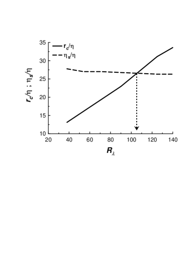
Figure 1: Scales $r_{c}/\eta$ (solid line) b2 and $\eta_{s}/\eta$ b1 (dashed line) vs. $R_{\lambda}$. The arrow indicates the transitional value of the $R_{\lambda}\simeq 10^{2}$.

On the other hand, it is known (see, for instance, Refs. es ,pg ,pelz ) that there is a certain characteristic time of an inviscid cascade process development

$$t_{c}\simeq 2~{}\frac{L}{u_{0}}$$

Taking the preceding into account, an estimate can be made of the condition under which the cascade process cannot be developed successfully (because of the action of the ”external friction”). This condition has the form

$$2/\lambda~{}<t_{c}\simeq 2~{}\frac{L}{u_{0}},$$

or

$$2L/\alpha(\nu\Omega)^{1/2}~{}<~{}2~{}\frac{L}{u_{0}}.$$

Using estimate $~{}\alpha\simeq 10~{}$ it we can rewrite condition (14) in the form

$$R_{\lambda}<10^{2}.$$

Thus, in isotropic turbulence with $R_{\lambda}<10^{2}$ the cascade process (local interactions) cannot be developed successfully (cf. Ref. demo ). Figure 1 shows dependence of the scales $r_{c}/\eta$ b2 and $\eta_{s}/\eta$ b1 on $R_{\lambda}$. Intersection of the lines: $r_{c}/\eta$ vs. $R_{\lambda}$ and $\eta_{s}/\eta$ vs. $R_{\lambda}$, indicates the transitional value of $R_{\lambda}\simeq 10^{2}$ (see Eq. (15) and Introduction). Figure 2 illustrates the transition as it appears in the energy spectra of isotropic turbulence.

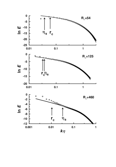
Figure 2: Three-dimensional spectra from a DNS performed in gfn for different Reynolds numbers. The solid curves in this figure correspond to the best fit by nonlocal interactions b1 .

III Separation

One can also try to apply the above consideration to channel flows. The large-scale vortices acquire a metastable state in channel turbulence because of the action of inertial forces. These forces are equilibrated by viscous friction on the solid walls of the motion domain. The dissipative layer of the inertial waves on the solid walls is the ’friction’ layer of the corresponding large-scale vortices. Therefore it is plausible to assume that $~{}l\simeq y_{p}$, where $~{}y_{p}~{}$ is the characteristic size of the ’critical’ layer sreeni ,co . With this assumption we obtain from Eq. (3)

$$y_{p}^{+}\propto R_{*}^{1/2},$$

where $~{}y_{p}^{+}=y_{p}~{}u_{*}/\nu~{}$, $~{}u_{*}~{}$ is so-called friction velocity, and $~{}R_{*}=L~{}u_{*}/\nu$ sreeni (here $L$ is a characteristic size of the channel, and $u_{*}\simeq u_{0}$). Eq. (16) is in agreement with the data presented in Ref. sreeni . This can be considered as a positive indication of applicability of the above developed approach to the channel flows as well. However, in order to estimate transitional (from nonlocal to local turbulence) value of Reynolds number for the channel flows one needs in an analogy of the estimate (12) for such flows co .

IV Multimode bifurcations

Existence of the overlapping range of scales: $r_{c}>r>\eta_{s}$, implies co-existence of the supercritical and subcritical secondary oscillations at the nonlocal-local bifurcation in turbulent media. At the standard Landau-Hopf bifurcation ll ,gh such co-existence is impossible. Therefore, one needs in a generalization of the bifurcation theory (see Ref. ponty ,lep for other examples of bifurcations in turbulent and noisy media). The bifurcation problem for stationary solution of an evolutionary nonlinear equation in a Hilbert space generally can be reduced to investigation of instability of trivial solution ($u=0$) of an equation

$$\frac{du}{dt}=\hat{L}(u)+\sum_{n=2}^{N}\hat{F}_{n}(u)$$

where $u$ is an element of some Hilbert space, $\hat{L}$ is a linear operator in this space, $\hat{F}_{n}(u)$ are nonlinear operators in this space such that $\hat{F}_{n}(\lambda u)=\lambda^{n}\hat{F}_{n}(u)$, and $N$ is called order of nonlinearity. Generally the linear operator $\hat{L}$ is a nonselfadjoint operator. Complete system of vectors in the Hilbert space contains eigenstates and associated eigenstates of this operator gk . Let us expand a solution of the equation (17) in series of this full system of the vectors

$$u(t)=\sum_{k=1}^{\infty}a_{k}(t)\psi_{k}$$

Since physical fields can take only real values the spectrum of operator $\hat{L}$ always contains pairs of complex-conjugate eigenvalues gk : $\hat{L}\psi=\gamma\psi$ and $\hat{L}\overline{\psi}=\overline{\gamma}\overline{\psi}$, where $\overline{\gamma}$ is complex conjugate to $\gamma$.

Let us start from the one-mode case. Let to a pair of such eigenvalues: $\gamma_{1}=\delta+i\omega_{0}$, and $\overline{\gamma_{1}}$ (corresponding to the pair of eigenstates $a_{1}$ and $a_{2}$) be located in a straight line which placed in a small vicinity of the imaginary axis (i.e. $1\gg|\delta|$). Rest of the eigenvalues of the operator $\hat{L}$ are located on the left side of this straight line and of the imaginary axis. The parameter $\delta$ is control parameter of the system ($\delta\sim(R_{L}-R_{L,c})$, and $R_{L,c}$ is a bifurcation value of the large-scale Reynolds number). For small enough amplitude of the oscillations we can restrict ourselves by consideration of $N=2$. Let $\gamma_{1}$ be simple eigenvalues gk . Then, substituting the series (18) into (17) and multiplying on the eigenvectors of the operator $\hat{L}^{+}$ (adjoint to $\hat{L}$) in the Hilbert space we obtain for $a_{1}$ equation:

$$\frac{da_{1}}{dt}=\gamma_{1}a_{j}+\sum_{k,m=1}^{\infty}b_{km}a_{k}a_{m},~{}~{}~{}$$

$$b_{km}=(\phi_{1},F_{2}(\psi_{k},\psi_{m}))/(\phi_{1},\psi_{1});$$

where $\phi_{j}$ are eigenvectors of the operator $L^{+}$. We have taken into account that the vector $\phi_{1}$ is orthogonal to all $\psi_{k}$ excluding $\psi_{1}$. Equation for $a_{2}=\overline{a_{1}}$ can be obtained using the complex conjugate operation.

Let us introduce the variable $\Theta=\omega t$, where $\omega$ is frequency of the auto-oscillations. Let us expend $a_{n}(\Theta)$ and $\omega$ in analytic series on $\delta$

$$a_{n}=\delta a_{n}^{(1)}+\delta^{2}a_{n}^{(2)}+...$$

$$\omega=\omega_{0}+\delta\omega_{1}+\delta^{2}\omega_{2}+...$$

Substituting these expansions into equations for $a_{n}$ we obtain in the first order

$$a_{1}^{(1)}(\Theta)=A_{1}\exp(i\Theta)$$

Amplitude $A_{1}$ can be obtained from next orders of the expansion. It can be shown that for $n>2$

$$a_{n}^{(1)}(\Theta)=(c_{0}+c_{1}\Theta+...+c_{k}\Theta^{k})\exp(\gamma_{n}\frac{\Theta}{\omega_{0}})$$

(the polynomial multiplier is related to the associated eigenvectors gk ). Because $\Re\{\gamma_{n}\}<0$ for $n>2$, the $a_{n}^{(1)}(\Theta)$ decay with time for $n>2$. Further the terms decaying with time will not be taken into account.

In the second order we obtain

$$\frac{da_{1}^{(2)}}{d\Theta}-ia_{1}^{(2)}=-\frac{\omega_{1}}{\omega_{0}}\frac{da_{1}^{(1)}}{d\Theta}+\frac{\beta}{\omega_{0}}a_{1}^{(1)}+\frac{1}{\omega_{0}}\sum_{n,m=1}^{2}b_{nm}^{(0)}a_{n}^{(1)}a_{m}^{(1)}$$

where $b_{km}^{(0)}=b_{km}(\delta=0)$, $\beta=1$ for supercritical and $\beta=-1$ for subcritical cases. Analogous equation can be obtained for the complex conjugate function $a_{2}^{(2)}$ by complex conjugation operation.

If one substitutes $a_{1}^{(1)}$ from (22) into right-hand side of Eq. (24), then terms $\sim\exp(i\Theta)$ and $\sim\exp(-i\Theta)$ will lead to resonance, which cannot be eliminated due to the necessary for this elimination condition

$$\beta-i\omega_{1}=0$$

cannot be satisfied. Therefore the analytical series expansions (20),(21) are not applicable in the one-mode case.

Instead of the analytic expansions (20),(21) one can use non-analytical (Hopf) series on $\delta^{1/2}$

$$a_{n}=\delta^{1/2}a_{n}^{(1)}+\delta a_{n}^{(2)}+\delta^{(3/2)}a_{n}^{(3)}+...$$

$$\omega=\omega_{0}+\delta^{1/2}\omega_{1}+\delta\omega_{2}+...$$

In the first order we again obtain for $a_{1}^{(1)}$ representation (22). But in the next order we now obtain equation

$$\frac{da_{1}^{(2)}}{d\Theta}-ia_{1}^{(2)}=-\frac{\omega_{1}}{\omega_{0}}\frac{da_{1}^{(1)}}{d\Theta}+\frac{1}{\omega_{0}}\sum_{n,m=1}^{2}b_{nm}^{(0)}a_{n}^{(1)}a_{m}^{(1)}$$

The resonance term can be now eliminated by choosing $\omega_{1}=0$. Analogous situation takes place for complex conjugated equation for $a_{2}^{(2)}$. Then in the next order

$$\frac{da_{1}^{(3)}}{d\Theta}-ia_{1}^{(3)}=-\frac{\omega_{2}}{\omega_{0}}\frac{da_{1}^{(1)}}{d\Theta}+\frac{1}{\omega_{0}}a_{1}^{(1)}+$$

$$\frac{1}{\omega_{0}}\sum_{n,m=1}^{2}b_{nm}^{(0)}[a_{n}^{(1)}a_{m}^{(2)}+a_{n}^{(2)}a_{m}^{(1)}]$$

Since the last term in equation (28) gives terms $\sim\exp(i2\Theta)$ and $\sim\exp-(i2\Theta)$ into its solution the resonance terms can now be eliminated from the equation (29) and conditions of this elimination provide us $A_{1}$ and $\omega_{2}$. This is Hopf bifurcation which gives dependence $a_{1}\sim\delta^{1/2}$.

If the original stationary solution has groups of symmetry, then more than one pair of the eigenvalues can be located in a straight line parallel to the imaginary axis. Let to two pairs of such eigenvalues: $\gamma_{1}=\delta+i\omega_{0}$, $\overline{\gamma_{1}}$ and $\gamma_{2}=\delta+2i\omega_{0}$, $\overline{\gamma_{2}}$, be located in a straight line which placed in a small vicinity of of the imaginary axis. Rest of the eigenvalues of the operator $\hat{L}$ are located on the left side of this straight line and of the imaginary axis. It will be clear from further considerations that fulfillment of these conditions with accuracy $O(\delta^{3})$ is enough for existence of the auto-oscillations in the system. Let $\gamma_{1}$ and $\gamma_{2}$ be simple eigenvalues gk . Then, substituting the series (18) into (17) and multiplying on the eigenvectors of the operator $\hat{L}^{+}$ (adjoint to $\hat{L}$) in the Hilbert space we obtain for $a_{1}$ and $a_{2}$ following equations:

$$\frac{da_{j}}{dt}=\gamma_{j}a_{j}+\sum_{k,m=1}^{\infty}b_{jkm}a_{k}a_{m},~{}~{}~{}j=1,2$$

$$b_{jkm}=(\phi_{j},F_{2}(\psi_{k},\psi_{m}))/(\phi_{j},\psi_{j});$$

where $\phi_{j}$ are eigenvectors of the operator $\hat{L}^{+}$. We have taken into account that the vector $\phi_{j}$ is orthogonal to all $\psi_{k}$ excluding $\psi_{1}$, and $\phi_{2}$ is orthogonal to all $\psi_{k}$ excluding $\psi_{2}$. Equations for $a_{3}=\overline{a_{1}}$ and for $a_{4}=\overline{a_{2}}$ can be obtained using the complex conjugate operation.

Let us now expend $a_{n}(\Theta)$ and $\omega$ in the analytic series (20),(21). Substituting these expansions into equations for $a_{n}$ we obtain in the first order

$$a_{j}^{(1)}(\Theta)=A_{j}\exp(i\frac{\Im\{\gamma_{j}\}}{\omega_{0}}\Theta)$$

Amplitude $A_{j}$ can be obtained from next orders of the expansion. In the second order we obtain

$$\frac{da_{j}^{(2)}}{d\Theta}-i\frac{\Im\{\gamma_{j}\}}{\omega_{0}}a_{j}^{(2)}=-\frac{\omega_{1}}{\omega_{0}}\frac{da_{j}^{(1)}}{d\Theta}+\frac{\beta}{\omega_{0}}a_{j}^{(1)}+$$

$$\frac{1}{\omega_{0}}\sum_{n,m=1}^{4}b_{jnm}^{(0)}a_{n}^{(1)}a_{m}^{(1)}$$

If one substitutes $a_{j}^{(1)}$ taken from (31) into right hand side of equations (32), then terms $\sim\exp(i\Theta)$ and $\sim\exp(i2\Theta)$ will lead to resonances for $j=1$ and for $j=2$ respectively. If we write conditions of suppression of these resonances

$$A_{2}=\frac{b_{211}^{(0)}A_{1}^{2}}{(i2\omega_{1}-\beta)\omega_{0}}$$

$$(i2\omega_{1}-\beta)(\beta-i\omega_{1})+|A_{1}|^{2}k=0$$

$$k=k_{1}+ik_{2}=\frac{1}{\omega_{0}}\Re\{(b_{123}^{(0)}+b_{132}^{(0)})b_{211}^{(0)}\}+i\Im\{b_{123}^{(0)}+b_{132}^{(0)}\}$$

we obtain

$$|A_{1}|^{2}=-\frac{3\beta}{k_{2}}\omega_{1},$$

$$\omega_{1}=\beta\left[\frac{3k_{1}}{4k_{2}}\pm\frac{|\beta|}{\beta}\sqrt{\frac{9k_{1}^{2}}{16k_{2}^{2}}+\frac{1}{2}}\right].$$

We have found only modulus of $A_{1}$, but we can let $A_{1}$ be real due to initial phase of the two-mode auto-oscillations can be arbitrary chosen.

Thus one can see that for the multimode bifurcation the amplitude of the secondary oscillations is proportional to the control parameter, $\delta$, while for one-mode (Landau-Hopf) bifurcation this amplitude is proportional to $\sqrt{\delta}$. It is clear that the anomalous dependence will also take place in, for example, more complex situation of three complex conjugated pairs with frequencies $\omega_{0}$, $(n-1)\omega_{0}$, and $n\omega_{0}$ (where $n$ is an arbitrary integer). One can construct other combinations of the frequencies leading to the anomalous dependence.

In our case $\delta\sim(R_{L}-R_{L,c})$ (where $R_{L,c}$ is a bifurcation value of the large-scale Reynolds number). Let us denote for longitudinal fluctuations of the velocity field $v$ a rms-value: $u^{\prime}=\langle v^{2}\rangle^{1/2}$. Then for the multimode bifurcation

$$u^{\prime}=u_{c}^{{}^{\prime}}+C(R_{L}-R_{L,c})+...,$$

i.e

$$u^{\prime}\simeq u_{c}^{{}^{\prime}}+\frac{1}{16}C(R_{\lambda}^{2}-R_{\lambda,c}^{2})+...$$

(where $C$ is certain constant). Hence, for the multimode bifurcation $u^{\prime}$ is a linear function of $R_{\lambda}^{2}$ in a vicinity of the bifurcation value $R_{\lambda,c}$ (for the standard one-mode Landau-Hopf bifurcation ll ,gh we have $u^{\prime}=u_{c}^{{}^{\prime}}+C\sqrt{R_{L}-R_{L,c}}$, instead of the Eq. (35)). Figure 3 shows dependence $u^{\prime}$ on $R_{\lambda}^{2}$ for the data obtained in a grid-turbulence laboratory experiment gm . The straight line is drawn in this figure in order to indicate agreement with the Eq. (36) (i.e. with the multimode bifurcation prediction).

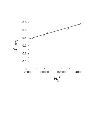
Figure 3: Dependence of $u^{\prime}$ on $R_{\lambda}^{2}$ for a grid-turbulence experiment gm . The straight line indicates Eq. (36).

V Stability

It follows from Eq. (33) that its right hand side should be positive. It can be obtained for any sign of $\beta$ if one chooses an appropriate sign in (34). Therefore, the supercritical and subcritical secondary oscillations co-exist at the multimode bifurcation (while at the standard one-mode Landau-Hopf bifurcations this cannot be possible). This co-existence makes the question about stability of the secondary regimes rather important.

Let us consider the evolutionary equation linearized on the secondary regime

$$(\omega_{0}+\delta\omega)\frac{da_{j}}{d\Theta}=(\beta\delta+\gamma_{j}\omega_{0})a_{j}+$$

$$+\delta\sum_{k,m=1}^{4}b_{jkm}(a_{k}^{(1)}a_{m}+a_{m}^{(1)}a_{k})$$

where $a_{k}^{(1)}(\Theta)$ are the first order (on the parameter $\delta$) modes of the considered secondary oscillations. The Floquet representation for evolutionary operator of these equations is dk

$$\hat{V}(\Theta)=\hat{Q}(\Theta)\exp(\hat{G}\Theta).$$

Stability or instability of the secondary oscillation is determined by spectrum of the operator $\hat{G}$. We use small parameter $\delta$ to find when the spectrum of the operator $\hat{G}$ has its points located in the right semi-plane. Let us expend operator $\hat{G}$

$$\hat{G}=\hat{G}_{0}+\delta\hat{G}_{1}+...$$

where

$$\hat{G}_{0}=i~{}diag\{1,2\}$$

Eigenvalues of the operator $\hat{G}_{0}$ are: $\sigma_{1}^{(0)}=i$ and $\sigma_{2}^{(0)}=2i$. Corresponding eigenvectors are: $x_{1}=(1,0)$, $x_{2}=(0,1)$. To find operator $\hat{G}_{1}$ we use the Krein representation dk

$$\hat{G}_{1}=\frac{1}{4\pi^{2}}\int_{0}^{T_{0}}\oint_{\Gamma_{0}}\oint_{\Gamma_{0}}\frac{(\lambda-\mu)e^{(\mu-\lambda)\tau}}{1-e^{(\mu-\lambda)\tau}}\times$$

$$\times(\hat{G}_{0}-\lambda\hat{I})^{-1}\hat{R}_{1}(\hat{G}_{0}-\mu\hat{I})^{-1}d\tau d\lambda d\mu$$

where $T_{0}=2\pi\omega_{0}^{-1}$,

$$\hat{R}_{1}=\omega_{0}^{-1}diag\{\beta-i\omega_{1},~{}~{}~{}\beta-2i\omega_{1}\}$$

and $\Gamma_{0}$ is a contour enveloping the spectrum of the operator $\hat{G}_{0}$. Harmonic perturbations of the right hand side of the evolutionary equation do not give a contribution to the $\Re\{\sigma\}\sim\delta$. If we now expand spectrum of the operator $\hat{G}$: $\sigma=\sigma^{(0)}+\delta\sigma^{(1)}+...$, then we obtain

$$\sigma^{(1)}=(y,\hat{G}_{1}x)$$

where $x$ is eigenvalue of the operator $\hat{G}_{0}$, $y$ is eigenvalue of the operator conjugate to $\hat{G}_{0}$ and $(,)$ means scalar multiplication. Then, substituting $\hat{G}_{1}$ from (41) into (42) and calculating the integrals we obtain

$$\Re\{\sigma\}=-\beta\omega_{0}^{-1}\delta+...$$

Therefore, for small $\delta$ the subcritical secondary oscillations $(\beta=-1)$ are unstable ($\Re\{\sigma\}>0)$, whereas supercritical ($\beta=1$) secondary oscillations are stable ($\Re\{\sigma\}<0$).

While one-mode equation (19) is two-dimensional (for real variables) the multimode equations are multidimensional: two-mode equation has dimensionality 4, and the three-mode equation for the modes with $\omega_{0}$, $(n-1)\omega_{0}$ and $n\omega_{0}$ has dimensionality 6. It is well known that nonlinear equations with dimensionality larger than 2 and equations with dimensionality smaller (or equal) than 2 have very different properties. In particular, the former equations can generate stochastic attractors. These attractors have considerable capacity in the phase space that allows them to survive in the turbulent environment.

- (1) T. Gotoh, D. Fukayama, and T. Nakano, Phys. Fluids 14 (2002) 1065.
- (2) T. Ishihara, Y. Kaneda, M. Yokokawa, K. Itakura, and A. Uno, J. Phys. Soc. Jpn. 74 (2005) 1464 .
- (3) J. Schumacher, K. R. Sreenivasan, and V. Yakhot, New Journal of Physics 9 (2007) 89.
- (4) P. Mininni, A. Alexakis, A. Pouquet, Phys. Rev. E, 77 (2008) 036306.
- (5) A. Bershadskii, Phys. Fluids, 20 (2008) 085103.
- (6) G. Falkovich, Phys. Fluids, 6 (1994) 1411.
- (7) D. Lohse and A. Muller-Groeling, Phys. Rev. Lett. 74 (1995) 1747.
- (8) A. Bershadskii, J. Stat. Phys., 128 (2007) 721.
- (9) L. Biferale, Phys. Fluids, 20 (2008) 031703.
- (10) L.D. Landau and E.M. Lifshitz, Fluid mechanics (Pergamon, Oxford, 1987).
- (11) J. Guckenheimer and P. Holmes, Nonlinear Oscillations, Dynamical Systems and Bifurcations of Vector Fields (Springer-Verlag, NY, 1983).
- (12) A. Ibetson and D.J. Tritton, J.Fluid Mech., 68 (1975) 639.
- (13) E.J. Hopfinger, R.W. Griffits and M. Mory, J. de Mec., 2 (1983) 21.
- (14) O.M. Phillips, Phys. Fluids, 6 (1963) 513.
- (15) J.O. Hinze, Turbulence, (McGraw-Hill, 1959).
- (16) D. Lohse, Phys. Rev. Lett., 73 (1994) 3223.
- (17) G.L. Eyink, and K.R. Sreenivasan, Rev. Mod. Phys., 78 (2006) 87.
- (18) R.B. Pelz, and Y. Gulak, Phys. Rev. Lett. 25 (1997) 4998.
- (19) R.B. Pelz, Fluid Dynam. Res., 33 (2003) 207.
- (20) P.E. Dimotakis, J. Fluid Mech. 409 (2000) 69.
- (21) K.R. Sreenivasan, A unified view of the origin and morphology of the turbulent boundary layer structure, In Turbulence Management and Relaminarization , 37-61, (ed. H.W. Leipman, R. Narasimha, Springer-Verlag Berlin, 1988).
- (22) S.J. Cowley, Laminar Boundary-Layer Theory: A 20TH century paradox? in Proceedings of ICTAM 2000, eds. H. Aref and J.W. Phillips, 389-411, Kluwer (2001).
- (23) Y. Ponty, J.-P. Laval, B. Dubrulle, F. Daviaud, and J.-F. Pinton, Phys. Rev. Lett., 99 224501 (2007).
- (24) N. Leprovosta and B. Dubrulle, Eur. Phys. J. B, 44, 395 (2005).
- (25) I. Gochberg and M.G. Krein, Introduction to the theory of linear nonselfadjoint operators (Am. Math. Soc., NY, 1969).
- (26) S. Cerutti and C. Meneveau, Phys. Fluids, 12 (2000) 1143.
- (27) Yu.L. Daletskii and M.G. Krein, Stability of solutions of differential equations in Banach space (Am. Math. Soc., NY, 1974).