Particle trajectories and acceleration during 3D fan reconnection

Abstract

Context. The primary energy release in solar flares is almost certainly due to magnetic reconnection, making this a strong candidate as a mechanism for particle acceleration. While particle acceleration in 2D geometries has been widely studied, investigations in 3D are a recent development. Two main classes of reconnection regimes at a 3D magnetic null point have been identified: fan and spine reconnection

Aims. Here we investigate particle trajectories and acceleration during reconnection at a 3D null point, using a test particle numerical code, and compare the efficiency of the fan and spine regimes in generating an energetic particle population.

Methods. We calculated the time evolution of the energy spectra. We discuss the geometry of particle escape from the two configurations and characterise the trapped and escaped populations.

Results. We find that fan reconnection is less efficent than spine reconnection in providing seed particles to the region of strong electric field where acceleration is possible. The establishment of a steady-state spectrum requires approximately double the time in fan reconnection. The steady-state energy spectrum at intermediate energies (protons 1 keV to 0.1 MeV) is comparable in the fan and spine regimes. While in spine reconnection particle escape takes place in two symmetric jets along the spine, in fan reconnection no jets are produced and particles escape in the fan plane, in a ribbon-like structure.

1 Introduction

In recent years, magnetic reconnection has been recognised as the key process underlying energy release in solar flares. At the same time, the importance of generalising the well established 2D reconnection theory to 3D configurations has been emphasised by many authors. Reconnection in 3D can take place in various locations, including separator lines; but in initial studies, it is natural to focus on the simplest configuration, which is also the closest analogue of the classic 2D X-point, namely a 3D magnetic null. Such null points are likely to be common in the solar corona, due to the complex topology arising from the mixed polarity photospheric flux sources [Schrijver and Title (2002); Longcope et. al. (2003)]. The SOHO EIT images have given direct evidence of a 3D null in a solar coronal Active Region [Filippov (1999)] and reconstructions of the solar magnetic fields of active regions have shown that reconnecting 3D nulls can be present during solar flares [Aulanier et al. (2000); Fletcher et al. (2001)]. Recently, Cluster has found a 3D null point in a reconnection event in the Earth’s magnetotail [Xiao et al. (2006)].

One important consequence of reconnection is the acceleration of charged particles by the strong electric fields associated with the process. As confirmed by recent results from RHESSI [Lin et. al. (2003)], large numbers of nonthermal electrons and protons are observed in solar flares. It is an attractive hypothesis that magnetic reconnection, the primary source of the energy release, is also responsible for generating these high energy particles. Particle acceleration by reconnection has been extensively studied in 2D, and 2D models are continously being improved (see Hannah and Fletcher (2006) and references therein). However, very little is known about particle acceleration in 3D geometries, although these should be common in nature, and the idealisations of 2D models may lead to unrealistic results (for example, a 2D configuration has an electric field of infinite spatial extent in the invariant direction along a line of points in which the magnetic field is zero). Some interesting preliminary studies have been undertaken of test particles using 3D MHD codes to provide background electromagnetic fields [Schopper et. al. (1999); Turkmani et, al. (2005, 2006)], but these are limited by numerical resolution and it is difficult to derive an understanding of scaling or general properties. Recently, we began to study the fundamental properties of particle acceleration in 3D by considering a basic 3D null point geometry [Dalla and Browning (2005, 2006)].

Two regimes of reconnection at a 3D magnetic null are possible: spine and fan reconnection [Lau and Finn (1990); Priest and Titov (1996)]. While the magnetic field configuration is the same in the two regimes, they are characterised by different plasma flow patterns and different electric fields. Spine reconnection has a current concentration along the critical spine field line, while fan reconnection has a current sheet in the fan plane.

In previous work we focussed on the spine reconnection regime, and analysed the trajectories of single particles, as well as the evolution of the spectrum and spatial distributions of a population of particles [Dalla and Browning (2005, 2006)]. We found that the 3D spine reconnection regime can be an efficient particle accelerator and that particles escaping from the region near the null, do so in two symmetric jets along the spine.

In this paper we focus on the 3D fan reconnection regime, with specific interest in comparing the efficiency of fan and spine reconnection in providing seed particles for acceleration to the regions of strong electric fields, and in studying the 3D geometry of particle escape after acceleration. We study this problem within the test particle approach, by means of a numerical code in which the trajectories of a particle population are numerically integrated.

We adopt the Priest and Titov (1996) model of fan reconnection. This model applies to the outer ideal reconnection region and does not include acceleration due to the parallel electric field in the inner dissipation (resistive) region; indeed, the mathematical model breaks down very close to the spine/fan as the electric field formally diverges (in our code, we eliminate this singularity as described in Sec. 2 below). Despite its limitations, there are advantages to having a relatively simple field model which highlights key topological and geometrical properties; the Priest and Titov (1996) model is the closest 3D analogue to the constant out-of-plane electric field ($E_{z}$) which is very widely used in 2D particle acceleration models [eg: Deeg et al. (1991); Vekstein and Browning (1997); Fletcher and Petkaki (1997); Hannah and Fletcher (2006)]. The use of a constant $E_{z}$ also excludes the direct parallel electric field acceleration (at least in the case of zero guide field) and is not a self-consistent reconnection solution in general. It is important to understand the 3D analogue of the well studied 2D problem, before investigating more complete but inevitably much more complex models. Moreover 2D models with more complex fields show good agreement with simplified models based on inflow to neutral point.

It should also be noted that in a highly conducting plasma, the size of the dissipative region will be very small in spatial extent. The majority of particles in a volume that includes a dissipation region (a current sheet at the fan plane in fan reconnection) will not enter such a region at all. We plan to include dissipative effects in future work. Our work here is thus complementary to that of Litvinenko (2006), who considers, using an approximate analytical approach, only the acceleration of particles due to the parallel electric field within the fan plane current sheet. As has been shown by Vekstein and Browning (1997), electric fields outside the dissipation region contribute to the acceleration as well as determining the way in which particles are supplied to the small resistive region. The full trajectory approach that we use (as opposed to the guiding center approach) can properly describe the acceleration that occurs as particles reach the region in the vicinity of the fan plane region where the electric field is strong and the guiding center approximation breaks down.

The reconnection configuration is outlined in Section 2. Results are presented in Sections 3 and 4, which consider respectively single particle trajectories and distributions of particles. The conclusions are presented in Section 5.

2 Fan reconnection configuration

We consider a magnetic configuration of the form:

$$B_{x} = B_{0}\,x$$ (1)

$$B_{y} = B_{0}\,y$$ (2)

$$B_{z} = -2\,B_{0}\,z$$ (3)

describing a potential 3D magnetic null, where the spatial variables $x$, $y$ and $z$ are normalised with respect to a length $L$, the size of the simulation box, which represents a global length scale. Here $B_{0}$ is the magnitude of ${\bf B}$ at $\sqrt{(x^{2}+y^{2})}$=1 and $z$=0. It should be noted that this current-free null is the simplest of a family of 3D nulls (Parnell et. al. (1996)), but it is used because analytical expressions for the electric field in a reconnection situation are available, as discussed below. For our potential magnetic null, an axis of symmetry of the magnetic field, called the spine, is present, labelled here as the $z$ axis. This critical fieldline connects to the null point. In the plane $z$=0, the magnetic field lines are straight lines through the null point, describing a fan. Hence this plane is called the fan plane. The spine and the fan are the 3D analogues of the separatrix planes in classic 2D X-point geometry.

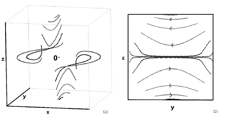
Figure 1: Diagrams of flow lines for 3D fan reconnection: (a) 3D graph of flow lines; (b) Projection of the flow lines onto the $y$-$z$ plane.

Reconnection regimes at a 3D magnetic null have been described by Lau and Finn (1990) and Priest and Titov (1996). Two types of reconnection are possible: spine and fan reconnection. We have previously studied the spine mode [Dalla and Browning (2005, 2006)], hence the focus here is on fan reconnection. For a potential null, the spine reconnection regime is characterised by plasma flows lying in planes containing the spine, while fan reconnection has non-planar flows that carry the magnetic field lines in a ‘swirling’-like motion anti-symmetric about the fan plane. The fan plane is thus a singular surface as the flow is discontinous. The specific flow pattern of the model we use, results from having imposed, on surfaces at $z$=$+$1 and $z$=$-$1, that the plasma flow is along straight lines parallel to the to the $y$-axis and its magnitude only depends on $y$ [Priest and Titov (1996)]. In other words, on the chosen surfaces: $v_{x}$=$v_{z}$=0 and $v_{y}$=$v_{y}(y)$, with $v$ the plasma flow velocity. Note that the resulting electric field and flow pattern are non-axisymmetric, and that these are not unique, but only one of the possible solutions that give rise to fan reconnection. Imposing the above flows introduces a preferential direction, the $y$ axis in our geometry, and this will control the particles’ behaviour, as shown in Sections 3 and 4. Other types of fan reconnection will similarly be characterised by a preferential direction, so in this sense our results are generic.

The electric field we consider was derived by Priest and Titov (1996) and has the expression:

$$E_{x} = E_{0}\>\frac{-\,|z|^{1/2}}{(4+y^{2}\,|z|)^{1/2}}$$ (4)

$$E_{y} = E_{0}\>\frac{xy\,|z|^{3/2}}{(4+y^{2}\,|z|)^{3/2}}$$ (5)

$$E_{z} = E_{0}\>\frac{-2x\>\mbox{sign}\,z\>|z|^{-1/2}}{(4+y^{2}\,|z|)^{3/2}}$$ (6)

where $\mbox{sign}\,z$=1 if $z$$>$$0$ and $\mbox{sign}\,z$=$-$1 if $z$$<$$0$.

Figure 1 shows diagrams representing the plasma flow lines during fan reconnection in the Priest and Titov model. Figure 1-(a) gives a 3D view of flows for plasma parcels starting in a plane containing the spine, at a value of the azimuthal angle $\phi$=100^∘; Figure 1-(b) shows a projection of the flow lines onto the $y$-$z$ plane. The azimuthal angle (longitude) is defined as $\phi$=$\tan^{-1}(y/x)$, and the latitude $\beta$ as $\beta$=$\tan^{-1}(z/\sqrt{x^{2}+y^{2}})$.

The electric field given by Eqs. (4)–(6) is characterised by a singularity in the fan plane, i.e.  when $z$=0. We eliminate this singularity by replacing, in Eq. (6): $|z|^{-1/2}$ by $z\,(z^{2}+l^{2})^{-3/4}$, with $l$ a small constant giving the length scale of the dissipative layer in which resistivity (or other dissipative effects) are significant. Hence $l$ can be taken to represent the width of the current sheet. In future, the singularity will be resolved more realistically by using self-consistent reconnection models incorporating a localised dissipation region at the fan plane.

3 Single particle trajectories

We first analyse trajectories of a single particle in the 3D fan reconnection configuration, by numerically integrating the equations of motion with the electric and magnetic fields given by eqs.(1)–(6). We solve the relativistic equations of motions given by:

$$\frac{d{\bf x}}{dt} = \frac{{\bf p}}{m_{0}\gamma}$$ (7)

$$\frac{d{\bf p}}{dt} = q\,\left({\bf E}+\frac{1}{c}\frac{{\bf p}}{m_{0}\gamma}\times{\bf B}\right)$$ (8)

where $t$ is time, ${\bf x}$ and ${\bf p}$ are the particle’s position and momentum, $q$ and $m_{0}$ its charge and rest mass, $\gamma$ its relativistic factor, and $c$ is the speed of light.

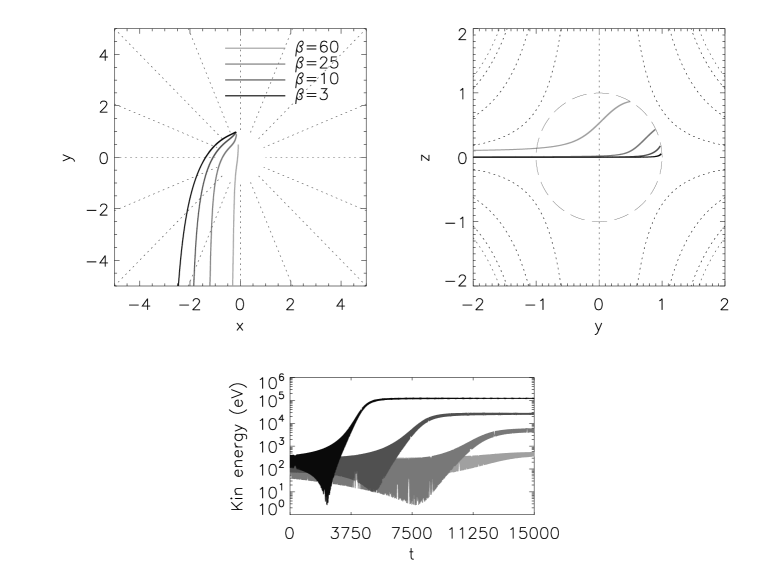
Figure 2: Single particle trajectories in the 3D fan reconnection configuration, for initial positions at $r$=1, longitude $\phi$=100^∘ and latitudes $\beta$=60^∘, 25^∘, 10^∘, 3^∘. The initial particle energy is 300 eV. The particle is a proton with initial pitch angle 92^∘. We use $E_{0}$=3 kV/m, $B_{0}$=100 gauss, L=10 km, t_final=15000. Dotted lines indicate projections of magnetic field lines.

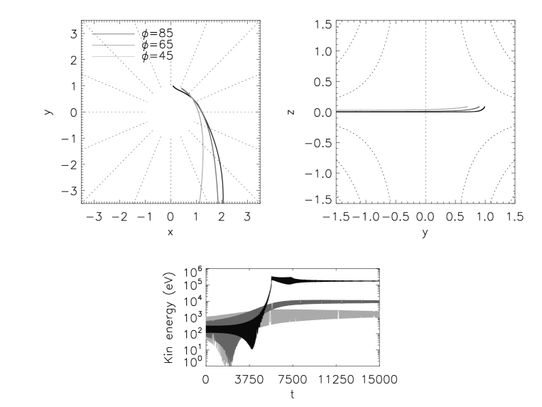
Figure 3: Single particle trajectories in the 3D fan reconnection configuration, for initial positions at $r$=1, constant latitude $\beta$=5^∘ and azimuthal angles $\phi$=85^∘, 65^∘, 45^∘. The other input parameters are the same as in Figure 2.

We normalise distances by the characteristic length $L$, the magnetic field by $B_{0}$, and times by the nonrelativistic gyroperiod associated with a magnetic field of magnitude $B_{0}$: $T=2\pi m_{0}c/(|q|B_{0})$.

The value of the electric field magnitude $E_{0}$ is an input parameter to our numerical code. In order to compare the efficiency of acceleration in fan and spine reconnection, we choose $E_{0}$ in such a way that the average value of $|\@vec{E}|$ in a random set of points on a sphere of radius 1 centered in the null point, is the same for the two cases. We find that a value $E_{0}$=0.1025 statvolt/cm $\sim$3 kV/m corresponds to the same average electric field on the sphere as we used in our previous spine reconnection work [Dalla and Browning (2005, 2006)]. We choose the parameter $l$, defined in Section 2, to have a value 10^-5: we verified that the same results are obtained when a value 10 times smaller is chosen. We use $B_{0}$=100 gauss and L=10 km. The magnetic field value used is typical of a solar Active Region. The effect of varying these parameters will be described in detail elsewhere [Dalla and Browning, in preparation, 2008]; the typical behaviour is that decreasing the value of $B_{0}$ results in a faster drift of particles towards the region of strong magnetic field and consequently a more efficient acceleration.

In Figure 2 we show three particle trajectories with initial positions in the plane through the spine at $\phi$=100^∘ and three values of the latitude $\beta$ (note that the fan plane corresponds to $\beta$=0). The distance from the null, $r$=$(x^{2}+y^{2}+z^{2})^{1/2}$, is $r$=1 at the initial time. The initial particle energy is 300 eV. There is a strong dependence of the energy gain on the initial value of the latitude, with particles starting near the fan plane gaining the most energy. Particles starting at latitudes greater than about $\beta$$\sim$30^∘ have very little acceleration. While moving towards the fan plane, where the electric field is strong, particles are at the same time moving away from the null point and towards regions of stronger magnetic field, as shown in the $x$-$y$ projection.

In Figure 3 we keep the latitude of the particle’s initial position constant (equal to $\beta$=5^∘), and vary the azimuthal angle. Here we can see that an initial position at $\phi$=85^∘ results in stronger acceleration than one at $\phi$=65^∘, and very little acceleration is achieved if the starting position is at $\phi$=45^∘. The trajectories of Figure 3 can be explained by considering the components of the electric drift velocity:

$$\@vec{v}_{E}=c\,\frac{{\@vec{E}}\times{\@vec{B}}}{B^{2}}$$ (9)

with $\@vec{E}$ and $\@vec{B}$ given by eqs.(1)–(6). Calculating the $z$ component of $\@vec{v}_{E}$ shows that it is largest when $\phi$=90^∘ and it is zero at $\phi$=0^∘. Hence azimuthal locations near $\phi$=90^∘ result in more efficient drift toward the fan plane, where the electric field is large and acceleration is most efficient.

Figures 2 and 3 show that, unlike in spine reconnection, there is strong drift in the azimuthal direction. The only exception to this is the motion of a particle that starts the $y$=0 plane (corresponding to $\phi$=90^∘), for which the motion remains planar. In this plane only, the flow lines resemble those of the spine reconnection case, and particles can cross the fan plane and exit the region near the null at negative latitudes. In all other planes through the spine, particles cannot cross the fan plane.

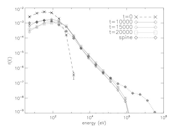
Figure 4: Time evolution of the energy spectrum during fan reconnection with $E_{0}$=3 kV/m, up to a final time $t$=20000. The dotted line gives the spine reconnection spectrum at $t$=10000.

The $x$-$y$ projections in Figures 2 and 3 show a tendency for particles to move parallel to the $y$ axis once they have left the region near the null point. This can be understood by introducing a potential $\psi$ such that ${\bf E}=-\nabla\psi$. From Eqs. (4)–(6) one obtains:

$$\psi(x,y,z)=E_{0}\,L\,\frac{x\,\sqrt{|z|}}{(4+|z|\,y^{2})^{1/2}}$$ (10)

(here $\psi$ is dimensional while $x$, $y$ and $z$ are dimensionless). Conservation of energy requires that the quantity $W$=$K+q\psi$, where $K$ is the kinetic energy, is constant during the motion. When particles are sufficiently far from the null point, their kinetic energy remains approximately constant, as can be seen in the lower panels of Figure 2 and Figure 3, therefore conservation of energy implies that $\psi(x,y,z)$ must also remain constant. For the trajectories of Figure 2, for example, a constant kinetic energy is achieved for $y$-values ranging from $-$0.2 (for $\beta$=60^∘) to $-$3.9 (for $\beta$=3^∘) (note that the distance of the particle from the fan plane is also a factor in determining when acceleration stops, because at larger distances from this plane the electric field is less strong). At the same time, the value of $z$ is small and slowly decreasing: the values of $z$ at the time when the kinetic energy becomes constant for the Figure 2 trajectories are $z$=0.0004, 0.0019, 0.010 and 0.18 for $\beta$=3^∘, 10^∘, 25^∘ and 60^∘ respectively. From Eq. (10), we can see that a constant $\psi$ and very small $z$ give a tendency for $x$ to remain roughly constant, or in other words for the motion to be approximately parallel to the $y$ axis. This tendency is stronger for particles that get nearer the fan plane: these are also those that achieve largest acceleration. The direction of the $y$ axis is the preferential flow direction within this type of fan reconnection, as described in Section 2.

It is also interesting to look at the properties of the bulk flow velocity $V$ near the plane $z$=0, given, for $z$$>$0, by:

$$V_{x} \sim \frac{x\,y}{4(x^{2}+y^{2})\sqrt{z}}$$ (11)

$$V_{y} \sim \frac{-x^{2}}{4(x^{2}+y^{2})\sqrt{z}}$$ (12)

$$V_{z} \sim \frac{-y\sqrt{z}}{2(x^{2}+y^{2})}$$ (13)

Eqs. (11)–(13) are obtained from Eqs. (4.25) of Priest and Titov (1996), by taking the limit $z$$\rightarrow$0 (with our equations having opposite sign to Priest and Titov (1996) to ensure that ${\bf E}=-\nabla\psi$). Near the fan plane, the $V_{z}$ component is small so that particles tend to remain near this plane. The streamlines in the fan plane are approximately circles (see Figure 1-a). The drift velocity is generally directed from the positive $y$ quadrant to negative $y$, with a strong flow in the negative $y$ direction across the $x$-axis; this also shows that particles tend to pick up a velocity anti-parallel to the $y$ axis. Furthermore, particles starting closer to the positive $y$ axis (at larger $\phi$) remain in the swirling stream for longer time, and so gain more energy (see Figure 3).

4 Particle spatial distributions and spectra

To analyse the evolution of a population of particles during fan reconnection, we inject 10000 protons at random positions on a sphere of radius 1 around the null point, in the same way as done by Dalla and Browning (2006) for spine reconnection.

Figure 4 shows the time evolution of the energy spectrum, for 10000 protons with initial Maxwellian energy distribution with temperature = 10⁶K. We find that in order to reach a steady-state spectrum, we need to integrate particle trajectories up to a normalised time $t$=20000, approximately double the time that was required to reach a steady-state during spine reconnection for the same parameters. The dotted line shows the steady-state energy spectrum from the spine reconnection analysis Dalla and Browning (2006), at the final time $t$=10000. Comparison of the fan and spine plots at the final times shows that spine reconnection produces a larger population of high energy particles (protons above 0.1 MeV).

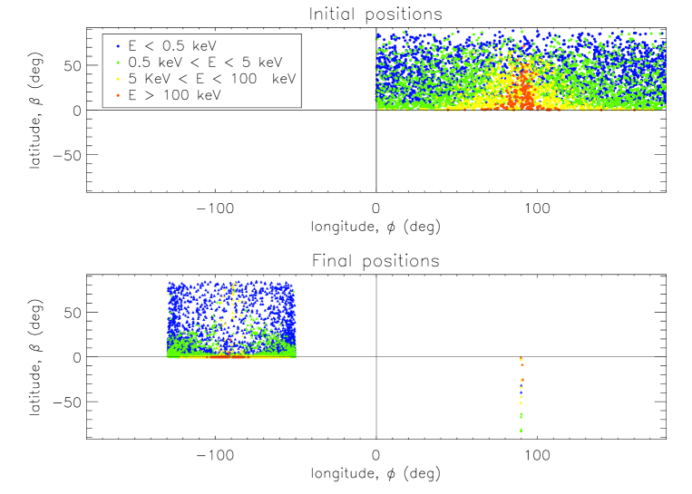
Figure 5: Initial and final positions of particles during fan reconnection at the initial time t=0 (top) and final time t=20000 (bottom).

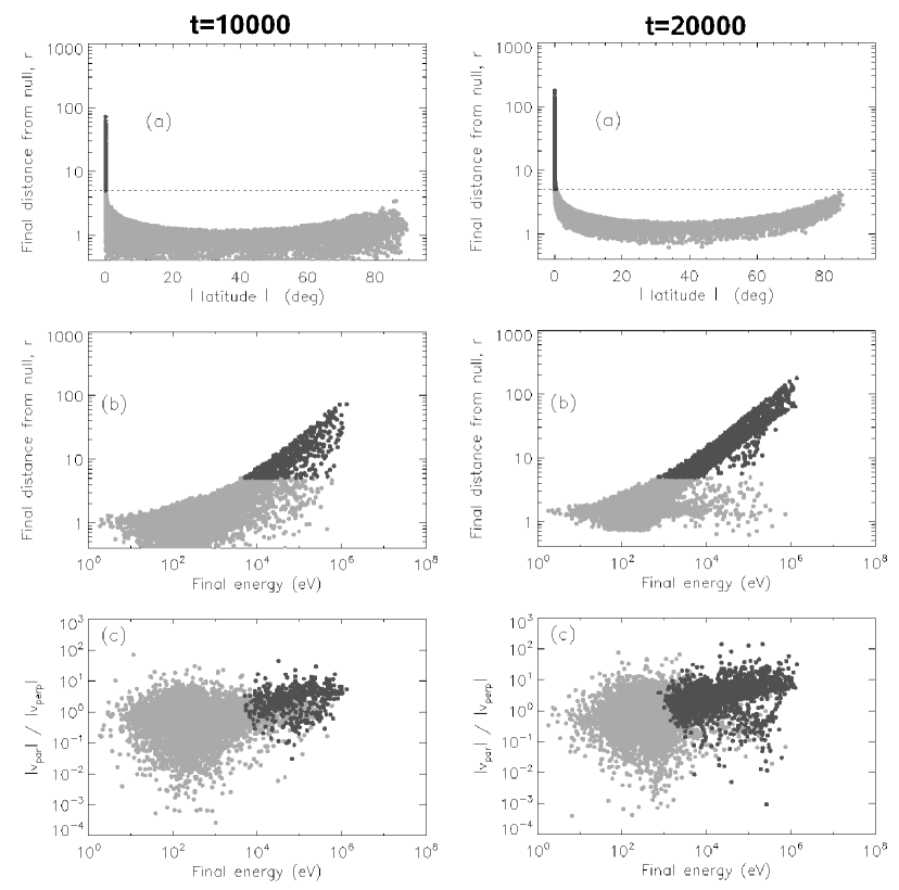
Figure 6: Parameters of the energetic particle populations during fan reconnection at $t$=10000 (left) and $t$=20000 (right). (a) Distance from the null versus absolute value of latitude at the given time. (b) Distance from the null versus particle energy. (c) Ratio of the magnitude of the component of velocity parallel to the magnetic field to perpendicular component, versus particle energy. Dark grey points indicate particles with $r$$>$5 and small $|\beta|$, light grey points all the other particles.

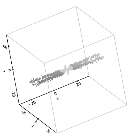
Figure 7: 3D view of particles at t=20000, for particles within a cube of size 30 centered on the null. The colour coding is the same as in Figure 6, showing in dark grey particles with $r$$>$5. These are are escaping in a ribbon-like configuration.

In the intermediate energy range (protons 1 keV to 0.1 MeV), the efficiency of fan and spine reconnection is similar once a steady state is reached. The slope of the curve is very similar in this energy range, hence so is the power law index of the spectra.

Figure 5 shows the angular location of the particles in our population at the initial time (top plot) and the final time (bottom plot). Each location is identified by its latitude $\beta$, i.e. the elevation angle from the $x$-$y$ plane, and longitude $\phi$. Inflow regions are the top-right and bottom-left quadrants in the $\phi$, $\beta$ representation. In Figure 5 we only show the initial and final positions of particles starting in the top-right inflow region. Particles (not shown) starting in the bottom left quadrant have distributions of initial and final positions symmetric with respect to those shown in Figure 5, apart from statistical fluctuations. Each point of Figure 5 represents one particle and is colour coded according to the final particle energy. It should be noted that the energy ranges corresponding to the various colours are different from those used in Dalla and Browning (2006), since the maximum particle energies obtained in fan reconnection are lower than in spine reconnection.

Figure 5 shows that particles starting near the fan plane are those that gain the largest energy, as would be expected since the fan plane is the location where the electric field is largest. As one moves towards increasing latitudes, particles will reach the fan plane with greater difficulty and gain less energy. Figure 5 shows that at the final time, particles are confined to a range of longitudes [$-$130^∘,$-$50^∘] (and symmetrically for negative latitudes, not shown in Figure 5, longitudes [50^∘,130^∘]). This is a result of the tendency of particles to move anti-parallel to the $y$ axis after they have passed the region near the null, as discussed in Sec. 3. This is clearly shown in Figure 3, in which particles with initial positions covering a wide range of azimuthal angles $\phi$, leave the null moving anti-parallel to the $y$ axis and within a narrower band of $\phi$.

Figure 5 also shows that initial azimuthal locations near $\phi$=90^∘ are the most favourable for particle acceleration since near this plane the $z$ component of the electric field drift, pushing particles towards the fan plane, is largest. Furthermore, such particles spend longest in the swirling flows, as shown in Figure 3.

In Dalla and Browning (2006) we reported that the spine reconnection configuration naturally produces two symmetric jets of energetic particles escaping along the spine. The escaping particles in the two jets were found at large distances from the null point at the final time.

Figure 6 adds information about the distance from the null point at the final time, to the angular information displayed in Figure 5. Figure 6 displays a snapshot of the same information at $t$=10000 (left panels) and $t$=20000 (right panels). Panels (a) show the distance from the null point versus magnitude of the latitude $\beta$. No particles are found at values of $|\beta|$ near 90^∘, i.e. no particles are escaping along the spine during fan reconnection.

However some particles are escaping from the configuration after acceleration: they are represented in Figure 6 by the dark grey points found at low $|\beta|$, i.e. near the fan plane. The same particles found around $r$=50 at $t$=10000 are found at approximately $r$=100 at $t$=20000. These particles have energies in the range 10 keV to 1 Mev at $t$=20000 (panel (b)) and are characterised by a ratio of the parallel to perpendicular component of velocity greater than 1 (panel (c)). Consequently they are escaping from the magnetic configuration.

Figure 7 gives a 3D view of the escaping population, showing that they are moving away from the magnetic null in a ribbon like structure. The orientation of the ribbon is parallel to the direction along which the fan reconnection flows have been imposed (the $y$ axis in our reference system).

5 Conclusions

In this work we analysed test particle trajectories in the fields characteristic of fan reconnection, one of the two regimes of magnetic reconnection at a 3D magnetic null. We aimed to investigate how efficiently particles can reach the region of strong electric field where acceleration is possible, and the geometry of particle escape after acceleration has taken place. Also, we assessed the differences between the fan regime and the previously studied spine reconnection one.

We found that the fan reconnection regime is less efficient in seeding test particles to the region of strong electric field, compared to the spine reconnection one. The time required for acceleration to take place is approximately twice the one we previously found for the spine regime [Dalla and Browning (2006)]. This is due to the flow patterns for fan reconnection making it difficult for particles starting at high latitude locations to reach the fan plane, where the electric field is large.

The steady-state spectrum we obtained for fan reconnection has a spectral index in the intermediate energy range (protons 1 keV to 0.1 MeV, for the parameters used in our study) that is similar to the spine case one. However, within our model, it appears that fan reconnection is less efficient in the generation of a very high energy population (protons $>$0.1 MeV), compared to the spine case. It should be emphasised that our model, based on the Priest and Titov (1996) formulation, does not accurately represent the small region where resistive (or other dissipative) effects become important. Our statement regarding the maximum particle energy produced by each of the two regimes will need to be re-assessed within a model including parallel electric fields within the resistive region, and which properly models the ”cut off” of the ideal electric field as this region is approached. This will be the subject of future study. However, our model does properly represent the inflow of particles to the dissipative region where parallel electric fields exist. Hence, only those particles reaching the fan plane (the high energy tail in our calculation) may be further accelerated to even higher energies. We thus expect that using a more self-consistent reconnection model will affect only the high energy tail and cut-off of the energy spectra.

Regarding the geometry of escape from the region near the null after acceleration, we found that in the fan reconnection case energetic particles escape along the fan plane in a ribbon-like configuration. We do not observe particle escape along the spine line, as was the case in the spine regime [Dalla and Browning (2006)]. Thus, in principle, observations of the spatial distribution of high energy particles might be a discriminator between spine and fan reconnection.