Spectral evolution of superluminal components in parsec-scale jets

Abstract

We present numerical simulations of the spectral evolution and emission of radio components in relativistic jets. We compute jet models by means of a relativistic hydrodynamics code. We have developed an algorithm (SPEV) for the transport of a population of non-thermal electrons including radiative losses. For large values of the ratio of gas pressure to magnetic field energy density, $\alpha_{{}_{\rm B}}\sim 6\times 10^{4}$, quiescent jet models show substantial spectral evolution, with observational consequences only above radio frequencies. Larger values of the magnetic field ($\alpha_{{}_{\rm B}}\sim 6\times 10^{2}$), such that synchrotron losses are moderately important at radio frequencies, present a larger ratio of shocked-to-unshocked regions brightness than the models without radiative losses, despite the fact that they correspond to the same underlying hydrodynamic structure. We also show that jets with a positive photon spectral index result if the lower limit $\gamma_{\rm min}$ of the non-thermal particle energy distribution is large enough. A temporary increase of the Lorentz factor at the jet inlet produces a traveling perturbation that appears in the synthetic maps as a superluminal component. We show that trailing components can be originated not only in pressure matched jets, but also in over-pressured ones, where the existence of recollimation shocks does not allow for a direct identification of such features as Kelvin-Helmholtz modes, and its observational imprint depends on the observing frequency. If the magnetic field is large ($\alpha_{{}_{\rm B}}\sim 6\times 10^{2}$), the spectral index in the rarefaction trailing the traveling perturbation does not change much with respect to the same model without any hydrodynamic perturbation. If the synchrotron losses are considered the spectral index displays a smaller value than in the corresponding region of the quiescent jet model.

1. Introduction

Relativistic jets are routinely observed emerging from active galactic nuclei and microquasars, and presumably they are behind the phenomenology detected in gamma-ray bursts. It is a broadly recognized fact that the observed VLBI radio-maps of parsec-scale jets are not a direct map of the physical state (density, pressure, velocity, magnetic field) of the emitting plasma. The emission structure is greatly modified by the fact that a distant (Earth) observer detects the radiation emitted from a jet which moves at relativistic speed and forms a certain angle with respect to the line of sight. Time delays between different emitting regions, Doppler boosting and light aberration shape decisively the observed aspect of every time-dependent process in the jet. The observed patterns are also influenced by the travel path of the emitted radiation towards the observer since Faraday rotation and, most importantly, opacity modulate total intensity and polarization radio maps. Finally, there are other effects that can be very important for shaping VLBI observations which do not unambiguously depend on the hydrodynamic jet structure, namely, radiative losses, particle acceleration at shocks, pair formation, etc. In this work we try to account for some of these elements by means of numerical simulations.

The basis for currently accepted interpretation of the phenomenology of relativistic jets was set by Blandford & Königl (1979) and Königl (1981). A number of analytic works have settled the basic understanding that accounts for the non-thermal synchrotron and inverse Compton emission of extragalactic jets (e.g., Marscher, 1980), as well as the spectral evolution of superluminal components in parsec-scale jets (e.g., Blandford & McKee, 1976; Hughes, Aller & Aller, 1985; Marscher, Gear & Travis, 1992; Marscher & Gear, 1985). Assuming kinematic jet models, the numerical implementation of these analytic results enables one to extensively test the most critical theoretical assumptions by comparison with the observed phenomenology both for steady (e.g., Daly & Marscher, 1988; Hughes, Aller & Aller, 1989a, 1991; Gómez, Alberdi & Marcaide, 1993, 1994; Gómez, et al., 1994) and unsteady jets (e.g., Jones, 1988). Basically, the aforementioned numerical implementation consists on integrating the synchrotron transfer equations assuming that radiation originated from an idealized jet model and accounting for all the effects mentioned in the previous paragraph.

The advent of multidimensional relativistic (magneto-)hydrodynamic numerical codes has allowed to replace the previously used kinematic, steady jet models by multidimensional, time-dependent hydrodynamic models of thermal plasmas (for a review see, e.g., Gómez, 2002). The works of Gómez, et al. (1995, 1997), (hereafter G95 and G97, respectively) Duncan, Hughes & Opperman (1996) or Komissarov & Falle (1996) compute the synchrotron emission of relativistic hydrodynamic jet models with suitable algorithms that account for a number of relativistic effects (e.g., Doppler boosting, light aberration, time delays, etc.). Their models assume that there exists a proportionality between the number and the energy density of the hydrodynamic (thermal) plasma and the corresponding number and energy density of the emitting population of non-thermal or supra-thermal particles. These authors assumed that the magnetic field was dynamically negligible, that the emitted radiation had no back-reaction on the dynamics, and that that synchrotron losses were negligible. All these assumptions are very reasonable for VLBI jets at radio observing frequencies if the jet magnetic field is sufficiently weak. Consistent with their assumptions, the former papers included neither a consistent spectral evolution of the non-thermal particle (NTP) population, nor the proper particle and energy transport along the jet.

The spectral evolution of NTPs and its transport in classical jets and radiogalaxies have been carried out by Jones, Ryu & Engel (1999), Micono, et al. (1999) and Tregillis, Jones & Ryu (2001). In these works a coupled evolution of a non-relativistic plasma along with a population of NTPs has been used to asses either the signatures of diffusive shock acceleration in radio galaxies (Jones, Ryu & Engel, 1999; Tregillis, Jones & Ryu, 2001) or the observational imprint of the non-linear saturation of Kelvin-Helmholtz (KH) modes developed by a perturbed beam (Micono, et al., 1999). Casse & Marcowith (2003) have also developed a scheme to perform multidimensional Newtonian magneto-hydrodynamical simulations coupled with stochastic differential equations adapted to test particle acceleration and transport in kilo-parsec scale jets. Dealing with the spectral evolution of NTPs is relevant in view of the multiband observations of extragalactic jets where, a significant aging of the emitting particles seems to be present at optical to X-ray frequencies (M87, Heinz & Begelman, 1997; Marshall, et al., 2002; Cen A, Kraft, Forman, Jones & Murray, 2001).

This paper builds upon the lines opened by G95 and G97. G95 concentrated on the emission properties from steady relativistic jets, focusing on the role played by the external medium in determining the jet opening angle and presence of standing shocks. G97 used a similar numerical procedure to study the ejection, structure, and evolution of superluminal components through variations in the ejection velocity at the jet inlet. Agudo et al. (2001) discussed in detail how a single hydrodynamic perturbation triggers pinch body modes in a relativistic, axisymmetric beam which result in observable superluminal features trailing the main superluminal component. Finally, Aloy, et al. (2003) extended the work of Agudo et al. (2001) to three-dimensional, helically perturbed beams. Here, we combine multidimensional relativistic models of compact jets with a new algorithm to compute the spectral evolution of supra-thermal particles evolving in its bosom, i.e., including their radiative losses, and their relevance for the emission and the spectral study of relativistic jets.

This work is composed of two parts. In the first part, we present a new numerical scheme to evolve populations of relativistic electrons in relativistic hydrodynamical flows including radiative losses (§ 3). For the purpose of calibration the new method, our work is based upon the same axisymmetric, relativistic, hydrodynamic jet models as employed in G97. Using the same jet parameters allows us to quantify the relevance of including radiative losses and, along the way, to compare the emission properties of parsec-scale jets computed according to two different methods: (1) the new method presented in this paper and (2) the method presented in G95 and G97, to which we will refer, for simplicity, as Adiabatic Method (AM). In the second part of the paper, we apply the new method to quantify the relevance of radiative losses in the evolution of both quiescent and dynamical jet models. We will show (§ 5) the regimes in which both approaches yield similar synthetic total intensity radio maps and when synchrotron losses modify substantially the results. We also show which are the key parameters to trigger a substantial NTP aging and, therefore, to significantly change the appearance of the radio maps corresponding to the same underlying, quiescent jet models. The spectral evolution of a hydrodynamic perturbation travelling downstream the jet, will be discussed in Sect. 7. Finally, we discuss our main results and conclusions in Sect. 8.

2. Hydrodynamic models

Table 1Set of models used in this work. Values in the table refer to the jet nozzle. The first column lists the model names. The second and third columns give the jet-to-external-medium pressure ratio, and the comoving magnetic field at the jet nozzle, respectively. The last column lists the values of the ratio of gas pressure to magnetic pressure. Additional models not including radiative losses, but computed with the SPEV method, will be denoted with a suffix “-NL”. Likewise, models with the same parameters as the ones listed here, but computed with the AM method, will be denoted with a suffix “-AM”.

model	$P_{b}/P_{a}$	$b_{b}$ [G]	$\alpha_{{}_{\rm B}}$
PM-S	1.0	0.002	$6\times 10^{6}$
PM-L	1.0	0.02	$6\times 10^{4}$
PM-H	1.0	0.20	$6\times 10^{2}$
OP-L	1.5	0.03	$6\times 10^{4}$
OP-H	1.5	0.30	$6\times 10^{2}$

Two quiescent, relativistic, axisymmetric jet models constitute our basic hydrodynamic set up (see Tab. 1). They correspond to the same pressure-matched (PM), and over-pressured (OP) models of G97. The models were computed in cylindrical symmetry with the code RGENESIS (Mimica, et al., 2004). The computational domain spans $(10R_{b}\times 200R_{b})$ in the $(r\times z)$-plane ($R_{b}$ is the beam cross-sectional radius at the injection position). A uniform resolution of 8 numerical cells/$R_{b}$ is used. The code module that integrates the relativistic hydrodynamics equations is a conservative, Eulerian implementation of a Godunov-type scheme with high-order spatial and temporal accuracy (based on the GENESIS code; Aloy, et al., 1999; Aloy, Pons & Ibáñez, 1999). We follow the same nomenclature as G97 where quantities affected by subscripts a, b and p refer to variables of the atmosphere, of the beam at the injection nozzle and of the perturbation (§ 2.1), respectively. The jet material is represented by a diffuse ($\rho_{b}/\rho_{a}=10^{-3}$; $\rho$ being the rest-mass density), relativistic (Lorentz factor $\Gamma_{b}=4$) ideal gas of adiabatic exponent $4/3$, with a Mach number $M_{b}=1.69$. At the injection position, model PM has a pressure $P_{b}=P_{a}$, while model OP has $P_{b}=1.5P_{a}$.Pressure in the atmosphere decays with distance $z$ according to $P(z)=P_{a}/[1+(z/z_{c})^{1.5}]^{1.53}$, where $z_{c}=60R_{b}$. With such an atmospheric profile both jet models display a paraboloid shape, which introduces a small, distance-dependent, jet opening angle which is compatible with observations of parse-scale jets. At a distance of $200R_{b}$, the opening angles for the models PM and OP are $0.29^{\circ}$ and $0.43^{\circ}$, respectively.

Pressure equilibrium in the atmosphere is ensured by including adequate counter-balancing, numerical source terms. However, despite the fact that the initial model is very close to equilibrium, small numerical imbalance of forces triggers a transient evolution that decays into a final quasi-steady state after roughly $2-5$ longitudinal grid light-crossing times. We treat these quiescent states as initial models. Model PM yields an adiabatically-expanding, smooth beam. Model OP develops a collection of cross shocks in the beam, whose spacing increases with the distance from the jet basis.

2.1. Injection and Evolution of Hydrodynamic Perturbations

Variations in the injection velocity (Lorentz factor) have been suggested as a way to generate internal shocks in relativistic jets (Rees, 1978). We set up a traveling perturbation in the jet as a sudden increase of the Lorentz factor at the jet nozzle (from $\Gamma_{b}=4$ to $\Gamma_{p}=10$) for a short period of time ($0.75R_{b}/c$; $c$ being the light speed). Since the injected perturbation is the same as in G97, its evolution is identical to the one these authors showed and, thus, we provide a brief overview here. The perturbation develops two Riemann fans emerging from its leading and rear edges (see, e.g., Mimica, et al., 2005; Mimica, Aloy & Müller, 2007). In front of the perturbation a shock-contact discontinuity-shock structure (${\cal SCS}$) forms, while the rear edge is trailed by a rarefaction-contact discontinuity-rarefaction (${\cal RCR}$) fan. In the leading shocked region the beam expands radially owed to the pressure increase with respect to the atmosphere. In the trailing rarefied volume the beam shrinks radially on account of the smaller pressure in the beam than in the external medium. This excites the generation of pinch body modes in the beam that seem to trail the main hydrodynamic perturbation as pointed out by Agudo et al. (2001). Also the component itself splits in, at least, two parts when the forward moving rarefaction leaving the rear edge of the component merges with the reverse shock traveling backwards (in the component rest frame) that leaves from the forward edge of the hydrodynamic perturbation (as in Aloy, et al., 2003).

3. SPEV: A new algorithm to follow non-thermal particle evolution

The spectral evolution (SPEV) routines are a set of methods developed to follow the evolution of NTPs in the phase space. Here we assume that the radiative losses at radio frequencies are negligible with respect to the total thermal energy of the jet at every point in the jet. Thus, radiation back reaction onto the hydrodynamic evolution is neglected. Certainly, such an ansatz is invalid at shorter wavelengths (optical, X-rays), where radiative losses shape the observed spectra (see, e.g., Mimica, et al. (2005) for X-ray-synchrotron blazar models that include the radiation back-reaction onto the component dynamics).

The 7-dimensional space formed by the particle momenta, particle positions and time is split into two parts. For the spatial part of the phase space, we assume that NTPs do not diffuse in the hydrodynamic (thermal) plasma. Thereby, the spatial evolution of the NTPs is governed by the velocity field of the underlying fluid, and it implies that the NTP comoving frame is the same as the thermal fluid comoving frame. Assuming a negligible diffusion of NTPs is a sound approximation in most parts of our hydrodynamic models since the electron diffusion lengths are much smaller than the dynamical lengths in smooth flows (see, e.g., Tregillis, Jones & Ryu, 2001; Miniati, 2001). Obviously, the assumption is not fulfilled wherever diffusive acceleration of NTPs takes place (e.g., at shocks or at the jet lateral boundaries). Nevertheless, there exists a strong mismatch between the scales relevant to dynamical and diffusive transport processes for NTPs of relevance to synchrotron radio-to-X-ray emissions within relativistic jets. The mismatch ensures that even in macroscopic, non-smooth regions such as the cross shocks in the beam of model OP, the assumption we have made suffices to provide a good qualitative description of the NTP population dynamics.

Consistent with the hydrodynamic discretization, we assume that the velocity field is uniform inside each numerical cell (equal to the average of the velocity inside such cell). In practice, a number of Lagrangian particles are introduced through the jet nozzle, each evolving the same NTP distribution but being spatially transported according to the local fluid conditions. We emphasize that these Lagrangian particles are used here for the solely purpose of representing the spatial evolution (i.e., the trajectories) of ensembles of NTPs. We integrate the trajectories of such particles using a conventional time-explicit, adaptive-step-size, fourth order Runge-Kutta (RK) integrator.

3.1. Particle Evolution in the momentum space

In order to derive the equations governing the time evolution of charged NTPs in the momentum space we follow closely the approach of Miralles, van Riper & Lattimer (1993) (see also Webb, 1985, or Kirk, 1994). We start by considering the Boltzmann equation that obeys the ensemble averaged distribution function $f$ of the NTPs, each with a rest-mass $m_{0}$,

$$p^{\beta}\left(\frac{\partial f}{\partial x^{\beta}}-\Gamma^{\alpha}_{\beta\gamma}p^{\gamma}\frac{\partial f}{\partial p^{\alpha}}\right)=\left(\frac{df}{d\tau}\right)_{coll},$$ (1)

where $f$ is a function of the coordinates $x^{\alpha}$ and the components of the particle 4-momentum $p^{\alpha}$ with respect to the coordinate basis ${\bf e}_{(\alpha)}$. The $\Gamma^{\alpha}_{\beta\gamma}$ are the usual Christoffel symbols and the right hand side represents the collision term, $\tau$ being the particle proper time.

Equation 1 can be written in terms of the particle 4-momentum components with respect to the comoving or matter frame instead of the components with respect to the coordinate basis. The comoving tetrad ${\bf e}_{(a)}$ ($a=0,1,2,3$), is formed by four vectors, one of which (${\bf e}_{(0)}$) is the four velocity of the matter and the following orthonormality relation is fulfilled

$${\bf e}_{(a)}\cdot{\bf e}_{(b)}=\eta_{ab},$$

where $\eta_{ab}$ is the Minkowski metric ($\eta_{00}=-1$). We explicitly point out that the components of tensor quantities with respect to the coordinate and tetrad basis are annotated with Greek and Latin indices, respectively. The transformation between the basis ${\bf e}_{(\alpha)}$ and ${\bf e}_{(a)}$ is given by the matrix $e^{\alpha}_{a}$ and its inverse matrix $e^{\prime a}_{\alpha}$,

$${\bf e}_{(a)}=e^{\alpha}_{a}{\bf e}_{(\alpha)},\;\;{\bf e}_{(\alpha)}=e^{\prime a}_{\alpha}{\bf e}_{(a)}$$ (2)

In terms of the comoving basis, the Boltzmann equation is

$$p^{b}\left(e^{\beta}_{b}\frac{\partial f}{\partial x^{\beta}}-\Gamma^{a}_{bc}p^{c}\frac{\partial f}{\partial p^{a}}\right)=\left(\frac{\delta f}{\delta\tau}\right)_{\rm coll}.$$ (3)

The connection coefficients in the tetrad frame $\Gamma^{a}_{bc}$ obey the following relations

$$\Gamma^{a}_{bc}=e^{\beta}_{b}e^{\prime a}_{\alpha}e^{\alpha}_{c;\beta}=e^{\beta}_{b}e^{\prime a}_{\alpha}\left(e^{\alpha}_{c,\beta}+\Gamma^{\alpha}_{\beta\gamma}e^{\gamma}_{c}\right),$$ (4)

where the comma and the semicolon stand for partial and covariant derivatives, respectively.

We introduce the two first moments of the distribution function by the equations

$$n^{a}=\int d\Omega\frac{\rm p^{2}}{p^{0}}p^{a}f,$$ (5)

$$t^{ab}=\int d\Omega\frac{\rm p^{2}}{p^{0}}p^{a}p^{b}f,$$ (6)

where p${}^{2}=(p^{0})^{2}-m_{0}^{2}c^{2}$ is the square of the NTP three-momentum measured by the comoving observer. The solid-angle ($\Omega$) integrations are performed over all particle momentum directions. The number of NTPs per unit volume with modulus of their three-momentum between p and p+$d{\rm p}$ for an observer comoving with the matter is $n^{0}({\rm p})d{\rm p}$. Further integration of the above moments $n^{a}$ and $t^{ab}$ over p, $\int_{0}^{\infty}d{\rm p}$, gives the hydrodynamical moments.

In order to obtain the continuity equation for NTPs, we multiply the Boltzmann equation (3) by $({\rm p}^{2}/p^{0})$, and integrate over $\Omega$ to yield (for the details see App. A of Webb, 1985),

$$e^{\alpha}_{a}\frac{\partial n^{a}}{\partial x^{\alpha}}+e^{\alpha}_{a;\alpha}n^{a}-\frac{\partial}{\partial{\rm p}}\left(\frac{p^{0}}{\rm p}\Gamma^{0}_{ab}t^{ab}\right)=\int d\Omega\,\frac{{\rm p}^{2}}{p^{0}}\left(\frac{\delta f}{\delta\tau}\right)_{\rm coll}\,.$$ (7)

The next step is to formulate the continuity equation in the diffusion approximation. Such approximation implies that the scattering of NTPs by hydromagnetic turbulence results in a quasi isotropic distribution function in the scattering (comoving) frame. Thus, it is assumed that the distribution function of the NTPs can be expressed as the sum of two terms, $f=f^{(0)}+f^{(1)}{\bf\Omega}$, where $f^{(0)}\gg f^{(1)}$ and ${\bf\Omega}$ is the unit vector in the direction of the momentum of the particle. With such an assumption, we obtain that

$$n^{0}\simeq 4\pi{\rm p}^{2}f^{(0)}\gg n^{i}\,,\>\,\,\,t^{ij}\simeq\frac{{\rm p}^{2}}{p^{0}}\frac{\delta^{ij}}{3}n^{0}\,,\>\,\,\,i,j=1,2,3\,,$$ (8)

which also leads to

$$t^{00}\simeq p^{0}n^{0}\gg t^{0i}=t^{i0}.$$ (9)

Plugging the approximations (8) and (9) into Eq. (7) and neglecting the terms coming from the anisotropy of the distribution function, i.e., the terms arising from $f^{(1)}$, we obtain

$$e^{\alpha}_{0}\frac{\partial n^{0}}{\partial x^{\alpha}}+e^{\alpha}_{0;\alpha}n^{0}-\frac{\partial}{\partial{\rm p}}\left(\sum_{i=1}^{3}\Gamma^{i}_{0i}{\rm p}\frac{n^{0}}{3}\right)=\int d\Omega\,\frac{{\rm p}^{2}}{p^{0}}\left(\frac{\delta f}{\delta\tau}\right)_{\rm coll}\,.$$ (10)

Equation (10) is valid for any general metric $g_{\mu\nu}$. However, in the present work we are only interested in obtaining the transport equation for NTPs in the special relativistic regime. To restrict Eq. (10) to such a regime we take a flat metric, $g_{\mu\nu}=\eta_{\mu\nu}$. Thereby, the tetrad and the coordinate frame basis are related by a simple Lorentz transformation, i.e.,

$$e^{0}_{0} = \Gamma,\,$$

$$e^{0}_{i} = e^{i}_{0}=\Gamma v^{i},\,$$

$$e^{i}_{j} = \delta_{ij}+(\Gamma-1)\frac{v^{i}v^{j}}{v^{2}}\>\>\>(i,j=1,2,3),$$

where $v^{i}$ $(i=1,2,3)$ are the spatial components of the velocity of matter, which is equal to the hydrodynamical velocity of the NTPs, since we make the assumption that NTPs do not diffuse in the hydrodynamic plasma. The hydrodynamical Lorentz factor of the plasma is denoted by $\Gamma=1/\sqrt{(1-v^{i}v_{i})}$. With this transformation we obtain

$$e^{\alpha}_{0;\alpha} = e^{\alpha}_{0,\alpha}=\frac{\partial\Gamma}{\partial t}+\frac{\partial\Gamma v^{i}}{\partial x^{i}}=\Theta$$ (11)

$$\sum_{i=1}^{3}\Gamma^{i}_{0i} = \frac{\partial\Gamma}{\partial t}+\frac{\partial\Gamma v^{i}}{\partial x^{i}}=\Theta\,,$$ (12)

$\Theta$ being the expansion of the underlying thermal fluid, which is related to $\rho$ by

$$\Theta=-\frac{D\ln{\rho}}{D\tau}\,.$$ (13)

Plugging Eqs. (11)-(13) into Eq. (10) and using the definition of the Lagrangian derivative with respect to the proper time of the comoving observer

$$\frac{D}{D\tau}=\Gamma\left(\frac{\partial}{\partial t}+v^{i}\frac{\partial}{\partial x^{i}}\right)\,,$$

yields

$$\frac{Dn^{0}}{D\tau}+\Theta n^{0}-\frac{\partial}{\partial{\rm p}}\left(\frac{n^{0}}{3}{\rm p}\Theta\right)=\int d\Omega\,\frac{{\rm p}^{2}}{p^{0}}\left(\frac{\delta f}{\delta\tau}\right)_{\rm coll}\,,$$ (14)

which can be cast in the form

$$\frac{D\ln{n^{0}}}{D\tau}-\frac{{\rm p}}{3}\Theta\frac{\partial\ln{n^{0}}}{\partial{\rm p}}+\frac{2}{3}\Theta=\frac{1}{n^{0}}\int d\Omega\,\frac{{\rm p}^{2}}{p^{0}}\left(\frac{\delta f}{\delta\tau}\right)_{\rm coll}\,.$$ (15)

The collision term contains the interaction between NTPs and matter, radiative losses due to synchrotron processes, etc. Let us consider first the interaction with matter. In this case, the collisions can be assumed to be isotropic in the comoving frame and elastic. In such a case, and consistently to the previous approximation, the collision term in Eq. (15) vanishes and we can find a solution for the homogeneous differential equation by considering

$$\frac{D\ln{n^{0}}}{D\tau}-\frac{{\rm p}}{3}\Theta\frac{\partial\ln{n^{0}}}{\partial{\rm p}}\,,$$

as the derivative of $\ln{n^{0}}$ along the following curve in the plane ($\tau$,p), parametrized by $\sigma$

$$\frac{d\tau}{d\sigma} = 1$$

$$\frac{d{\rm p}}{d\sigma} = -\frac{{\rm p}}{3}\Theta\,,$$

i.e., we may write Eq. (15) as

$$\frac{d\ln{n^{0}}}{d\sigma} = -\frac{2}{3}\Theta\,.$$ (16)

The solution of Eq. (16), is

$$n^{0}(\tau(\sigma),p(\sigma))=n^{0}(\tau(\sigma_{0}),p(\sigma_{0}))\left(\frac{\rho(\tau(\sigma))}{\rho(\tau(\sigma_{0}))}\right)^{\frac{2}{3}}\,,$$ (17)

where $\sigma_{0}$ corresponds to some initial value of the parameter $\sigma$. Equation (17) expresses the fact that the variation of the number of NTPs per unit of volume along a certain curve (parametrized by $\sigma$) is directly related with the variation of the rest-mass density of the thermal plasma between the initial and final points of such a curve.

We now turn back to Eq. (15) and derive the form of the collisions term in the case that the only relevant radiative losses are due to synchrotron processes. In such a case we have (e.g., Rybicki & Lightman, 1979)

$$\left(\frac{d{\rm p}}{d\tau}\right)_{\rm syn}=-\frac{4\sigma_{\rm T}{\rm p}^{2}U_{\rm B}}{3m_{\rm e}^{2}c^{2}}:={\cal B}({\rm p},\tau)\,,$$ (18)

where $\sigma_{\rm T}$ is the Thompson cross section, $m_{\rm e}$ is the electron rest-mass, $U_{B}={\bf b}^{2}/8\pi$ is the magnetic energy density, and we have assumed that the electrons are ultrarelativistic, $p\approx\gamma m_{\rm e}$, $\gamma$ being the electron Lorentz factor (not to be confused with the plasma Lorentz factor). If $\Theta=0$, Eq. (15) reads in the comoving frame

$$\left(\frac{D\ln{n^{0}}}{D\tau}\right)_{\rm syn}=\frac{1}{n^{0}}\int d\Omega\,\frac{{\rm p}^{2}}{p^{0}}\left(\frac{\delta f}{\delta\tau}\right)_{\rm coll}$$ (19)

and, on the other hand, the particle number conservation yields

$$\left(\frac{Dn^{0}}{D\tau}\right)_{\rm syn}=-\frac{\partial}{\partial{\rm p}}\left(n^{0}{\cal B}\right)\,,$$

or, equivalently,

$$\left(\frac{D\ln{n^{0}}}{D\tau}\right)_{\rm syn}=-\frac{\partial{\cal B}}{\partial{\rm p}}-{\cal B}\frac{\partial\ln{n^{0}}}{\partial{\rm p}}\,.$$ (20)

Taking into account Eq. (19), we may plug Eq. (20) into Eq. (15) to account for the combined effects of synchrotron losses and adiabatic expansion/compression of the fluid

$$\frac{D\ln{n^{0}}}{D\tau}+\left(-\frac{{\rm p}}{3}\Theta+{\cal B}\right)\frac{\partial\ln{n^{0}}}{\partial{\rm p}}=-\frac{2}{3}\Theta-\frac{\partial{\cal B}}{\partial{\rm p}}\,.$$ (21)

The formal solution of Eq. (21), can be found following the same procedure we used above for the homogeneous continuity equation. In this case we interpret

$$\frac{D\ln{n^{0}}}{D\tau}+\left(-\frac{{\rm p}}{3}\Theta+{\cal B}\right)\frac{\partial\ln{n^{0}}}{\partial{\rm p}}\,,$$

as the derivative of $\ln{n^{0}}$ along the curve

$$\frac{d\tau}{d\sigma} = 1$$

$$\frac{d{\rm p}}{d\sigma} = -\frac{{\rm p}}{3}\Theta+{\cal B}\,,$$ (22)

which yields, on the one hand,

$$\frac{d{\rm p}}{d\tau} = -\frac{{\rm p}}{3}\Theta+{\cal B}({\rm p},\tau)\,,$$ (23)

and, on the other hand,

$$n^{0}(\tau(\sigma),p(\sigma)) = n^{0}(\tau(\sigma_{0}),p(\sigma_{0}))\left(\frac{\rho(\tau(\sigma))}{\rho(\tau(\sigma_{0}))}\right)^{\frac{2}{3}}$$ (24)

$$\times\exp{\left(-\int_{\sigma_{0}}^{\sigma}d\sigma^{\prime}\frac{\partial{\cal B}({\rm p},\tau)}{\partial{\rm p}}(\sigma^{\prime})\right)}\,.$$

Equation (23) shows the evolution of the particle momentum in time, while Eq. (24) is only a formal solution since the exact dependence of ${\rm p}(\sigma)$, necessary to perform the integration, is only known through the differential equation (22). The first term on the right hand side of Eq. (23) accounts for the change of momentum due to the adiabatic expansion or compression of the fluid in which NTPs are embedded. The time dependence of ${\cal B}$ is fixed by the hydrodynamic properties of the thermal fluid and by the comoving magnetic field ${\bf b}$, assumed to be provided by hydrodynamic simulations and models of the ${\bf b}$-field (which is not directly simulated), respectively.

In order to speed up the numerical evaluation of Eqs. (23) and (24), we assume that both, the fluid expansion and the synchrotron losses (or, equivalently, $U_{\rm B}$) are constant within an small interval of proper time around $\tau(\sigma_{0})$. Thus, we can write Eq. (22) as

$$\frac{d{\rm p}}{d\sigma} = k_{\rm a}{\rm p}-k_{\rm s}{\rm p}^{2}\,,$$ (25)

$k_{\rm a}$ and $k_{\rm s}$ being both constants, such that the following relations hold

$$\frac{\rho(\tau(\sigma))}{\rho(\tau(\sigma_{0}))} = {\rm e}{{}^{3k_{\rm a}\Delta\sigma}}$$ (26)

$${\cal B}({\rm p}(\sigma),\tau(\sigma)) = -k_{\rm s}{\rm p}^{2}\,,$$ (27)

with $\Delta\sigma=\sigma-\sigma_{0}$. Equation (25) has the following analytic solution

$${\rm p}(\sigma)={\rm p}_{0}\frac{k_{\rm a}{\rm e}^{k_{\rm a}\Delta\sigma}}{k_{\rm a}+{\rm p}_{0}k_{\rm s}\left({\rm e}^{k_{\rm a}\Delta\sigma}-1\right)}\,,$$ (28)

where ${\rm p}_{0}:={\rm p}(\sigma_{0})$. Upon substitution of the relations (27) and (28) in Eq. (24) we obtain

$$n^{0}(\tau(\sigma),{\rm p}(\sigma)) = n^{0}(\tau(\sigma_{0}),p(\sigma_{0}))\times$$ (29)

$$\left[{\rm e}{{}^{k_{\rm a}\Delta\sigma}}\left(1+{\rm p}_{0}\frac{k_{\rm s}}{k_{\rm a}}\left({\rm e}^{k_{\rm a}\Delta\sigma}-1\right)\right)\right]^{2}\,.$$

This equation is approximately valid in the neighborhood of $\tau(\sigma_{0})$ or if the fluid expansion and magnetic field energy are both constant in a certain interval $\Delta\sigma$. Indeed, such an assumption is adequate for our purposes, since the hydrodynamic evolution is performed numerically as a succession of finite, but small, time steps. Within each hydrodynamic time step the physical variables inside of each numerical cell do not change much and, thus, the magnetic field energy and the fluid expansion are roughly constant. Alternatively, one might not assume anything about $\Theta$ or $U_{\rm B}$ and solve the system of integro-differential equations (22) and (24). However, such a procedure is much more computationally demanding than obtaining the evolution of ${\rm p}$ and $n^{0}$ from, respectively, Eqs. (28) and (29). Furthermore, since the magnetic field is assumed in this work, i.e., not consistently computed, a numerical solution of the aforementioned equations does not yield a true improvement of the accuracy.

For completeness, as in the diffusion approximation $n^{0}=4\pi{\rm p}^{2}f^{(0)}$, we can specify the evolution equation for the isotropic part of the distribution function of the NTPs

$$f^{(0)}(\tau(\sigma),{\rm p}(\sigma)) = f^{(0)}_{0}\left(1+{\rm p}_{0}\frac{k_{\rm s}}{k_{\rm a}}\left({\rm e}^{k_{\rm a}\Delta\sigma}-1\right)\right)^{4},$$ (30)

where $f^{(0)}_{0}=f^{(0)}(\tau(\sigma_{0}),p(\sigma_{0}))$.

Finally, we define the number density of NTPs within a certain momentum interval $[{\rm p}_{a}(\tau(\sigma)),{\rm p}_{b}(\tau(\sigma))]$

$${\cal N}(\tau(\sigma);{\rm p}_{a},{\rm p}_{b}) := \int_{{\rm p}_{a}(\tau(\sigma))}^{{\rm p}_{b}(\tau(\sigma))}d{\rm p}\,n^{0}(\tau(\sigma_{0}),p(\sigma_{0}))\,,$$ (31)

whose evolution equation can be easily obtained from Eqs. (28) and (29) and reads

$${\cal N}(\tau(\sigma);{\rm p}_{a},{\rm p}_{b}) = {\rm e}^{3k_{\rm a}\Delta\sigma}{\cal N}(\tau(\sigma_{0});{\rm p}_{a},{\rm p}_{b})\,.$$ (32)

Equation(32) shows that the time evolution of the number density of NTPs in a time-evolving momentum interval, depends only on the adiabatic changes of the NTPs in such momentum interval, but not on the synchrotron losses (Eq. (32) is independent of $k_{\rm s}$).

3.2. Discretization in momentum space

In the following we normalize $p$ to $m_{\rm e}c$, which allows us to express our results in terms of the particle Lorentz factor $\gamma$ instead of $p$. In order to make Eqs. (28) and (29) amenable to numerical treatment, we discretize the momentum space in $N_{\rm b}$ bins, each momentum bin $i$ having a lower bound $\gamma_{i}$. In the present applications we use $N_{\rm b}=32$ (see App. A.4.2). As in, e.g., Jones, Ryu & Engel (1999), Miniati (2001), or Jones & Kang (2005), we initially distribute $\gamma_{i}$ logarithmically, i.e.

$$\gamma_{i}(\tau_{0})=\gamma_{\rm min}\left(\frac{\gamma_{\rm max}}{\gamma_{\rm min}}\right)^{(i-1)/(N_{\rm b}-1)}\,,$$

$\gamma_{\rm min}$ and $\gamma_{\rm max}$ being the minimum and maximum Lorentz factors of the considered distribution, respectively.

On the other hand, the time dimension is also discretized in time steps. We call $\tau^{n}$ the interval of proper time elapsed since the beginning of our simulation, and denote $\Delta\tau=\tau^{n+1}-\tau^{n}$.

Our numerical method follows the time evolution of NTPs in the momentum space employing a Lagrangian approach. We track both the evolution of the $N_{\rm b}$ interface values $n^{0}_{i}$ (from Eq. (29), where we take $\tau=\sigma$ and $\sigma_{0}=\tau(\sigma_{0}):=\tau^{n}$),

$$n^{0}_{i}(\tau^{n+1}) := n^{0}(\tau^{n+1},\gamma_{i}(\tau^{n+1}))=n^{0}(\tau^{n},\gamma_{i}(\tau^{n}))\times$$ (33)

$$\left[{\rm e}{{}^{k_{\rm a}\Delta\tau}}\left(1+\gamma_{i}(\tau^{n})\frac{k_{\rm s}}{k_{\rm a}}\left({\rm e}^{k_{\rm a}\Delta\tau}-1\right)\right)\right]^{2}\,,$$

as well as the $N_{\rm b}$ bin integrated values

$${\cal N}_{i}(\tau):=\int_{\gamma_{i}(\tau)}^{\gamma_{i+1}(\tau)}d\gamma\,n^{0}(\tau,\gamma)\,.$$ (34)

The time evolution of the $N_{\rm b}+1$ interface values $\gamma_{i}(\tau)$ is governed by Eq. (28).

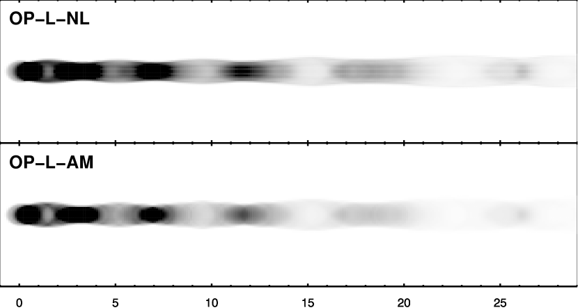
Figure 1.— Top panel: Synthetic (total intensity) radio map of the quiescent OP-L-NL model computed at an observational frequency of 43 GHz. Bottom panel: Same as top panel but for model OP-L-AM, and plotted using the same intensity scale. To compute the model OP-L-NL, 32 Lagrangian particles evenly distributed across the jet nozzle have been let to evolve. Since SPEV-NL does not include the effect of synchrotron losses on the NTP evolution, the differences between both radio maps are small. In both panels a $10^{\circ}$ jet viewing angle is assumed.

For the purpose of efficiently computing the synchrotron emissivity (see § 4), inside of each Lorentz factor bin $i$, we assume that, at any time, the number of NTPs per unit of energy and unit of volume $n^{0}_{i}(\tau,\gamma)$ ($\gamma_{i}(\tau)\leq\gamma<\gamma_{i+1}(\tau)$) follows a power-law and, therefore, the whole momentum distribution of NTPs consists of a piecewise power-law and,

$$n^{0}(\tau,\gamma)=n^{0}_{i}(\tau)\left(\frac{\gamma}{\gamma_{i}}\right)^{-q_{i}(\tau)},\>i=1,\dots,N_{\rm b},$$ (35)

where $n^{0}_{i}(\tau)$ is the number of particles with $\gamma=\gamma_{i}$ at the proper time $\tau$, and $q_{i}(\tau)$ is the power-law index of the distribution at the $i$-Lorentz factor interval. The values of $q_{i}(\tau)$ are computed numerically in every time step plugging Eq. (35) into Eq. (34) and solving iteratively the corresponding equation (which also involves knowing the interface values -Eq. (33)- and justifies why we need to follow the evolution of two sets of variables per bin).

The approach defined up to here has the advantage that, at every time level $\tau^{n}$, the momentum-space evolution and the physical space trajectory of the NTPs are decoupled during the corresponding time step $\Delta\tau$. The hydrodynamic evolution of the thermal plasma provides the values of $k_{\rm a}$ and $k_{\rm s}$ at the beginning of the time step ($\tau=\tau^{n}$), and once these values are known, it is possible to compute the momentum distribution of NTPs at time $\tau^{n+1}$. Thereby, it is possible to perform separately the trajectory integration of the NTPs once, and to evolve NTPs in the phase space afterward, as many times and with as many initial particle distributions as desired (viz., during a post-processing phase).

3.3. Normalization and initialization of the NTP distribution

Our models are set up such that we initially inject through the jet nozzle NTPs with a momentum distribution function which follows a single power-law, i.e., $q_{i}=q_{1},\forall i$. Therefore, the initial number and energy density in the interval $\gamma_{\rm min}\leq\gamma\leq\gamma_{\rm max}$ read

$${\cal N} = \frac{n^{0}_{1}}{q_{1}-1}\gamma_{\rm min}\left[1-\left(\frac{\gamma_{\rm max}}{\gamma_{\rm min}}\right)^{1-q_{1}}\right],$$ (36)

$${\cal U} = \frac{n^{0}_{1}}{q_{1}-2}\gamma_{\rm min}^{2}m_{\rm e}c^{2}\left[1-\left(\frac{\gamma_{\rm max}}{\gamma_{\rm min}}\right)^{2-q_{1}}\right]\,.$$ (37)

Consistent with our assumptions about the relation between the thermal and non-thermal populations we assume that ${\cal N}=c_{{}_{\cal N}}\rho/m_{\rm e}$ and ${\cal U}=c_{{}_{\cal U}}P$, where $c_{{}_{\cal N}}$ and $c_{{}_{\cal U}}$ are constants, while $P$ and $\rho$ stand for the pressure and rest-mass density of the background fluid, respectively. Such proportionalities along with Eqs. (36) and (37) yield (G95)

$$\gamma_{\rm min}=\frac{c_{{}_{\cal U}}}{c_{{}_{\cal N}}}\frac{q_{1}-2}{q_{1}-1}\frac{P}{\rho c^{2}}\frac{1-(\gamma_{\rm max}/\gamma_{\rm min})^{1-q_{1}}}{1-(\gamma_{\rm max}/\gamma_{\rm min})^{2-q_{1}}},$$ (38)

and we can use either Eq. (36) or Eq. (37) to compute $n^{0}_{1}$ if the ratio $C_{\gamma}:=\gamma_{\rm max}/\gamma_{\rm min}$ is fixed. Thus, the initial distribution of particles can be determined from pressure and rest-mass density at the jet nozzle, simply by specifying $c_{{}_{\cal N}}$ and $c_{{}_{\cal U}}$.

A key difference between SPEV and AM methods is that in SPEV the dimensionless proportionality parameters $c_{{}_{\cal N}}$ and $c_{{}_{\cal U}}$ are only specified at the jet injection nozzle. In the SPEV method, the subsequent time evolution of the NTP momentum distribution, namely, the spectral shape (piecewise power-law) and the limits of the distribution $\gamma_{\rm min}$ and $\gamma_{\rm max}$ as it evolves in the physical space is computed according to Eq. (28). AM ignores synchrotron loses, which yields a fixed power-law index for the whole distribution of Lorentz factors of the NTPs. The remaining two parameters needed to specify the distribution function, $\gamma_{\rm min}$ and $\gamma_{\rm max}$ are computed from the local values of the hydrodynamic variables. On the one hand, $\gamma_{\rm min}$ follows from Eq. (38) and $\gamma_{\rm max}$ is obtained from the fact that, $C_{\gamma}$ is strictly constant in time if the evolution is adiabatic. Also, in contrast to SPEV, it is necessary to assume a value of $C_{\gamma}$ everywhere in the simulated region and not only at the injection region.

4. Synchrotron radiation and synthetic radio maps

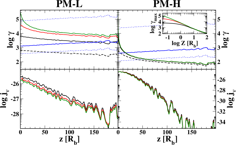
Figure 2.— Left and right panels correspond to quiescent models PM-L and PM-H, respectively. The upper panels display the spectral energy evolution along the jet axis. Thick black, red and green lines show the evolution of $\gamma_{\rm max}$ for initial values of $C_{\gamma}$ equal to $10$, $10^{2}$ and $10^{3}$, respectively. In the upper panels we overplot the values of the Lorentz factor corresponding to the maximum emission efficiency (solid blue line). The lower and upper $\gamma$ where the efficiency drops below 10% of the maximal as a function of distance for an observational frequency of 43 GHz are displayed by dotted blue lines above and below the maximum efficiency line, respectively. These blue lines have a positive slope since the magnetic field decreases with distance, so that ever larger Lorentz factors are needed to emit efficiently at a given frequency. The lower panels show the synchrotron emissivity of each model. The inset in the right panel shows the logarithm of $\gamma_{\rm max}$ as a function of the logarithm of $Z$ for the three models. It can be seen, that for the model PM-H, $\gamma_{\rm max}$ becomes virtually independent of its initial value at a distance larger than $\approx 1\,R_{b}$ from the jet nozzle. Please, note the difference in the scales of emissivity for the lower panels.

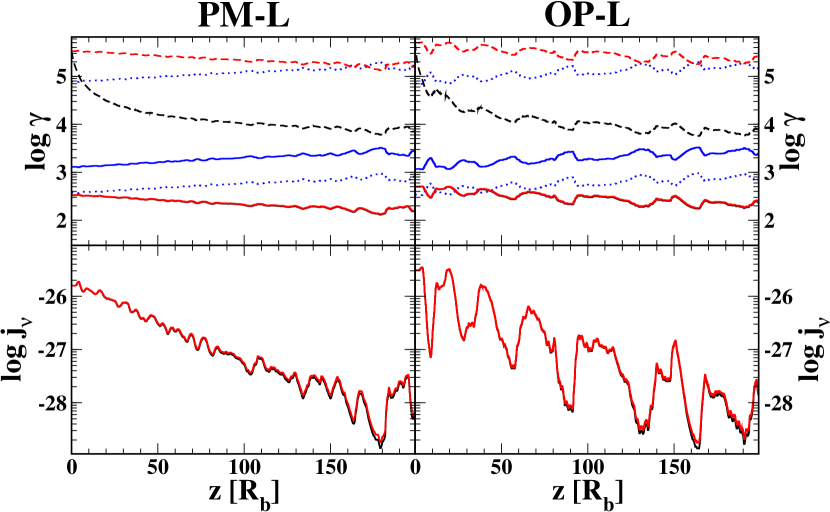
Figure 3.— In the whole figure, black (red) lines correspond to models computed with the SPEV (SPEV-NL) method. The left and right panels display properties of the PM-L and OP-L models, respectively. Upper panels: Spectral energy evolution along the jet axis for the stationary jet models. The values shown are computed in the jet comoving frame but the distance along the axis is measured in the laboratory frame (attached to the jet nozzle). The parameters of the spectral distribution of NTPs are the same as the ones of the reference model (§ 5). In the upper panel the thick lines track the values of $\gamma_{\rm min}$ (solid) and $\gamma_{\rm max}$ (dashed) of SPEV and SPEV-NL electron distributions as a function of the distance along the jet axis. Note that the lines corresponding to the values of $\gamma_{\rm min}$ for SPEV and SPEV-NL are almost indistinguishable. The curvature in the line corresponding to $\gamma_{\rm max}^{\rm SPEV}$, specially in the first $30R_{b}$, shows the effects of synchrotron cooling of the highest-energy SPEV particles. The blue lines have the same meaning as in Fig. 2. Lower panels: Synchrotron emissivity (Eq. 39) at the jet axis is shown as a function of the distance to the jet nozzle. For the parameters chosen, most of the electrons of both SPEV and SPEV-NL distributions emit synchrotron radiation efficiently in the whole jet. This makes that both, SPEV-NL and SPEV methods display a very similar emissivity dependence with distance along the jet axis (both curves are almost coincident).

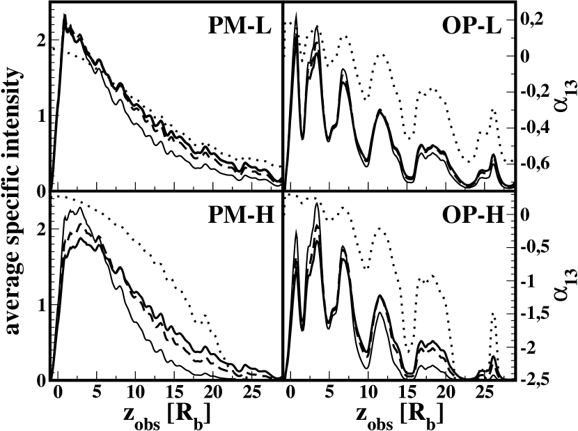
Figure 4.— Upper panels: Left and right panels display properties (as seen by a distant observer) of the PM-L and OP-L models, respectively, computed with the SPEV method. The thin-solid, dashed and thick solid lines correspond to the specific intensity at frequencies 43 GHz, 22 GHz and 15 GHz respectively. The intensities are obtained directly from the models without convolving the data. For clarity, all the specific intensities are normalized to a common value. The dotted line shows the spectral index $\alpha_{13}$. Lower panels: Same as the upper panels, but for the models PM-H and OP-H.

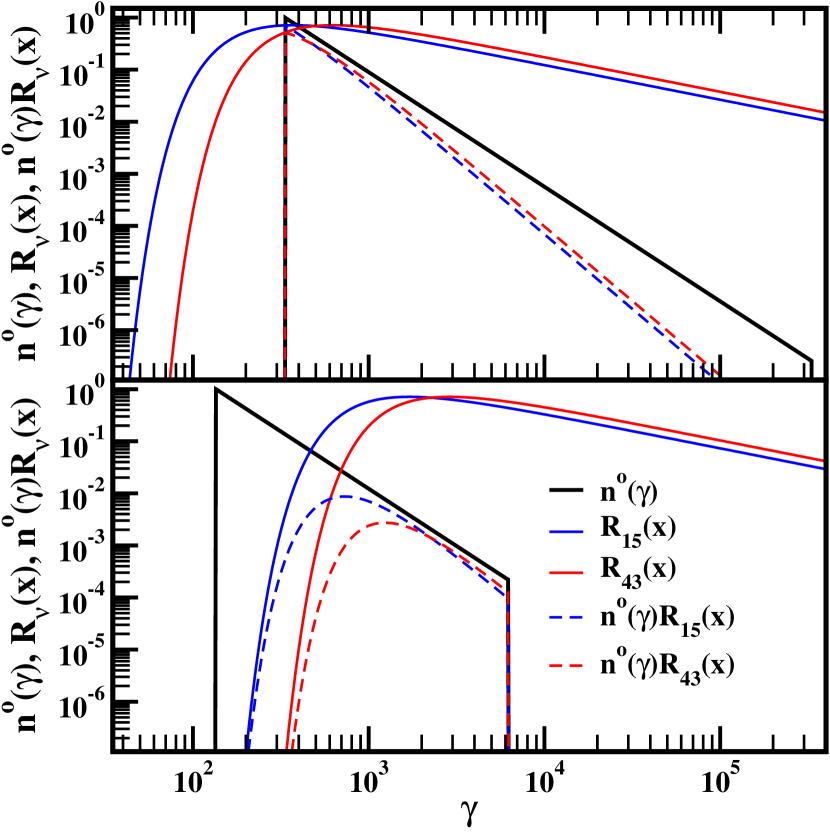
Figure 5.— The number of particles per unit of energy and unit of volume $n^{0}(\gamma)$ is displayed with a solid black line as a function of $\gamma$ for the PM-L model. We omit the temporal dependence of $n^{0}(\tau,\gamma)$ in Eq. (35) because we are considering quiescent jet models. The solid blue and red lines show the synchrotron function $R_{\nu}(x)$ (Eq. 41) at frequencies 15 GHz and 43 GHz, respectively, while the products $n^{0}(\gamma)R_{15}(x)$ and $n^{0}(\gamma)R_{43}(x)$ are displayed with dashed blue and red lines, respectively. The later products are precisely the integrand of the synchrotron emissivity (Eq. 39). Lower panel: Corresponds to the typical conditions one encounters downstream the jet ($\gamma_{\rm min}\sim 135$, $\gamma_{\rm max}\sim 6\times 10^{3}$, $b\sim 0.002$ G). Upper panel: Corresponds to the conditions found close to the injection nozzle ($\gamma_{\rm min}=330$, $\gamma_{\rm max}=3.3\times 10^{5}$, $b_{b}\sim 0.02$ G).

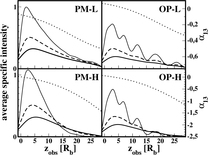
Figure 6.— Same as Fig. 4, but in this case the specific intensities are obtained by convolving the data with a circular Gaussian beam whose radius at FWHM are $2.25R_{b}$, $4.40R_{b}$ and $6.45R_{b}$ at frequencies 43 GHz, 22 GHz and 15 GHz, respectively. With this convolution we degrade the resolution of our data to limits comparable with VLBI observations.

The synchrotron emissivity, at a time $\tau$, of an ensemble of NTPs advected by a thermal plasma element, can be cast in the following general form (valid both for ordered and random magnetic fields; see Mimica, 2004)

$$j(\tau,\nu)=\frac{\sqrt{3}e^{3}b_{\perp}}{4\pi m_{\rm e}c^{2}}\sum_{i=1}^{N_{\rm b}}\int_{\gamma_{i}(\tau)}^{\gamma_{i+1}(\tau)}{\mathrm{d}}\gamma n^{0}(\tau,\gamma)g\left(\frac{\nu}{\nu_{\perp}\gamma^{2}}\right)\,,$$ (39)

where $(g(x),b_{\perp},\nu_{\perp})=(R(x),|{\bf b}|,\nu_{0})$ if ${\bf b}$ is randomly oriented, or $(g(x),b_{\perp},\nu_{\perp})=(F(x),|{\bf b}|\sin\alpha,\nu_{0}\sin\alpha)$ in case ${\bf b}$ is ordered. $\alpha$ is the angle the comoving magnetic field forms with the line of sight, and $\nu_{0}=3e|{\bf b}|/4\pi m_{\rm e}c$. In the previous expressions, $F$ is the first synchrotron function

$$F(x)=x\int_{x}^{\infty}d\xi K_{5/3}(\xi),$$ (40)

$K_{5/3}$ being the modified Bessel function of index $5/3$, and $R$ is defined as

$$R(x):=\frac{1}{2}\int_{0}^{\pi}{\mathrm{d}}\alpha\sin^{2}\alpha\ \ F\left(\frac{x}{\sin\alpha}\right)\,.$$ (41)

The synchrotron self-absorption process is also included in our algorithm. Thus, we need to compute the synchrotron absorption coefficient, at a time $\tau$, of an ensemble of NTPs advected by a thermal plasma element, which can be cast in the following general form

$$\kappa(\tau,\nu) = \frac{\sqrt{3}e^{3}b_{\perp}}{8\pi m_{\rm e}^{2}c^{2}\nu^{2}}\times$$

$$\sum_{i=1}^{N_{\rm b}}\int_{\gamma_{i}(\tau)}^{\gamma_{i+1}(\tau)}{\mathrm{d}}\gamma\left[-\gamma^{2}\frac{{\mathrm{d}}}{{\mathrm{d}}\gamma}\left(\frac{n^{0}(\tau,\gamma)}{\gamma^{2}}\right)\right]g\left(\frac{\nu}{\nu_{\perp}\gamma^{2}}\right)\,,$$

In order to perform the integrals of Eq. (39) and (4), it is necessary to make some assumption about the internal distribution of NTPs within each Lorentz factor bin $i$. As explained in Sect. 3.2, we choose to assume that NTPs distribute as power-law (Eq. 35) inside of each bin. This choice agrees with the common assumptions made in the literature and is also supported by theoretical arguments and observations of discrete radio sources (e.g., Pacholczyk, 1970, chapt. 6; Königl, 1981), and by numerical simulations (e.g., Achterberg, et al., 2001). Furthermore, it allows us to build a very efficient and robust method for computing the local synchrotron emissivity and the local absorption coefficient. It consist of tabulating the functions $F(x)$ and $R(x)$, and then tabulating integrals over power-law distributions of particles. Proceeding in this way is $\sim 100$ times faster than computing Eqs. (39)-(41) by direct numerical integration.

The synchrotron coefficients (Eqs. 39 and 4) of steady jet models result from the time evolution of the Lagrangian particles injected at the jet nozzle and spatially transported along the whole jet (the larger the number of Lagrangian particles, the better coverage of the whole jet). In our simulations around $N_{\rm steady}=32$ of such Lagrangian particles (i.e., about 4 particles per numerical cell at the injection nozzle) are sufficient to properly cover a quiescent jet. If the jet is not steady, e.g., because a hydrodynamic perturbation is injected, we need to follow many more Lagrangian particles. It becomes necessary to have particles everywhere the quiescent jet is perturbed. For the models in this paper, this means to inject new Lagrangian particles through the jet nozzle at all time steps after a hydrodynamic perturbation is set in. The distribution function of the NTPs injected with the perturbation is the same as that of the particles injected in the quiescent jet. This is justified since the perturbation only changes the bulk Lorentz factor, but not the pressure, or the density of the fluid. In the simulations where we have injected a hydrodynamic perturbation this implies that we must follow the evolution of more than $N_{\rm steady}\times N_{\rm timesteps}\mathrel{\hbox to0.0pt{\lower 4.0pt\hbox{\hskip 1.0pt$\sim$}\hss}\raise 1.0pt\hbox{$>$}}10^{5}$ Lagrangian particles. This makes our SPEV simulations effectively four-dimensional (two spatial, one momentum and a -huge- number of Lagrangian particles dimension). Therefore, the spatial resolution that we may afford results severely limited.

The synchrotron coefficients depend on the magnetic field strength and orientation as well as on the spectral energy distribution $n^{0}(\tau,\gamma)$. In our models the magnetic field is dynamically negligible, thus we set it up ad hoc. We choose that $U_{\rm B}$ remains a fixed fraction of the particle energy density and that the field is randomly oriented.

Synthetic radio maps are build by integrating the transfer equations for synchrotron radiation along rays parallel to the line, accounting for the appropriate relativistic effects (time dilation, Doppler boosting, etc.). The technical details relevant for this procedure can be found in Appendix A.

5. Radio emission

The goals of this section are twofold. First, we validate the new algorithm comparing the synthetic radio maps obtained with SPEV without accounting for synchrotron losses with the ones obtained using AM. For this purpose, we will employ the SPEV method to evolve NTPs but taking $k_{\rm s}=0$ in Eq. (25). We will refer to this method of evaluating the evolution of NTPs as SPEV-NL. Second, we will show the differences induced by accounting for synchrotron losses in the evolution of NTPs.

5.1. Calibration of the method

In order to properly compare SPEV-NL and AM results we set up the same spectral parameters at the jet nozzle for both: $q_{1}=2.2$, $\gamma_{\rm min}=330$, $C_{\gamma}=10^{3}$ and $\rho_{a}=2\times 10^{-21}\,$g cm^-3. We produce all our images for a canonical viewing angle of $10^{\circ}$ and assuming that $R_{b}=0.1\,$pc. The comoving magnetic field strength is ${\rm b}_{b}:=\sqrt{{\bf b}^{2}}=0.02\,$G (model PM-L-NL) and 0.03 G (model OP-L-NL).

For the set of reference parameters we have considered, the synthetic radio maps of the quiescent jets produced with SPEV-NL yield very small differences with respect those computed with AM (Fig. 1). Indeed, the overall agreement between both methods in the predicted quiescent radio maps is remarkably good, particularly, if we consider the fact that SPEV is a Lagrangian method while AM is Eulerian.

Looking at the synthetic radio maps of model OP-L-NL (Fig. 1), we observe, as in G97, a regular pattern of knots of high emission, associated with the increased specific internal energy and rest-mass density of internal oblique shocks produced by the initial overpressure in this model. The intensity of the knots decreases along the jet due to the expansion resulting from the gradient in external pressure. Some authors (e.g., Daly & Marscher 1988; G95; G97; Marscher, et al. 2008) propose that the VLBI cores may actually correspond to the first of such recollimation shocks. Since, for the parameters we use, the source absorption for frequencies above 1 GHz is negligible, the jet core reflects the ad hoc jet inlet in the PM-L-NL model, while we shall associate it with the first recollimation shock for model OP-L-NL. The rest of the knots are standing features in the radio maps for which, there exists robust observational confirmation (Gómez, 2002, 2005).

Since the synchrotron losses affect more the higher energy part of the distribution of NTPs than the lower one, we have also validated our code by considering the dependence of the results with the limit $\gamma_{\rm max}$ and checked them against the theoretical expectations (e.g., Pacholczyk, 1970). For this we reduce the value of $\gamma_{\rm max}$ keeping all other parameters fixed and equal to those of the PM-L model. Since the value of $\gamma_{\rm max}$ is set by the ratio $C_{\gamma}$, in order to study the dependence of the results with $\gamma_{\rm max}$, we have computed a set of models combining three different values of $C_{\gamma}=\{10^{3},10^{2},10\}$ and ${\rm b}_{b}=0.02$ G. Additionally, to highlight the effect of the radiative losses, we have performed the same simulations (varying $C_{\gamma}$) for a larger value of the beam magnetic field, equal to that of the model PM-H.

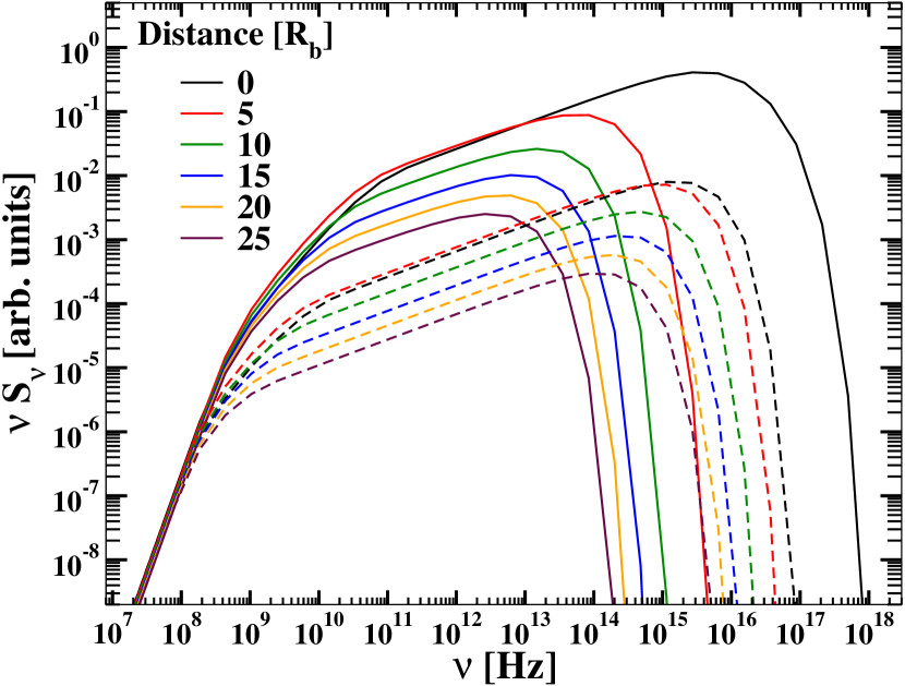
Figure 7.— The different lines in the plot show the spectral energy distribution of selected points along the jet axis of model PM with two different magnetic fields. All the models have been computed using the SPEV method with the reference parameters of § 5. Solid lines correspond to the PM-L model and dashed lines to the PM-S model. The distance to the nozzle (in $R_{b}$) to which each spectrum corresponds is provided in the legend. Synchrotron self-absorption is dominant at frequencies below few hundred MHz.

Figure 8.— Same as Fig. 1, but in this case for the OP-H model.

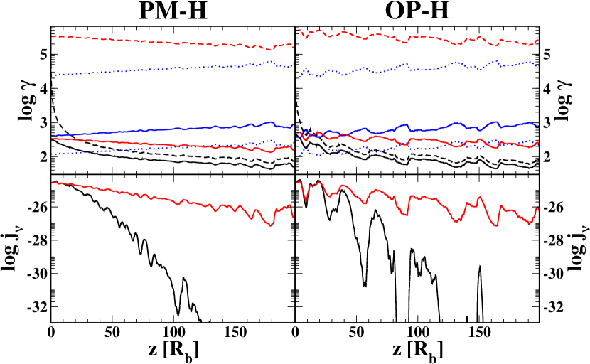
Figure 9.— Same as Fig. 3 but for the PM-H and OP-H models. In this case, the synchrotron losses in SPEV are so important that, $\gamma_{\rm max}^{\rm SPEV}$ leaves the efficient synchrotron radiation regime. The point where this happens depends on the model. The crossing of the $\gamma_{\rm max}^{\rm SPEV}$ with the line denoting a 10% synchrotron efficiency limit occurs when the particles reach $z\sim 50R_{b}$ for model PM-H and much earlier $z\sim 24R_{b}$ in case of model OP-H. After this line crossings the whole distribution radiates very little at the considered observational frequency. This produces a substantial dimming of SPEV models at large $z$. The difference in the emissivity as a function of the distance $z$ is larger for the PM-H model than for the OP-H model because of the re-compressions that the SPEV-NTP experiences at shocks.

For model PM-L (Fig. 2, left panel), radiative losses are negligible, and the reduction in $C_{\gamma}$ (i.e., in $\gamma_{\rm max}$), does not change appreciably the radio maps at radio observing frequencies. Indeed, except the model with the lowest $C_{\gamma}$ (corresponding to $\gamma_{\rm max}=2200$) beyond $160\,R_{b}$, all the models stay above the 100% efficient radiation limit along the whole jet.

The models with larger magnetic field ${\rm b}_{b}=0.2\,$G (Fig. 2, right panel), undergo a much faster evolution. The emissivity along the jet axis drops very quickly and at $z=150R_{b}$, it is five orders of magnitude smaller than for the PM-L model. After a very short distance ($\simeq 1\,R_{b}$), synchrotron losses bring $\gamma_{\rm max}$ of all three models to a common value which is independent of the initial one (note that the variation of $\gamma_{\rm max}$ with distance is indistinguishable for the three models except in the zoom displayed in the inset of the top right panel of Fig. 2). The reason for this degenerate evolution resides in the relatively large magnetic field strength (see Pacholczyk, 1970, Eq. 6.20). Thus, our method is able to reproduce the common evolution of models with different values of $\gamma_{\rm max}$ and a relatively large magnetic field.

5.2. On the relevance of synchrotron losses

Having verified that our method (SPEV-NL) compares adequately to the AM, we now turn to the specific role that synchrotron losses play in the evolution of NTPs. For that, we compare in Fig. 3 the spectral properties of NTPs in quiescent jet models using both SPEV-NL and SPEV methods. It is obvious that the highest energy particles of the distribution cool down rather quickly (see the fast decay of the dashed black curves in the upper panels of Fig. 3) even for the small value of ${\rm b}_{b}$ considered here. Most of the spectral evolution triggered by synchrotron cooling at high values of $\gamma$ happens in the first $25R_{b}-50R_{b}$. After that location, the ratio $C_{\gamma}$ is much smaller than at the injection nozzle ($C_{\gamma}\mathrel{\hbox to0.0pt{\lower 4.0pt\hbox{\hskip 1.0pt$\sim$}\hss}\raise 1.0pt\hbox{$<$}}50$), and the evolution of the NTP population is dominated by the adiabatic cooling/compression downstream the jet. In contrast, the upper limit of the SPEV-NL distribution (dashed red curves in the upper panels of Fig. 3) only changes by a factor of 2 along the whole jet length. Theoretically, it is well understood that it is possible to undergo a substantial spectral evolution (triggered by synchrotron losses) and, simultaneously, not to have any manifestation of such evolution at radio frequencies (e.g., Pacholczyk, 1970). The substantial decrease of $\gamma_{\rm max}$ triggered by the radiative losses, does not affect much the value of the integral that has to be performed over $\gamma$ in order to compute the emissivity in Eq. (39), since most of the emitted power at radio-frequencies happens relatively close to $\gamma_{\rm min}$, where synchrotron losses are negligible. Certainly, at higher observing frequencies this is not the case, and the emissivity substantially drops because of the fact that both, the synchrotron losses (Eq. 18) and the frequency at which the spectral maximum emission is reached depend on the square of the non-thermal electron energy (and on the magnetic field strength).

We define the spectral index between two radio frequencies as

$$\alpha_{ij}=\frac{\log{(S_{i}/S_{j})}}{\log{(\nu_{i}/\nu_{j})}},$$ (43)

where $S_{i}$ and $S_{j}$ are the flux densities at the frequencies $\nu_{i}$ and $\nu_{j}$, respectively. Since we compute synthetic radio maps at three different radio frequencies ($\nu_{1}=15\,$GHz, $\nu_{2}=22\,$GHz, and $\nu_{3}=43\,$GHz), we may define three different spectral indices. For convenience, in the following, we consider the spectral index $\alpha_{13}$ between 15 GHz and 43 GHz. Furthermore, we may compute $\alpha_{13}$ for both convolved or unconvolved flux densities. The unconvolved flux density is directly obtained from the simulations and has an extremely good spatial resolution, viz. the unconvolved radio images have a resolution comparable to that of the hydrodynamic data. The convolved flux densities result from the convolution with a circular Gaussian beam of the unconvolved data. The FWHM of the Gaussian beam is proportional to the observing wavelength. This convolution is necessary to degrade the resolution of our models down to limits comparable with typical VLBI observing resolution. We note that in order to compute the spectral index for convolved flux densities, we have to employ the same FWHM convolution kernel for the data at the two frequencies under consideration. Thus, to compute $\alpha_{13}$ for convolved data, we employ the same Gaussian beam with a FWHM 6.45 $R_{b}$ for both flux densities at 15 GHz and 43 GHz.

Our models are computed for an electron spectral index $q=q_{1}=2.2$. We verify that, at large distances to the jet nozzle, unconvolved models (Fig. 4 upper panels) tend to reach the expected value $\alpha=(1-q)/2=-0.6$ for an optically thin source. This asymptotic value is reached smoothly in case of the PM-L and PM-H models and it is modulated by the presence of inhomogeneities (recollimation shocks) in the beam of models OP-L and OP-H.

Close to the jet nozzle, our unconvolved models display flat or even inverted ($\alpha_{13}>0$) spectra (Fig. 4), in spite of the fact that the jets are optically thin throughout their whole volume. The occurrence of flat or inverted spectrum depends on the magnetic field strength and differs for OP and PM models. As shown in Fig. 4, the PM-L model shows an inverted spectrum for $z\mathrel{\hbox to0.0pt{\lower 4.0pt\hbox{\hskip 1.0pt$\sim$}\hss}\raise 1.0pt\hbox{$<$}}2.5R_{b}$, while the OP-L model displays a pattern of alternated inverted and normal ($\alpha_{13}<0$) spectra for $z\mathrel{\hbox to0.0pt{\lower 4.0pt\hbox{\hskip 1.0pt$\sim$}\hss}\raise 1.0pt\hbox{$<$}}12.5R_{b}$. The spectral inversion in the OP-L model happens where standing features (associated to recollimation shocks in the beam) are seen in the jet.

If synchrotron losses are not included, the spectral behavior of models PM-L and OP-L remains unchanged, because in such a case loses are negligible. However, if for the models PM-H and OP-H the losses are not accounted for (which is, obviously, a wrong assumption), the jet displays an inverted spectrum up to distances $z\sim 30R_{b}$.

The behavior of the spectral index exhibited by our models close to the jet nozzle contrasts with the theoretical expectations for an inhomogeneous, optically thin jet with a negative electron spectral index, for which the jet inhomogeneity is predicted to steepen the spectrum (e.g., Marscher, 1980; Königl, 1981). To explain this discrepancy we argue that the analytic predictions are based on the assumption that the limits of the energy distribution of the NTPs safely yield that the contribution of the synchrotron functions (Eqs. 40 and 41) to the synchrotron coefficients (Eqs. 39 and 4) is proportional to some power of the frequency and of the NTP’s Lorentz factor. This situation does not happen if the lower limit of the distribution $n^{0}(\gamma)$, $\gamma_{\rm min}$, is (roughly) larger than the value $\gamma_{{}_{\rm M}}$ at which the synchrotron function $R(x_{\rm low})$ (Eq. 41) reaches its maximum, where $x_{\rm low}=\nu_{\rm low}/\nu_{0}\gamma^{2}$, and $\nu_{\rm low}$ is the smallest observing frequency in the comoving frame. Since the function $R(x)$ has a maximum for $x\simeq 0.28$, one finds that the condition to have an inverted spectrum is $\gamma_{\rm min}\mathrel{\hbox to0.0pt{\lower 4.0pt\hbox{\hskip 1.0pt$\sim$}\hss}\raise 1.0pt\hbox{$>$}}\gamma_{{}_{\rm M}}\simeq 1.9\times(\nu_{\rm low}/\nu_{0})^{1/2}{\cal D}^{-1/2}$, where ${\cal D}:=1/\Gamma(1-v\cos{\theta})$ is the Doppler factor. Since, in our case, $\nu_{\rm low}=15$ GHz, we may also write

$$\gamma_{\rm min}\mathrel{\hbox to0.0pt{\lower 4.0pt\hbox{\hskip 1.0pt$\sim$}\hss}\raise 1.0pt\hbox{$>$}}113\left(\frac{\nu_{\rm low}}{\rm 15\,GHz}\right)^{1/2}\left(\frac{b}{\rm 1\,G}\right)^{-1/2}{\cal D}^{-1/2}.$$ (44)

Figure 5 shows how this boundary effect substantially modifies the emissivity at 15 GHz and 43 GHz for the model PM-L. At the injection nozzle (Fig. 5 upper panel) the lower limit of the integral in Eq. (39) is set by $\gamma_{\rm min}$ and not by the lower limit of $R_{\nu}(x)$. However, downstream the jet (Fig. 5 lower panel) the situation reverses and the fast decay of $R_{\nu}(x)$ for $\gamma<300$ sets the lower limit of the emissivity integral. Thus, close to the nozzle, the value of the area below the $n^{0}(\gamma)R_{43}(x)$ curve, which is proportional to the emissivity at 43 GHz, is larger than that below the curve $n^{0}(\gamma)R_{15}(x)$. Hence, there is an emissivity excess at 43 GHz compared to that at 15 GHz. As a result, the $\alpha_{13}$ becomes positive close to the jet nozzle. Far away from the nozzle the emissivity at 15 GHz almost doubles that at 43 GHz, explaining why values of $\alpha_{13}<0$ are reached asymptotically.

The convolved models display some traces of the behavior shown for the uncovolved ones. For example, OP models display a flat or inverted spectrum very close to the jet nozzle (Fig. 6 right panels). This is not the case for PM-L model (Fig. 6). Since the resolution of the convolved data is much poorer than that of the unconvolved one, $\alpha_{13}$ exhibits a quasi monotonically decreasing profile from the jet nozzle (where $-0.1\mathrel{\hbox to0.0pt{\lower 4.0pt\hbox{\hskip 1.0pt$\sim$}\hss}\raise 1.0pt\hbox{$<$}}\alpha_{13}\mathrel{\hbox to0.0pt{\lower 4.0pt\hbox{\hskip 1.0pt$\sim$}\hss}\raise 1.0pt\hbox{$<$}}0$). The coarse resolution of the convolved data also blurs any signature in the spectral index associated to the existence of cross shocks in the beam of OP models. Furthermore, the decay with distance of the spectral index is shallower for the convolved flux data than for the unconvolved one. Hence, the theoretical value $\alpha_{13}=-0.6$, which is expected for an optically thin synchrotron source, is reached nowhere in the jet models PM-L and OP-L (Fig. 6).

As expected, at frequencies below a few hundred MHz, the jet is strongly self-absorbed everywhere (Fig. 7). Close to the jet nozzle, there is not a clear turnover frequency between the self-absorbed part of the spectrum and the optically thin one. Instead, we observe a smooth transition between both regimes. Far from the nozzle, the self-absorption turnover is much more peaked. It is known (Tsang & Kirk, 2007) that in contrast with a distribution of NTP that follows a power-law extending to $\gamma_{\rm min}\mathrel{\hbox to0.0pt{\lower 4.0pt\hbox{\hskip 1.0pt$\sim$}\hss}\raise 1.0pt\hbox{$>$}}1$, if the power-law is restricted to a relatively large, but not unrealistic $\gamma_{\rm min}$, or if the electron distribution was monoenergetic, the intensity can be flat over nearly two decades in frequency (which implies that the energy flux grows linearly over the same frequency range). Our PM-L models have $\gamma_{\rm min}=330$ at the injection nozzle and reduce it to $\gamma_{\rm min}\simeq 200$ at $z=200R_{b}$ because of the adiabatic expansion of the jet (Fig. 3 upper left). As we have argued in § 5 close to the jet nozzle, $\gamma_{\rm min}\mathrel{\hbox to0.0pt{\lower 4.0pt\hbox{\hskip 1.0pt$\sim$}\hss}\raise 1.0pt\hbox{$>$}}\gamma_{{}_{\rm M}}$, which means that $\gamma_{\rm min}$ is sufficiently large to be in the range where a smooth turnover transition is expected, in agreement with Tsang & Kirk (2007). Far away from the nozzle, since $\gamma_{\rm min}$ decreases, we recover the more standard situation in which an obvious turnover frequency can be identified.

Provided that close to the nozzle our PM (also OP) models are weakly self-absorbed (at 15 GHz, the solid black line in Fig. 7 has not reached the power-law regime yet), one may question whether the spectral inversion we have found is not also the result of opacity effects. We have dismissed such a possibility by running models with the SPEV method including no absorption.

5.2.1 Dependence with the magnetic field strength

In order to study the effect of intense synchrotron losses we consider models PM-H and OP-H (Figs. 8 and 9). Very close to the injection nozzle ($Z\sim 50\,R_{b}$) the line denoting the evolution of $\gamma_{\rm max}^{\rm SPEV}$ crosses the line corresponding to a 10% synchrotron efficiency limit (lower blue thick line; Fig. 9) and most of the synchrotron emissivity falls outside of the observational frequency. Because of a stronger magnetic field than in models PM-L and OP-L, more energy is lost close to the jet nozzle than far from it and, thus, SPEV-radio-maps look much shorter than SPEV-NL-radio-maps (Fig. 8). An alternative way to see such an effect is through the rapid decay of $\gamma_{\rm max}^{\rm SPEV}$ in the first $10R_{b}$ in Fig. 9, right panel. Afterwards, the adiabatic changes dominate the NTP evolution. The initial period of fast evolution is even shorter if a larger magnetic field were to be considered.

The intensity contrast between shocked and unshocked jet regions of model OP-H (Fig. 9) is larger than that of model OP-H-NL. Indeed, the OP-H model appears as a discontinuous jet (Fig. 8) because of the slightly larger intensity increase than in the OP-H-NL model when the NTP distribution passes through cross-shocks and the much more pronounced intensity decrease at rarefactions. We note that, although the adiabatic evolution is followed with the same algorithm in SPEV and SPEV-NL, the radiative losses change substantially the NTP distribution that it is injected through the nozzle after very short distances. The consequence being that the NTP distribution $n^{0}(\tau,\gamma)$ that faces shocks and rarefactions downstream the nozzle is rather different when using SPEV or SPEV-NL method and, therefore, the relative intensity of shocked and unshocked regions is also different depending on whether synchrotron losses are included or not in the calculation.

The outlined differences between models OP-H and OP-H-NL (with shocks in the beam), have to be interpreted with caution since none of the methods accounts for the injection of high-energy particles at shocks. But independent of this, we expect that if the magnetic field is sufficiently large, the SPEV method will yield a rather fast evolution of such particles and, thereby, a faster decay of the intensity downstream the shock.

The most relevant difference between the upper and lower panels of Fig. 8, is the increased brightness of the jet close to the injection nozzle and the steeper fading of the jet when energy losses are included. This fact poses the paradox that the method that accounts for radiative losses (SPEV) yields brighter standing features close to the injection nozzle (far from the nozzle the situation reverses and the SPEV-NL model is brighter than SPEV one). In order to disentangle this apparent contradiction, we shall consider that the plasma is compressed at standing shocks, which yields a growth of the magnetic field energy density (proportional to the pressure in our case), and triggers a faster cooling of the high-energy particles. Since the SPEV method conserves the number density of NTPs (Eq. 36), due to the synchrotron losses, high-energy particles reduce their energy and accumulate into an interval of Lorentz factor which is smaller than in the case of SPEV-NL models. As in such reduced Lorentz factor interval NTPs radiate more efficiently at the considered radio-frequencies, the emissivity of SPEV models at strong compressions (like, e.g., the considered cross shocks) becomes larger than that corresponding to models which do not include synchrotron losses. It is important to note that this situation happens in our models rather close to the jet nozzle. The reason being that after the NTPs have suffered a substantial synchrotron cooling, the evolution of the NTP distribution is dominated by the adiabatic terms of Eq. 25. In such a regime, reached by our models at a certain distance from the jet nozzle, the evolution of SPEV-NL and SPEV models is qualitatively similar. Considering the different qualitative evolution of the NTP distribution close to the nozzle and far from it, we refer to such epochs as losses-dominated and adiabatic regimes, respectively. These terms agree with the commonly used in the literature to refer to similar phenomenologies (e.g., Marscher & Gear 1985).

For PM-H and OP-H models, the spectral behavior is dominated by the change of slope of the NTP Lorentz factor distribution beyond the synchrotron cooling break at $\gamma=\gamma_{\rm br}$. Theoretically, an optically thin inhomogeneous jet shall display a spectral index $\alpha=(q+1)/2$, if the radiation in the observational band is dominated by the electrons with Lorentz factors $\gamma\mathrel{\hbox to0.0pt{\lower 4.0pt\hbox{\hskip 1.0pt$\sim$}\hss}\raise 1.0pt\hbox{$>$}}\gamma_{\rm br}$, or $\alpha\simeq-2.7$ if the emission is dominated by electrons with Lorentz factors close to $\gamma_{\rm max}$ (Königl, 1981). Figure 4 (lower panels) shows that asymptotically (viz., at large $z$) unconvolved models reach values $\alpha_{13}\mathrel{\hbox to0.0pt{\lower 4.0pt\hbox{\hskip 1.0pt$\sim$}\hss}\raise 1.0pt\hbox{$<$}}-2.5$, implying that the highest energy electrons with $\gamma\sim\gamma_{\rm max}$ are the most efficiently radiating at the considered observing frequencies. The value of $\gamma_{\rm max}$ differs significantly when synchrotron loses are not included. This fact explains the inversion of the spectrum along the whole jet if synchrotron losses were not included (PM-H-NL and OP-H-NL models). Thereby, synchrotron losses tend to produce a “normal” spectrum ($\alpha_{ij}<0$) if the magnetic field is large.

Regarding the convolved data, we note that models with a higher magnetic field display the same qualitative phenomenology discussed in § 5. In this case, the theoretical value $\alpha\simeq-2.7$ is not reached neither by the PM-H ($\alpha_{13,min}^{\rm PM-H}=-1.4$) nor by the OP-H ($\alpha_{13,min}^{\rm OP-H}=-1.1$) model (Fig. 6 lower panels).

6. Infrared to X-rays emission

We have computed the spectral properties of some of our quiescent jet models above radio frequencies. We note, that we have not included any particle acceleration process at shocks in the SPEV method, thus, the spectrum beyond infrared frequencies has to be taken carefully. If any shock acceleration mechanism were included, a larger contribution of the shocked regions will be present. In addition, the inverse Compton process, may shape the emission at such high energies, and such cooling process is presently not included in SPEV.

The results for models PM-S and PM-L (Tab. 1), which have no or extremely weak shocks are displayed in Fig. 7, where we show the spectral energy distribution at selected distances from the nozzle for points located along the jet axis. The small magnetic field of model PM-S (Fig. 7 dashed lines) minimizes the energy losses, but also the observed flux in the optical or X-ray band, rendering observable at such wavelengths the hydrodynamic jet models considered here (if the jet is sufficiently close). In the case of model PM-L, right at the nozzle ($z=0$ in Fig. 7), the energy flux cut-off is located at $\simeq 10^{18}\,$Hz. This means that, we could observe the jet core in the soft X-ray band, if the source was sufficiently close. However, the core size at such frequencies is very small (as it is expected; see e.g., Marscher & Gear 1985). This is reproduced in our models since at such a short distance as $z=5R_{b}$, the jet can barely be observed in the Near Ultraviolet or, perhaps in the optical band (Fig. 7, red solid line), but there is virtually no flux in the X-ray band because of the fast NTP cooling for the considered magnetic field energy density at the jet nozzle. In the Near Infrared range, the jet could perhaps be observable up to distances of $10R_{b}-15R_{b}$. A larger magnetic field drives a faster cooling, rendering undetectable the jet even at infrared frequencies. This phenomenology has been invoked to explain the relative paucity of optical jets with respect to radio jets. However, there are a number of authors which claim that a large proportion of jets generate significant levels of both optical and, even, X-ray emission (e.g., Perlman, et al., 2006). Our results shall not be taken in support of any of the two thesis since energy losses depend also on the magnetic field strength (Eq. 18), which we fix ad hoc.

7. Evolution of a superluminal component

In this section we discuss the time dependent observed emission once a hydrodynamic perturbation is injected into the jet (see Sec. 2.1). Following the convention of G97, we call components to local increases of the specific intensity in a radio map, while we use perturbation to denominate the variation of the hydrodynamic conditions injected through the jet nozzle. In order to magnify the effect of synchrotron losses in our models, we discuss models PM-H and OP-H in Sec. 7.1, and we also look for the differences between the PM and OP models. While the standing shocks of the beam of model OP-H are very weak, the shocks developed by the hydrodynamic perturbation are rather strong. Since we have not included in our method the acceleration of NTPs at relativistic shocks, computing the synchrotron emission at frequencies above radio may yield inconsistent results. Therefore, we only analyze the spectral properties of the emission in radio bands. Finally we show spacetime plots of hydrodynamic and emission properties along the jet axis in Sec. 7.2.

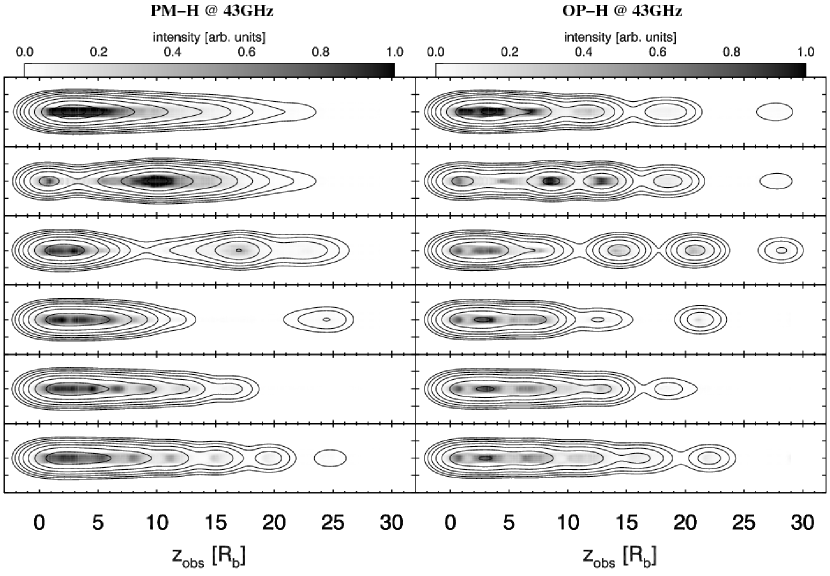
Figure 10.— Snapshots of the emission at 43 GHz due to component evolution computed with the SPEV method, for the PM-H (left) and OP-H (right) models. From top to bottom panels show the observed emission $0.02$, $0.39$, $0.75$, $1.12$, $1.94$ and $4.58$ years after the component appears. The same gray scale has been used for all snapshots. The superimposed contours have been obtained by convolving the image with a circular Gaussian beam whose radius at FWHM is $2.25R_{b}$. The contour levels are 0.005, 0.01, 0.02, 0.04, 0.08, 0.16, 0.32, 0.64 and 0.9 of the maximum of the convolved emission. The horizontal length scale is expressed in units of $R_{b}=0.1\,$pc, while the vertical length scale has been compressed and spans only $10R_{b}$. The main component has moved out of the right boundary in the lower two panels.

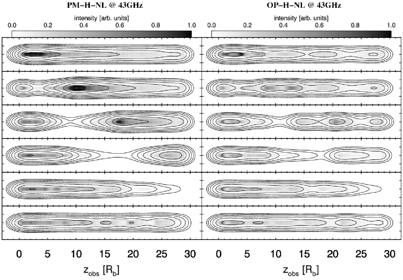
Figure 11.— Same as Fig. 10, but without including synchrotron losses (SPEV-NL method).

7.1. On the relevance of synchrotron losses

The magnetic field energy density is set ad hoc in our models (Sect. 4), and we can change it freely if the resulting magnetic field does not become dynamically relevant.

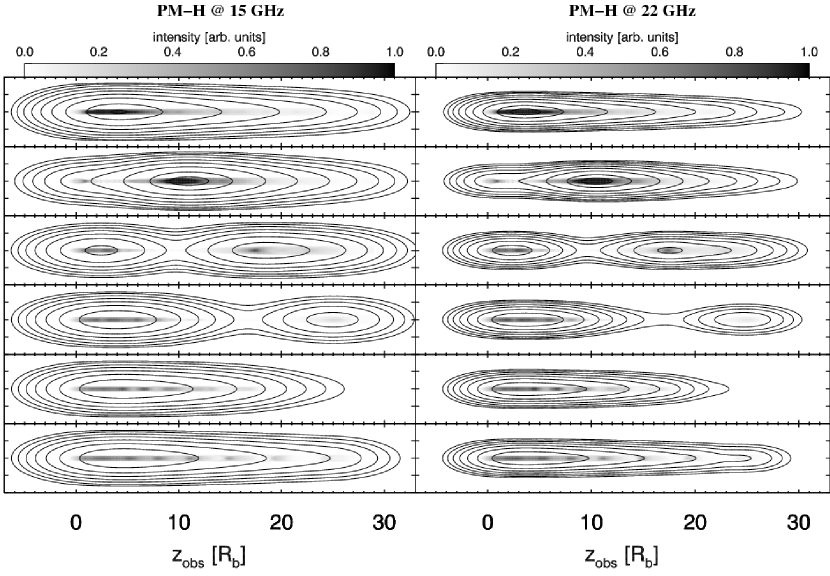
Figure 12.— Same as Fig. 10, but only showing the PM-H model observed at 15 GHz (left) and 22 GHz (right). The images at each frequency use an intensity gray scale separately normalized to the maximum at the corresponding frequency. The vertical scale spans $20R_{b}$, i.e., there is a factor of two difference between the vertical scales shown in Fig. 10 and in this figure. Since the FWHM of the convolution beam depends linearly on the wavelength of observation, at 15 GHz and 22 GHz the FWHM are $6.45R_{b}$ and $4.40R_{b}$, respectively.

For the sake of a better illustration of the effect of the synchrotron losses on the morphologies displayed in the radio maps, we have computed models PM-H and OP-H (Fig. 10), and PM-H-NL and OP-H-NL (Fig. 11). A noticeable general characteristic of SPEV-NL models is that all the features identifiable in the radio maps are more elongated (along the jet axial direction) than in the case that synchrotron losses are included. The reason is that without synchrotron losses, the beam of the jet is brighter at longer distances. Thus, in the unconvolved data, the parts located downstream the jet weight more in the convolution beam than in the case where synchrotron losses are included, biasing the isocontours of flux density along the axial, downstream jet direction. For the same reason, the models which include synchrotron losses display a more knotty morphology than those which do not include them, both in the unconvolved and in the convolved data. This feature is more important in case of OP-H and OP-H-NL models (compare, e.g., panels two, three and six -from top- of Figs. 10 and 11) than in case of PM-H and PM-H-NL models.

The main component undergoes losses-dominated (first) and adiabatic (later) regimes as quiescent jet models do. In the losses-dominated regime (upper two panels of Fig. 10), SPEV models exhibit a brighter component than SPEV-NL models. Later, in the adiabatic regime, SPEV models display a dimmer component than SPEV-NL ones. As we argued in Sect. 5.2.1, the conservation of the NTPs number density explains this phenomenology.

The main component clearly splits into two parts when synchrotron losses are included in model OP-H (Fig. 10 panels 2 and 3 from top; see also the movie “PMOP-highB.mpg” in the online material). The component splitting is not so apparent in model OP-H-NL, although it also takes place farther away from the nozzle than in the model including losses (Fig. 11, third panel from top). The splitting of the main component happens during the losses-dominated regime and the rear part of the component is brighter than the forward one if losses are included, otherwise, the forward part of the component is brighter than the rear one. However, the fact that the component is seen as a double peaked structure is not the direct result of the splitting of the hydrodynamic perturbation in two parts (§ 2.1), because the projected separation of these two hydrodynamic features is smaller than the convolution beam, even at 43 GHz. Instead, this results from the interaction of the hydrodynamic perturbation with the cross shocks in the beam of model OP. Because of the small viewing angle, the increased emission triggered in the component when it crosses over a recollimation shock is seen by the observer to arrive simultaneously with the radiation emitted when the hydrodynamic perturbation was crossing over the preceding (upstream) cross shock.

Figure 12 shows the evolution of the component at 15 Ghz (left panels) and 22 GHz (right panels) for the PM-H model. The convolution beam depends linearly on the wavelength of observation, thereby, it is larger at smaller frequencies. Except for the obvious disparity of resolutions the evolution of the main component along the pressure matched jet at 15 GHz, 22 GHz and 43 GHz does not display large differences. The main component appears as a moving bright spot at all three frequencies (upper three panels of Fig. 10 left and Fig. 12).

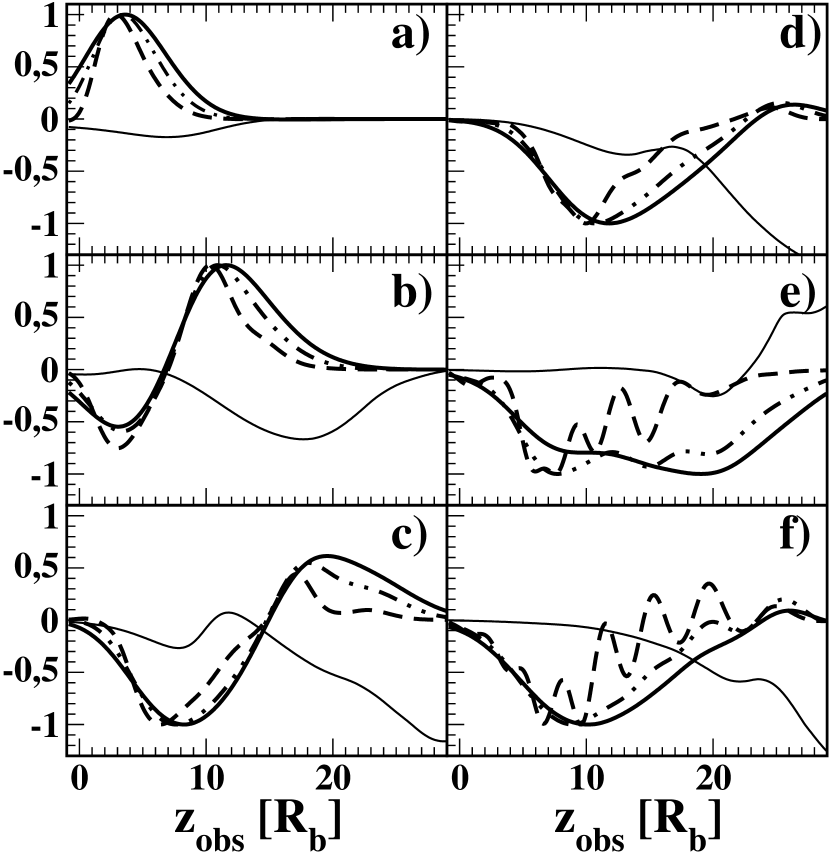
Figure 13.— In each panel lines correspond to the differences in intensity or spectral index between model PM-H with and without a hydrodynamic perturbation. Each panel corresponds to a different observer’s time (the times are the same as in Figs. 10 and 12). The thick-solid, dashed-dotted and dashed lines represent the normalized difference $(I^{p}(Z)-I(Z))/\max_{{}_{Z}}|I^{p}(Z)-I(Z)|$, at 15 GHz, 22 GHz and 43 GHz, respectively. $I(Z)$ and $I^{p}(Z)$ are the intensities averaged over cross-sections of the jet at each distance $Z$ from the injection nozzle for the quiescent and perturbed models, respectively. The maximum in the denominator extends for all $Z$ along the jet axis. The thin solid line shows the difference in the spectral index between the PM-H model with the hydrodynamic perturbation and the corresponding quiescent model. Precisely, the line shows the function $5\times(\alpha_{13}(Z)-\alpha_{13}^{p}(Z))/\max_{{}_{Z}}|\alpha_{13}(Z)|$, where $\alpha^{p}_{13}(Z)$ and $\alpha_{13}(Z)$ correspond to the cross-sectional average of the spectral index (Eq. 43) of the jet with the injected hydrodynamic perturbation and to the quiescent jet, respectively.

We have also checked that the profile outlined above does not depend on including synchrotron losses either. However, the smaller the magnetic field, the larger the increase in the spectral index behind the intensity maxima associated to the main component (i.e., associated with the rarefaction trailing the main hydrodynamic perturbation). The time evolution of the prototype spectral profile of a hydrodynamic perturbation injected at the nozzle is characterized by a substantial steepening of the spectrum behind the intensity maxima (Figs. 13c and  14c,d) compared to the quiescent jet model. This behavior of the spectral index has also been found in previous theoretical papers, and it is attributed to the fact that the NTP distribution evolves on timescales smaller than the light crossing time of the source (e.g., Chiaberge & Ghisellini, 1999).

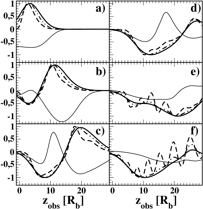
Figure 14.— Same as Fig.13 but for the model PM-L.

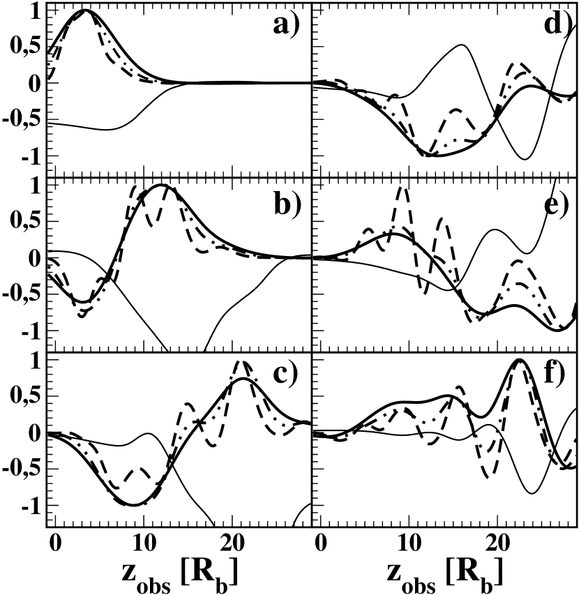
Figure 15.— Same as Fig.13 but for the model OP-L.

Comparing Figs. 13e and  14e, it is remarkable that trailing components pop up precisely to the left (i.e., behind) of the local relative spectral index minimum (at $Z\sim 18R_{b}$ in Fig. 14e and $Z\sim 20R_{b}$ in Fig. 13e) that follows the local relative maximum of the spectral index reached in the wake of the main perturbation. Furthermore, we notice that the intensity relative to the background jet of the trailing components identifiable at 43 GHz, depends on the strength of the initial magnetic field, in spite of the fact that in our models the magnetic field is dynamically negligible. At higher magnetic field strength the intensity of the trailing components is lowered and, some of them are hardly visible (e.g., the leading trailing at $\sim 25R_{b}$ is evident in Fig. 14f, while it is difficult to identify in Fig. 13f). Thereby, the observational imprint of trailing components is frequency dependent.

The evolution of the perturbation in model OP-L displays a slightly different profile at 43 GHz than in model PM-L. The main component splits into two sub-components at the highest observing frequency (Fig. 15b). At 15 GHz and 22 GHz, the profile of the perturbation is qualitatively the same as for the PM-L model. The spectral index displays a behavior very similar to that of the PM-L model. However, the evolution after the passage of the main component in model OP-L (Fig. 15d – 15f) is different from that of model PM-L. The number of bright spots popping up in the wake of the main perturbation is smaller and they are brighter (in relation to the quiescent jet) in the OP-L model than in the PM-L one. Identifying these features as trailing components (Sect. 7.2), we realize that they do not only appear at 43 GHz, but also at 22 GHz, and one may guess them even at 15 GHz.

7.2. Spacetime analysis

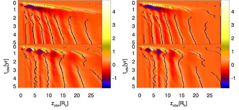
Figure 16.— Spacetime plot of the difference in the intensity at 43 GHz, averaged over the beam cross-section, between the perturbed and quiescent SPEV emission for PM-L and OP-L (upper left and lower left panels, respectively) and PM-H and OP-H (upper right and lower right panels, respectively) unconvolved models. The slope of the dashed line corresponds to an apparent velocity equal to the speed of light. The solid black dots correspond to the world-lines of a number of bright features observed in the convolved 43 GHz-radio images resulting from the difference between the hydrodynamic models with and without an injected perturbation. Among these features, there are trailing components (particularly in the PM models) and also standing recollimation shocks (characteristic of the OP models). The peaks in the color plot (yellow-white shades) do not always match the distribution of black dots due to the difference in the resolution of the convolved and unconvolved data. The color scale is linear and common for each column of panels. It displays the difference of averaged intensities in arbitrary units.

In order to relate the hydrodynamic evolution with the features observed in the synthetic radio maps, we have built up several space-time diagrams of the evolution of the component as seen by a distant observer. In Fig. 16 we plot the difference in intensity, averaged over the beam cross-section, between the perturbed and quiescent models. This difference accounts for the net effects that the passage of the hydrodynamic perturbation triggers on the quiescent jet. The trajectory of the main component is seen as a bright (yellow) region close to the top of each plot. Its superluminal motion is apparent when the slope of the trajectory is compared to that of the dashed line, which denotes the slope corresponding to the speed of light. Below the main component, the dark (blue) region is associated to the reduced intensity that the rarefaction trailing the hydrodynamic perturbation leaves.

As in G97, while in models PM-L and PM-H the main component and the reduced intensity region trailing it are continuous in the space-time diagrams (Fig. 16 upper panels), in OP-L and OP-H models they flash intermittently as they cross over standing cross shocks of the beam (larger intensity – Fig. 16 lower left panel) and then expand in the rarefactions that follow such standing shocks (smaller intensity). The interaction of the perturbation with the standing shocks of the quiescent OP model results in a displacement of the position of the shocks also noticed in G97. The temporarily dragging of standing components, is clearly visible in the lower left panel of Fig. 16. The second (from the left) of the well identified bright spots, oscillates with an amplitude of $\sim 1.4R_{b}$ in $\sim 10\,$months. The trend being to increase both the oscillation period and the amplitude with the distance to the jet nozzle.

Besides the main component, we observe several trailing components (Agudo et al., 2001), identified in Fig. 16 by “threads” with an intensity larger than in the quiescent model, which emerge from the wake of the main component. In Fig. 16 we also overplot (black dots) the world-lines of a number of bright features observed in the convolved 43 GHz-radio images resulting from the difference between the hydrodynamic models with and without an injected perturbation. These world-lines show only those local intensity maxima which could be unambiguously tracked in convolved radio maps. Except for the bright features closer to the jet nozzle, the world-lines match fairly well the unconvolved trails of high intensity. The latest three trailing components of Fig. 16 (upper left panel) do actually recede in the convolved 43 GHz maps as much as $0.5R_{b}$ for 1 to 4 moths, soon after they are identified (i.e., at an apparent speed $\sim 0.5c-0.9c$).

Figure 17.— World-lines of a number o bright features observed in the unconvolved radio images resulting from the difference between the hydrodynamic models with and without an injected perturbation (like in Fig. 16). Squares, triangles and crosses correspond to the radio frequencies 43 GHz, 22 GHz and 15 GHz, respectively. The size of the symbols is proportional to the wavelength of the data they display. Shown are PM-L and OP-L (upper left and lower left panels, respectively) and PM-H and OP-H (upper right and lower right panels, respectively) models. The slope of the dashed line corresponds to the an apparent velocity equal to the speed of light.

Like in the case of PM models, in the wake of the main component of model OP a number of bright spots seem to emerge with increasingly larger apparent velocities as they pop up far away from the jet nozzle. However, looking at the locations from where these components seem to emerge, we notice that they are in clear association with the locus of the standing shocks of the OP models. Such an association is even more evident when we look at the world-lines of the brighter features trailing the main component as they are localized in the 43 GHz radio maps. The physical origin of these trailing features differs from that of the trailing components seen in PM models. There trailing components are local increments of the pressure and of the rest-mass density of the flow produced by the linear growth of KH modes in the beam, generated by the passage of the main hydrodynamic perturbation. In the beam of OP models, intrinsically non-linear standing shocks are present. Nonetheless, the interaction of a non-linear hydrodynamic perturbation with non-linear cross shocks yields an observational trace which resembles much that of a trailing component. Thereby we keep calling such features trailing components, following Agudo et al. (2001).

If the jet is not pressure matched, all the KH modes excited in the beam are blended with standing knots. Indeed, we realize that close to the jet nozzle, the locus of the first two bright spots is almost standing and, at larger distances, the subsequent knots show a clear increment of its pattern speed. The fist two trailing components are, actually, the traces of standing shocks which are dragged along with the main perturbation and oscillate around their equilibrium positions. The remaining trailing components move much faster and they can probably be due to the pattern motion of KH modes in the OP beam.

Comparing the traces left by the passage of the main hydrodynamic perturbation in the PM and OP models (Fig. 16), it turns out that the signatures of such perturbation are much cleaner and numerous in PM than in OP models. The number of trailing components is smaller in OP than in PM models, and their world-lines are more oscillatory than in the latter case. For a lager magnetic field (models PM-H and OP-H; Fig. 16 right panels) NTPs cool faster and radiate more energy, and thus, one can basically see only features happening close to the jet nozzle.

The unconvolved data for both PM and OP models, and independently of the magnetic field strength, is compatible with not having any time lag between the high and low frequency radiation emitted by the main component, i.e., the radiation at all three frequencies is co-spatial (Fig. 17). However, the convolved data display a number of positive and negative time lags which result from the difference in the size of the convolution beam at every frequency. In case of the PM models, there is a trend of the 43 GHz maximum emission to lie behind the corresponding maxima at 22 GHz and 15 GHz (Fig. 18 upper panels). Thereby, the low energy radiation from the main component is seen first, and later an observer detects radiation at higher frequencies. Nevertheless, considering that the resolution of the convolved data is worse at smaller frequencies, the emission from the component is consistent with having no time-lags between low and high frequency emission. This trend is independent of the magnetic field strength, but it is more obvious for the model PM-H model (note the large separation between the different symbols beyond $Z_{\rm obs}\sim 15R_{b}$ in the Fig. 18 upper right panel). Therefore, any positive or negative time lag of radiation at different frequencies measured from convolved data has to be taken with care.

For OP-L models, positive and negative time lags between the high and low energy radiation are observed along the $z$-axis (Fig. 18 lower left panel). Such time lags are smaller than for the PM-H model and, indeed, the data are compatible with no-time lags at all. For OP-H, in most cases, the high-frequency emission dots lie in front of the lower frequency ones (Fig. 18 lower right panel). But still, considering the difference in linear resolution for the location of the maxima, the radiation at different frequencies is almost co-spatial.

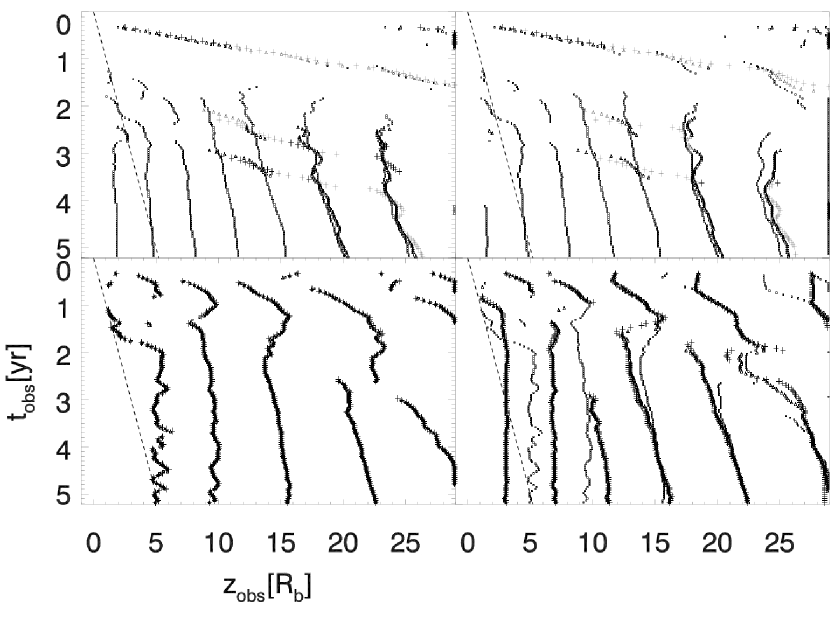
Figure 18.— Same as Fig. 17 but using convolved data at every frequency. The location of local maxima trailing the main perturbation in the beam of PM models is difficult at 15 GHz and 22 GHz because of the large convolution beam at these two frequencies. The low observing resolution at such frequencies drives spurious detections of local maxima in the radio maps (trailing components), which explain the anomalous data at 15 GHz and 22 GHz in the range $(t_{\rm obs},z_{obs})=(2\,{\rm yr}-3.7\,{\rm yr},10R_{b}-20R_{b})$ in the PM model (upper panels). The OP models do not display such obvious anomalies because the high intensity threads that trail the main perturbation are associated with preexisting recollimation shocks in the beam, whose emissivity, relative to the background jet, is much larger than that corresponding to the trailing components in the PM models.

Trailing components can only be tracked at 43 GHz close to the jet nozzle. Only after a certain distance, it is possible to see them at 22 GHz and even at 15 GHz (see the last two trailing world lines in each panel of Fig. 18). The world lines of trailing components at 22 GHz and, particularly, at 15 GHz, undergo substantial velocity changes. During some time intervals the convolved data shows receding trailing components at such frequencies. In the OP models, there are no clear trends, independent of the magnetic field strength, since it is very difficult to locate any local maxima at 15 GHz, and the 22 GHz data lie almost on top of the 43 GHz points. We note that there is a mismatch between the data points at different frequencies in the OP-H model at the first two recollimation shocks (vertical threads at $z_{\rm obs}\sim 4R_{b}$ and $7R_{b}$). It is produced because there is a rather small relative difference in the emissivity of the perturbed and the quiescent jet models at 43 GHz until $z_{\rm obs}\mathrel{\hbox to0.0pt{\lower 4.0pt\hbox{\hskip 1.0pt$\sim$}\hss}\raise 1.0pt\hbox{$<$}}10R_{b}$. In such conditions, the algorithm to detect local maxima in the space-time diagrams yields oscillatory results. A large mismatch between the world-lines of the peak intensity of trailing components at different frequencies also happens in other trailing features (e.g., the fourth and fifth threads in Fig. 18 lower right panel). This mismatch does not exist in the corresponding unconvolved data (Fig. 17) and, hence, we conclude it is an artifact of the finite size of the convolution beam at the observing frequencies.

8. Discussion and conclusions

We have presented a new method (SPEV) to compute the evolution of NTPs coupled to relativistic plasmas under the assumption that these NTPs do not diffuse across the underlying hydrodynamic fluid. NTPs change their energy because of the variable hydrodynamic conditions in the flow and because of their synchrotron losses in an assumed background magnetic field. The inclusion of synchrotron losses and a transport algorithm for NTPs are major steps forward with respect to previous approaches we have followed. The new method has been validated with another preexisting algorithm suited for the same purpose, but without including synchrotron losses and transport of NTPs (AM algorithm). The validation process shows that the SPEV method reproduces the same qualitative phenomenology as outlined in the previous works of our group (G95, G97). The power of the new method in its whole blossom shows up when synchrotron cooling dominates the NTP evolution.

Quiescent jet models:

When synchrotron losses are considered, the resulting phenomenology can be split into two regimes: losses-dominated and adiabatic regime (following the convention of Marscher & Gear, 1985). In the losses-dominated regime, the knots displayed in the radio maps, which are close to the jet nozzle, are brighter than in models which do not include synchrotron cooling at the considered frequencies. Indeed, quiescent jet models including radiative losses are more knotty than those models which do not include them. These features result from the conservation of the number density of NTPs. Since the same number of particles per unit of volume that initially extends from $\gamma_{\rm min}(t=0)$ to a certain upper limit $\gamma_{\rm max}(t=0)$ is confined into a narrower Lorentz factor interval, wherein more NTPs are efficiently emitting in the considered observational radio bands. In the adiabatic regime (reached relatively far away from the jet nozzle), the spectral changes, that the NTP population experiences as it is advected downstream the jet, of models with and without losses is qualitatively similar, since most of the high-energy NTPs (which evolve faster) have cooled down to energies where losses are negligible. The beam of the jet in the adiabatic regime is dimmer at radio-frequencies than in models where synchrotron losses are not included. Our method lacks of a suitable scheme to account for diffusive shock acceleration of NTPs. However, all shocks existing in the quiescent jet models are rather weak and, for practical purposes they can be considered as compressions in the flow, where an enhanced emission is obtained due to the local increase of density and of pressure.

One of the main results of this work is that for the same background hydrodynamic jet model, dynamically negligible magnetic fields of different strengths yield substantially different observed morphologies. This introduces a new source of degeneracy (in addition to relativistic effects, such as, time delay, aberration, etc.) when inferring physical parameters out of observations of radio jets. For example, the difference in the observational properties of models OP-L and OP-H (Sect. 5.2) shows, that increasing the magnetic field strength by a factor of 10 triggers a much faster cooling of the NTPs, resulting in a much shorter losses-dominated regime and shorter jets, despite magnetic field remaining dynamically unimportant. Furthermore, jet models with such a large magnetic field display a larger flux density contrast between shocked and unshocked jet regions. The reason being that after the losses-dominated regime, $\gamma_{\rm max}$ is reduced so much that most of the NTP population is inefficiently radiating at the considered radio wavelengths and, only when the non-thermal electrons are compressed at cross shocks of the beam, they partly reenter into the efficiently radiating regime at the considered frequencies.

Spectral inversion:

In this paper we suggest that an inverted spectrum may also result if the lower limit of the NTP distribution $\gamma_{\rm min}$ is larger than the value of $\gamma_{{}_{\rm M}}$ for which the synchrotron function $R(x)$ reaches its maximum (Eq. 44), in agreement with the theoretical predictions of Tsang & Kirk (2007). Evidences for flat, optically thin radio spectra in several active galactic nuclei have been shown by, e.g., Hughes, Aller & Aller (1989b); Melrose (1996), and Wang, et al. (1997). These authors consider different kinds of Fermi-like acceleration schemes to be responsible for the hardness of the electron energy spectra. Stawarz & Petrosian (2008) show that stochastic interactions of radiating ultrarelativistic electrons with turbulence characterized by a power-law spectrum naturally result in a very hard (actually inverted) electron energy distribution which yields a synchrotron emissivity at low frequencies with an spectral index $\simeq 1/3$. Alternatively, Birk, Crusius-Wätzel & Lesch (2001) argue that optically thin synchrotron emission due to hard electron spectra produced in magnetic reconnection regions may explain the origin of flat or even inverted spectrum radio sources. In contrast to our findings, these authors, explain the spectral inversion in some sources as a result of a flatter electron energy distribution. Observationally, it could be possible to discriminate between both possibilities by looking at the high-energy spectrum of the source. If there are external seed photons (e.g., from the AGN), which were Compton up-scattered by the non-thermal electrons of the jet, the spectral index at high energies could discriminate between the alternative explanations for the optically-thin inverted spectra at radio frequencies.

Since $\gamma_{\rm min}$ is fixed in our model through Eq. (38) and it is not derived from first principles, one may question whether the value we obtain for $\gamma_{\rm min}$ could be too large and, therefore, the spectral inversion we are explaining on the basis of taking $\gamma_{\rm min}\mathrel{\hbox to0.0pt{\lower 4.0pt\hbox{\hskip 1.0pt$\sim$}\hss}\raise 1.0pt\hbox{$>$}}\gamma_{{}_{\rm M}}$ is unlikely to happen in nature. This would be the case if the jet was composed by and electron-positron plasma, in which case $\gamma_{\rm min}\simeq 1$ (e.g.,Marscher, et al. 2007). For plasmas made out of electrons and protons, Wardle (1977) obtained that for synchrotron sources with a brightness temperature $\simeq 10^{12}\,$K and $q=2$, $\gamma_{\rm min}\mathrel{\hbox to0.0pt{\lower 4.0pt\hbox{\hskip 1.0pt$\sim$}\hss}\raise 1.0pt\hbox{$>$}}161$ in order to account for the low degree of depolarization in parsec-scale emission regions. More recently, Blundell, et al. (2006) inferred $\gamma_{\rm min}\sim 10^{4}$ at the hot-spots of 6C 0905+3955 (see also Tsang & Kirk 2007, and references therein). Thus, the exact value of $\gamma_{\rm min}$ is probably source dependent, and our minimum Lorentz factor threshold ($\gamma_{\rm min}\simeq 330$) can be well accounted by present day theory and observations if the jet is not a pure electron-positron plasma.

Radio components:

We have applied the SPEV method to calculate the spectral evolution of superluminal components in relativistic, parsec-scale jets. These components are set up as hydrodynamic perturbations at the jet nozzle. For a small value of the magnetic field (the same as in G97), synchrotron losses are negligible and we recover the phenomenology shown by G97 and Agudo et al. (2001).

The main component is characterized by a hardening of the spectrum. Pressure matched models yield a generic spectral profile of the component, which is rather independent of synchrotron losses. The hydrodynamic perturbation looks in the radio maps like a burst at every radio-frequency and, just behind it, there is a decrease of the flux density. The shape of the burst is asymmetric in the axial jet direction, being brighter upstream than downstream. The shape of the burst is also frequency dependent because the convolution beam grows linearly with the observing wavelength (at lower frequencies the component is more symmetric in the axial jet direction). This triggers a decrease of the spectral index in the forward region of the main component, until it reaches a minimum (which precedes the intensity maxima at the highest observing frequency).

When radiative losses are important, a number of differences can be observed:

1. Main component splitting in OP-H model: The main component splits in the radio-maps much more clearly than in OP-L model (Sect. 7.1), and the splitting takes place farther away from the nozzle in the latter than in the former case. The rear part of the component is brighter than the forward one if losses are included. The spectral index profile is unaffected by the apparent splitting of the component. We conclude that the apparent splitting of the main component is an artifact of the sampling of the results in the observer frame. It is necessary to perform a finer time sampling of the radio jet than the $\sim 3.5\,$months we have considered in the radio maps, in which case, the main component exhibits an intermittent variation of its flux density (see on line material). If observations do not have the sufficient time resolution, there is another hint that can help to disentangle whether the splitting is apparent or real. In a true splitting of the component, each part may show a different spectral aging due to their different hydrodynamic evolutions.

2. Radio features: Main and trailing components display a less elongated aspect in radio maps. The reason is that without losses, the beam itself is brighter at longer distances. Thus, in the unconvolved data, the parts located downstream the jet weight more in the convolution beam than in the case where synchrotron losses are included. For the same reason, models which include synchrotron losses display a more knotty morphology. In the losses-dominated regime, SPEV models exhibit a brighter main superluminal component than SPEV-NL models. This behavior reverses in the adiabatic regime. Also, the ratio between the peak specific intensity of a trailing component to the specific intensity of the region of the beam immediately behind it, is larger than if losses are not included. The conservation of the NTPs number density explains this phenomenology (Sect. 5.2.1).

3. Spectral properties: Behind the main component, the spectral index returns almost monotonically to its unperturbed value. In contrast, when losses are negligible, there is a softening of the spectrum, just behind the main component (where the spectral index reaches a maximum).

Time lags:

In this paper we explicitly show, that the convolved data has to be interpreted carefully. During most of the time the main component is observable, the radiation emitted by the component at low energy (15 GHz) arrives to the observer before that at high energy (43 GHz). Indeed, for models PM-H and OP-H, a substantial mismatch between the world-lines of the peak intensity of trailing components at different frequencies is possible. This mismatch is an artifact due to the finite size of the convolution beam at the observing wavelengths.In contrast, the unconvolved data is consistent with a simultaneous emission of radiation at the three frequencies under consideration. This behavior matches our expectations, since the interval of observing wavelengths is too narrow to display a substantial frequency dependent separation of the regions of maximum emission.

On the nature of trailing components:

The journey of the main component downstream the jet generates a number of frequency dependent bright spots which pop up in its wake. They differentiate themselves from the main component because (1) they do not emerge from the jet core, (2) they posses substantially smaller (sometimes subluminal or even, receding) speeds (Agudo et al., 2001) and, as we demonstrate here, (3) they do not exhibit an obvious change in the spectral index with respect to the quiescent jet model, but (4) their observational imprint is frequency dependent (they are clearly visible at the highest radio-observing frequencies, but at 22 GHz and, particularly, at 15 GHz they are wiped out by the large convolution beams at this wavelengths). In pressure matched jet models, trailing components result from the linear growth of KH modes in the beam, after the passage of the main hydrodynamic perturbation (Agudo et al., 2001). Here, we also consider overpressured jet models, where the situation is qualitatively different from pressure matched ones, since the beam of such models develops standing shocks (non-linear structures). Nonetheless, the interaction of a non-linear hydrodynamic perturbation with non-linear cross shocks yields an observational trace which resembles that of a trailing component. Therefore, sticking to the definition of Agudo et al. (2001), we also call trailing components to the bright spots following the main component in overpressured models, although the dynamical origin of such components differs. In this sense, every bright spot that results from the interaction between a strong hydrodynamic perturbation with a relativistic beam, which moves slower than the main component and is not ejected from the jet core shall be considered as a trailing component. We shall add an obvious cautionary note: striving for the knowledge of the jet parameters, on the basis of a fit of the intensity variations behind a main perturbation to a number or KH modes, requires that the jet is pressure matched (if the jet is not pressure matched, all the KH modes excited in the beam are blended with standing knots and the predicted jet parameters might be inaccurate). Furthermore, it is necessary that the linear resolution of the convolved (observational) data was rather good. We have tested that the unconvolved results are roughly recovered if the FWHM of the beam at 43 GHz is smaller than $0.25R_{b}$. Insufficient linear resolution biases the observed features in hardly predictable ways, rendering inadequate the identification of features in the radio maps with hydrodynamic structures.

In the future we plan to apply the SPEV method to perform additional parametric studies of relativistic parsec scale jets. Among the parameters which can be interesting to look at, we give preference to the electron spectral index. Also, the SPEV algorithm can be coupled to relativistic magnetohydrodynamic codes. This will drop any assumption about the topology and strength of the magnetic field in the jet, and it will enable us to perform also parametric studies of polarization of the jet emission and of superluminal components.

Appendix A A. Imaging algorithm

Equations given in Secs. 3 and 4 are, in principle, sufficient to compute the synchrotron emissivity at any position in space and at any instant of time in the observer’s frame, either using SPEV or AM methods, accounting for the appropriate transformations from the frame comoving with the fluid (where the emissivity [Eq. 39], absorption coefficient [Eq. 4], number density of NTPs [Eq. 5], etc. are computed).The purpose of this Appendix is to explain the algorithm used to produce synthetic radio maps from discrete spatial and temporal elements.

A.1. Geometry and arrival time

While in our simulations the hydrodynamic state of the fluid is axisymmetric regardless of the jet viewing angle, the observed emission is, in general, not axisymmetric. We introduce the azimuthal angle $\phi$ (measured in the $xy$-plane from the $x$-axis) and define the laboratory frame (attached to the center of the AGN) 3D Cartesian coordinate system $(x,y,z):=(R\cos\phi,R\sin\phi,Z)$, where the $z$-axis coincides with the jet axis. We denote the jet viewing angle by $\theta$, and choose the following observer coordinate system (rotated with respect to the 3D Cartesian system by an angle $\theta$ around the $y$-axis)

$$(x_{\rm obs},y_{\rm obs},z_{\rm obs}):=(x\cos\theta+z\sin\theta,y,-x\sin\theta+z\cos\theta)\,$$ (A1)

in which the observer is located along the $z_{\rm obs}$ axis, far from the jet. For a given elapsed simulation time $T$ in the jet frame the time of observation $t_{\rm obs}$ is defined as

$$t_{\rm obs}:=T-z_{\rm obs}/c$$ (A2)

The task of the imaging algorithm is to produce image in the $(x_{\rm obs},y_{\rm obs})$ plane for a fixed arrival time $t_{\rm obs}$ (note that the image will be symmetric with respect to the $x_{\rm obs}$-axis if the magnetic field is completely random). From Eqs. A1 - A2 it is clear that we need to have information about states of the jet at multiple instants of laboratory frame time in order to correctly compute the contribution at a single $t_{\rm obs}$. In a numerical hydrodynamic simulation we only have a finite number of discrete iterations, but each iteration has an associated time step $\Delta T$. In order to correctly take this into account, in the following we assume that the time instant $t_{\rm obs}$ has a finite duration $\Delta T$ as well, and all radiation arriving between $t_{\rm obs}-\Delta T/2$ and $t_{\rm obs}+\Delta T/2$ is arriving precisely at $t_{\rm obs}$.

A.2. Particle images

Owing to the axisymmetric nature of the problem, we only follow the Lagrangian particle motion and evolution in two dimensions (see Sec. 3). However, for the purposes of imaging, a three-dimensional particle distribution needs to be created. We assume that each particle which is injected at the jet nozzle has a radius $\Delta r:=R_{\rm b}/(2N_{\rm p})$, where $R_{\rm b}$ is the beam radius and $N_{\rm p}$ number of particles per beam radius. That means that a particle in two dimensions correspond to a revolution annulus in the $(x,y,z)$ coordinate system. In principle, by knowing the particle position $(R_{\rm p},Z_{\rm p})$ in the 2D grid we could compute from Eqs. A1 - A2 all combinations of $(x,y,z)$ and, hence, all combinations $x_{\rm obs}$, $y_{\rm obs}$ and $t_{\rm obs}$ to which the particle annulus corresponds for a fixed $T$. In practice, we approximate every annulus by a series of cubes which are distributed along a circle with radius $R_{\rm p}$, whose center is in $(0,0,Z_{\rm p})$. The number of cubes, evenly distributed in the azimuthal direction, necessary for an optimal volume coverage of the annulus depends on the relation between $R_{\rm p}$ and the particle radius $\Delta r$ (see next subsection). By virtue of the symmetry of the jet, as seen by the observer, with respect to the $x_{\rm obs}$-axis, we only need to compute the contribution from one half-annulus, i.e. for those cubes where $y=y_{\rm obs}\geq 0$.

We assume that both the emissivity and the absorption coefficient are homogeneous within each cube. Thus, knowing the particle velocity and the azimuthal angle of a given cube, we can transform its emissivity and its absorption into the observer frame.

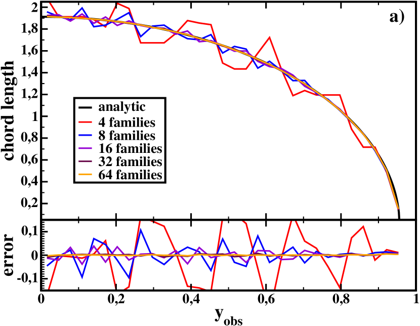
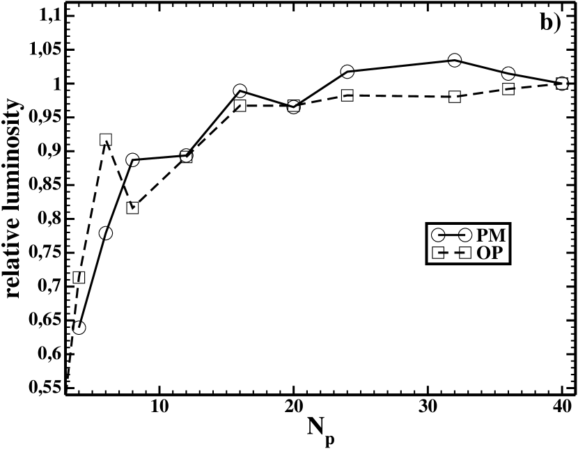
Figure 19.— Left: Results of the volume filling convergence test for different numbers of particles per unit of beam radius $N_{\rm p}$. In the upper panel we show the computed length of the chord through the jet as a function of the height $y_{\rm obs}$. We fix the value of the jet radius to be $R_{\rm b}=0.95625$. The thick black line corresponds to the analytic expectation of the chord length, i.e., $2\sqrt{R_{rmb}^{2}-y_{\rm obs}^{2}}$. In the lower panel the relative error with respect to the analytic expectation is displayed. Right: Results of the flux convergence test. The figure displays the total flux of images at $15\,$GHz for the quiescent PM (circles) and OP (squares) models as a function of the number of particles per beam radius $N_{\rm p}$ injected at the jet nozzle. Images have been produced with 4, 8, 16, 20, 24, 32 and 40 particles per beam radius. The luminosity of both families of models are normalized to the total flux produced by the corresponding (PM or OP) model with $N_{\rm p}=40$.

A.2.1 Approximation of annuli by cubes

Given a particle with radius $\Delta r$ and cylindrical coordinates $(R_{\rm p},Z_{\rm p})$, we approximate the corresponding half-revolution annulus by cubes evenly tessellating a circumference centered at $(0,0,Z_{\rm p})$. The angular separation between the cubes is defined as $\Delta\phi=\min{(\pi,2\Delta r/R_{\rm p})}$. Thus, there are $N_{\phi}=\pi/\Delta\phi=\max{(1,R_{\rm p}\pi/(2\Delta r))}$ cubes in a half-annulus of volume $V_{\rm cubes}=N_{\phi}(2\Delta r)^{3}=4\pi R_{\rm p}(\Delta r)^{2}$ whereas the true volume of the half-annulus is

$$V_{{}_{\rm HA}}=\left\{\begin{array}[]{rl}[(R_{\rm p}+\Delta r)^{2}-(R_{\rm p}-\Delta r)^{2}]\pi(2\Delta r)/2=4\pi R_{\rm p}(\Delta r)^{2}&\rm{if\ }R_{\rm p}>\Delta r\\[11.38109pt] (R_{\rm p}+\Delta r)^{2}\pi(2\Delta r)/2=(R_{\rm p}+\Delta r)^{2}\pi\Delta r&\rm{if\ }R_{\rm p}\leq\Delta r\end{array}\right.$$ (A3)

In the limit of $R_{\rm p}>\Delta r$, the total volume of the cubes is approximating that of the half-annulus. For $R_{\rm p}<\Delta r$, $N_{\phi}$ is reset to $1$ and the volume for which $y>0$ is always $4(\Delta r)^{3}$, which is close to the average over all possible values $R_{\rm p}\leq\Delta r$ of the true volume $7\pi(\Delta r)^{3}/6$.

A.3. Radiative transfer

To compute an image we subdivide the $(x_{\rm obs},y_{\rm obs})$ plane into rectangular pixels, and compute the contributions to each pixel by checking which particle cube intersects which pixel at the right observation time. The ratio of the area of intersection to the pixel area, gives a “weight” of the contribution of a particular cube to the intensity of the pixel. For a given $T$, the value of $z_{\rm obs}$ for each particle gives the distance from the observer, so that we create a “line-of-sight” (LoS) for each pixel and sort along this line all contributing particles according to $z_{\rm obs}$ (note that these contributions generally come from different instants of the laboratory frame time $T$). Since in every pixel we sum up the contributions spanning the observer time range $[t_{\rm obs}-\Delta T/2,t_{\rm obs}+\Delta T/2]$, the intersections of every LoS with particle cubes are segments, not points (which would be the case if in every pixel we would only consider the instantaneous contributions at $t_{\rm obs}$). After all the contributions (i.e., intersection segments) to a pixel have been accounted for, we solve the standard radiative transfer equation to evaluate the final pixel intensity. The above procedure can be performed simultaneously for a number of different values of $t_{\rm obs}$, so that a “movie” in the observer frame can be created. In order to transform the intensity detected in a pixel into a flux we need to multiply by the pixel area.

A.4. Tests of the method

In order to validate our imaging algorithm we have developed two tests which are based upon the idea that, increasing the number of Lagrangian particles, both the volume filling factor and the total detected flux should converge. We first show the convergence of the volume filling method. Then we show that the images and the total flux of the quiescent PM-L and OP-L models converge with increasing number of particle families.

A.4.1 Volume filling

We have created a toy model consisting of a cylindrical jet with uniform velocity parallel to the jet axis, and with a length equal to the particle size $\Delta r$. The half-volume of such jet is $V_{\rm j,1/2}=\pi R_{\rm b}^{2}\Delta r$. We inject $N_{\rm p}$ particles in the jet evenly distributed across the jet radius (i.e., $\Delta r=R_{\rm b}/(2N_{\rm p})$, or $R_{\rm b}=(2i+1)\Delta r$, $i=0,\dots,N_{\rm p}-1$). If particles do not overlap, the volume filling factor is

$$\frac{\sum_{i=0}^{N_{\rm p}-1}V_{{\rm cubes},i}}{V_{\rm j,1/2}}=\frac{\sum_{i=0}^{N_{\rm p}-1}4\pi(2i+1)(\Delta r)^{3}}{\pi R_{\rm b}^{2}\Delta r}=1-\frac{1}{N_{\rm p}}\,.$$ (A4)

Since we have a finite number of particles, the jet volume is only partially patched by the volume occupied by such Lagrangian particles, i.e., the volume filling factor is smaller than one. Increasing the number of particles brings it closer to one. To test the volume filling method, we produce an “image” of the jet at an observer time $t_{\rm obs}=0$ with a $90^{\circ}$ viewing angle, accumulating in each pixel the contributions corresponding to a laboratory frame time interval $\Delta T=2R_{\rm b}/c$. However, instead of summing up the emissivity, we add up the length of the intersection of each particle’s volume with each pixel in the $(x_{\rm obs},y_{\rm obs})$ plane (as described above). The idea behind the substitution of the emissivity by the intersection length is that, at $90^{\circ}$ the intersection length and the intersection volume of the particles are proportional and, thus, measuring lengths or volumes is equivalent.

Since we accumulate in every pixel all contributions in the range $[-\Delta T/2,\Delta T/2]$, the intersection length with each particle equals the size of the particle perpendicular to the LoS ($2\Delta r$). Hence, the value accumulated in a pixel ${\cal P}:=(x_{\rm obs},y_{\rm obs})$, namely $L_{\rm px}$, is

$$L_{\rm px}=\sum_{i}\frac{A_{i}}{A_{\rm px}}2\Delta r\,,$$ (A5)

where $A_{i}$ and $A_{\rm px}$ are the area of intersection of a particle with a pixel and the pixel area, respectively. The sum in Eq. (A5) extends over all particles that are intersected by the line of sight that departs from ${\cal P}$. In the limit $\Delta r\rightarrow 0$ (equivalently, $N_{\rm p}\rightarrow\infty$) $A_{i}\rightarrow 4(\Delta r)^{2}$. On the other hand, the number of particles intersected by the LoS departing from ${\cal P}$ and having a cross sectional area $A_{\rm px}$ is $N_{\rm px}=A_{\rm px}/(2\Delta r)^{2}$. Therefore, we have

$$\lim_{\Delta r\rightarrow 0}L_{\rm px}=\lim_{\Delta r\rightarrow 0}8(\Delta r)^{3}\frac{N_{\rm px}}{A_{\rm px}}=2\sqrt{(R_{\rm b}^{2}-y_{\rm obs}^{2})}\,.$$ (A6)

Equation A6 simply expresses that, in the limit $N_{\rm p}\rightarrow\infty$, the length measured in the pixel ${\cal P}$ should tend to the length of the chord determined by the intersection of the jet body with the line of sight from ${\cal P}$. Figure 19a shows that for $N_{p}\geq 16$ the results converge very rapidly to the analytic expectation (thick black line).

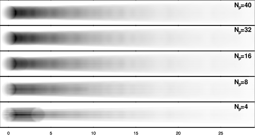
Figure 20.— Images of PM-L models used in the convergence test. From top to bottom $N_{p}=40$, $32$, $16$, $8$ and $4$.

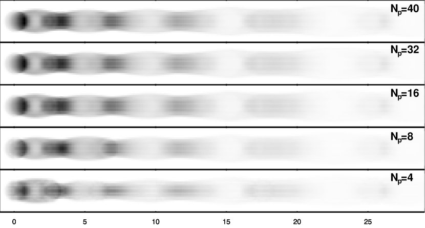
Figure 21.— Same as Fig. 20, but for the OP-L model.

A.4.2 Total flux

To test the convergence of the imaging algorithm we have produced images of quiescent PM-L and OP-L models with varying $N_{p}$. The total number of particles in the grid grows as $N_{\rm p}^{2}$, it is thus important to minimize the number of particle families for numerical purposes. On Fig. 19b we show the total image flux at $15$ GHz for PM-L and OP-L models as a function of $N_{\rm p}$. The values are normalized to the flux of the model with the largest number of injected particles per beam radius ($N_{\rm p}=40$), which we consider the reference value. This test is important because the total flux represents a global value of every model, since it is computed by summing up the individual fluxes arriving to each pixel in the detector, and multiplying by the corresponding pixel area. Remarkably, for $N_{\rm p}\geq 16$ the flux does not deviate more than $5\%$ form the reference value. Thus, any model with $N_{\rm p}\geq 16$ has sufficiently converged to an appropriate total flux. This has motivated our choice to work with $N_{\rm p}=32$ in the current paper, since it yields an optimal trade-off between numerical accuracy and computational cost. Figures 20 and 21 show images corresponding to the convergence tests for models PM-L and OP-L, respectively.

References

- Agudo et al. (2001) Agudo, I., Gómez, J. L., Martí, Ibáñez, J. M., Alberdi, A., Aloy, M. A., & Hardee, P. E. 2001, ApJ, 549, L183
- Aloy, Pons & Ibáñez (1999) Aloy, M. A., Pons, J. A., Ibáñez, J. M. 1999, Comp. Phys. Comm., 120, 115
- Aloy, et al. (1999) Aloy, M. A., Ibáñez, J. M., Martí, J. M., & Müller, E. 1999, ApJS, 122, 151
- Aloy, et al. (2003) Aloy, M. A., Martí, J. M., Gómez, J. L., Agudo, I., Müller, E., & Ibáñez, J. M. 2003, ApJ, 585, L109
- Achterberg, et al. (2001) Achterberg, A., Gallant, Y. A., Kirk, J. G., & Guthmann, A. W. 2001, MNRAS, 328, 393
- Blundell, et al. (2006) Blundell, K., Fabian, A., Crawford, C., Erlund, M., & Celotti, A. 2006, ApJ, 644, 13
- Blandford & Königl (1979) Blandford, R. D. & Königl, A. F. 1979, ApJ, 232, 34
- Blandford & McKee (1976) Blandford, R. D. & McKee, C. F. 1976, PhFl, 19, 1130
- Casse & Marcowith (2003) Casse, F. & Markowith, A. 2003, A&A, 404, 405
- Chiaberge & Ghisellini (1999) Chiaberge, M. & Ghisellini, G. 1999, MNRAS, 306, 551
- Daly & Marscher (1988) Daly, R. A. & Marscher, A. P. 1988, ApJ, 334, 34
- Duncan, Hughes & Opperman (1996) Duncan, G. C., Hughes, P. A., & Opperman, J. 1996, in ASP Conf. 100, Energy Trnasport in Radio Galaxies and Quasars, eds. P. E. Hardee, A. H. Bridle & J. A. Zensus, p. 143
- Gómez (2002) Gómez, J. L. 2002, LNP, 589, 169
- Gómez (2005) Gómez, J. L. 2005, ASP Conf. Proc., 340, 13
- Gómez, Alberdi & Marcaide (1993) Gómez, J. L., Alberdi, A., & Marcaide, J. M. 1993, A&A, 274, 55
- Gómez, Alberdi & Marcaide (1994) Gómez, J. L., Alberdi, A., & Marcaide, J. M. 1994, A&A, 284, 51
- Gómez, et al. (1994) Gómez, J. L., Alberdi, A., Marcaide, J. M., Marscher, A. P., & Travis, J. P. 1994, A&A, 292, 33
- Gómez, et al. (1995) Gómez, J. L., Martí, J. M., Marscher, A. P., Ibáñez, J. M. & Marcaide, J. M. 1995, ApJ, 449, L19 (G95)
- Gómez, et al. (1997) Gómez, J. L., Martí, J. M., Marscher, A. P., Ibáñez, J. M. & Alberdi, A. 1997, ApJ, 482, L33 (G97)
- Gómez, et al. (2000) Gómez, J. L., Marscher, A. P., Alberdi, A., Jorstad, S. G., García-Miró, C. 2000, Science, 289, 2317
- Gómez, et al. (2001) Gómez, J. L., Marscher, A. P., Alberdi, A., Jorstad, S. G., Agudo, I. 2001, ApJ, 561, L161
- Gómez, et al. (2008) Gómez, J. L., Agudo, I., Marscher, A. P., Jorstad, S. G., Roca-Sogorb, M. 2008, ApJ, 681, L69
- Heinz & Begelman (1997) Heinz, S., Begelman, M. C. 1997, ApJ, 490, 653
- Hughes, Aller & Aller (1985) Hughes, P. A., Aller, H. D., & Aller, M. F. 1985, ApJ, 298, 301
- Hughes, Aller & Aller (1989a) Hughes, P. A., Aller, H. D., & Aller, M. F. 1989a, ApJ, 341, 54
- Hughes, Aller & Aller (1989b) Hughes, P. A., Aller, H. D., & Aller, M. F. 1989b, ApJ, 341, 68
- Hughes, Aller & Aller (1991) Hughes, P. A., Aller, H. D., & Aller, M. F. 1991, ApJ, 374, 57
- Jones (1988) Jones, T. W. 1988, ApJ, 332, 678
- Jones & Kang (2005) Jones, T. W., & Kang, H. 2005, Astroparticle Phys., 24, 75
- Jones, Ryu & Engel (1999) Jones, T. W., Ryu, D., & Engel, A. 1999, ApJ, 512, 105
- Kirk (1994) Kirk, J. G. 1994, Saa-Fee Advanced Course: Plasma Astrophysics, eds. Benz, A. O. & Courvoisier, T. J.-L., Springer-Verlag, 225
- Königl (1981) Königl, A. 1981, ApJ, 243, 700
- Komissarov & Falle (1996) Komissarov, S. S., & Falle, S. A. E. G. 1996, in ASP Conf. 100, Energy Trnasport in Radio Galaxies and Quasars, eds. P. E. Hardee, A. H. Bridle & J. A. Zensus, p. 173
- Kraft, Forman, Jones & Murray (2001) Kraft, R. P., Forman, W. R., Jones, C., Murray, S. S. 2001, Bulletin of the American Astronomical Society, 33, 811
- Lobanov & Zensus (2001) Lobanov, A. P., & Zensus, J. A. 2001, Science, 294, 128
- Marshall, et al. (2002) Marshall, H. L., Miller, B. P., Davis, D. S., Perlman, E. S., Wise, M., Canizares, C. R., Harris, D.E. 2002, ApJ, 564, 683
- Marscher (1980) Marscher, A. P. 1980, ApJ, 235, 386
- Marscher & Gear (1985) Marscher, A. P., & Gear, W. K. 1985, ApJ, 298, 114
- Marscher, Gear & Travis (1992) Marscher, A. P., Gear, W. K., & Travis, J. P. 1992, in Variability of Blazars, eds. E. Valtaoja, & M. Valtonen (Cambridge: Cambridge Univ. Press), 85
- Marscher, et al. (2002) Marscher, A.P., Jorstad, S. G., Gómez, J. L., Aller, M. F., Teräsranta, H., Lister, M. L., Stirling, A. M. 2002, Nature, 417, 625
- Marscher, et al. (2007) Marscher, A.P., Jorstad, S. G., Gómez, J. L., McHardy, I. M., Krichbaum, T. P., Agudo, I. 2007, ApJ, 665, 232
- Marscher, et al. (2008) Marscher, A. P., Jorstad, S. G., D’Arcangelo, F. D., Smith, P. S., Williams, G. G., Larionov, V. M., Oh, H., Olmstead, A. R., Aller, M. F., Aller, H. D., McHardy, I. M., Lähteenmäki, A., Tornikoski, M., Valtaoja, E., Hagen-Thorn, V. A., Kopatskaya, E. N., Gear, W. K., Tosti, G., Kurtanidze, O., Nikolashvili, M., Sigua, L., Miller, H. R., Ryle, W. T. 2008, Nature, 452, 966
- Melrose (1996) Melrose, D. B. 1996, in IAU Symp. 175, Extragalactic Radio Sources, ed. R.Ekers, C. Fanti, & L. Padrielli (Dordrecht: Reidel), 423
- Micono, et al. (1999) Micono, M., Zurlo, N., Massaglia, S., Ferrari, A., Melrose, D. B. 1999, A&A, 349, 323
- Mimica (2004) Mimica, P., 2004, Ph.D. Thesis.
- Mimica, et al. (2004) Mimica, P., Aloy, M. A., Müller, E., & Brinkmann, W. 2004, A&A, 418, 947
- Mimica, et al. (2005) Mimica, P., Aloy, M. A., Müller, E., & Brinkmann, W. 2005, A&A, 441, 103
- Mimica, Aloy & Müller (2007) Mimica, P., Aloy, M. A., & Müller, E. 2007, A&A, 466, 93
- Miniati (2001) Miniati, F. 2001, Comp. Phys. Comm., 141, 17
- Miralles, van Riper & Lattimer (1993) Miralles, J. A., van Riper, K. A., Lattimer, J. M. 1993, ApJ, 407, 687
- Pacholczyk (1970) Pacholczyk, A. G. 1970, Radio Astrophysics.
- Perlman, et al. (2006) Perlman, E. S., Padgett, C. A., Georganopoulos, M., Sparks, W. B., Biretta, J. A., O’Dea, C. P., Baum, S. A., Birkinshaw, M., Worrall, D. M., Dulwich, F., Jester, S., Martel, A., Capetti, A., Leahy, J.P. 2006, ApJ, 651, 735
- Rees (1978) Rees, M. J. 1978, MNRAS, 184, 61P
- Rybicki & Lightman (1979) Rybicki, G. B., & Lightman, A. P. 1979, Radiative Processes in Astrophysics, Wiley Interscience
- Stawarz & Petrosian (2008) Stawarz, L., Petrosian, V. 2008, ApJ, 681, 1725
- Tregillis, Jones & Ryu (2001) Tregillis, I. L., Jones, T. W., & Ryu, D. 2001, ApJ, 557, 475
- Tsang & Kirk (2007) Tsang, O., & Kirk, J. G. 2007, A&A, 463, 145
- Wang, et al. (1997) Wang, J., Cen, X., Xu, J., & Qian, T. 1997, ApJ, 491, 501
- Wardle (1977) Wardle, J.F.C. 1977, Nature, 269, 563
- Webb (1985) Web, G. M. 1985, ApJ, 296, 319