Atmospheric Escape from Hot Jupiters

Abstract

Photoionization heating from UV radiation incident on the atmospheres of hot Jupiters may drive planetary mass loss. Observations of stellar Lyman-$\alpha$ absorption have suggested that the hot Jupiter HD 209458b is losing atomic hydrogen. We construct a model of escape that includes realistic heating and cooling, ionization balance, tidal gravity, and pressure confinement by the host star wind. We show that mass loss takes the form of a hydrodynamic (“Parker”) wind, emitted from the planet’s dayside during lulls in the stellar wind. When dayside winds are suppressed by the confining action of the stellar wind, nightside winds might pick up if there is sufficient horizontal transport of heat. A hot Jupiter loses mass at maximum rates of $\sim$$2\times 10^{12}{\rm\,g}{\rm\,s}^{-1}$ during its host star’s pre-main-sequence phase and $\sim$$2\times 10^{10}{\rm\,g}{\rm\,s}^{-1}$ during the star’s main sequence lifetime, for total maximum losses of $\sim$0.06% and $\sim$0.6% of the planet’s mass, respectively. For UV fluxes $F_{\rm UV}\lesssim 10^{4}{\rm\,erg}{\rm\,cm}^{-2}{\rm\,s}^{-1}$, the mass loss rate is approximately energy-limited and scales as $\dot{M}\propto F_{\rm UV}^{0.9}$. For larger UV fluxes, such as those typical of T Tauri stars, radiative losses and plasma recombination force $\dot{M}$ to increase more slowly as $F_{\rm UV}^{0.6}$. Dayside winds are quenched during the T Tauri phase because of confinement by overwhelming stellar wind pressure. During this early stage, nightside winds can still blow if the planet resides outside the stellar Alfvén radius; otherwise, even nightside winds are stifled by stellar magnetic pressure, and mass loss is restricted to polar regions. We conclude that while UV radiation can indeed drive winds from hot Jupiters, such winds cannot significantly alter planetary masses during any evolutionary stage. They can, however, produce observable signatures. Candidates for explaining why the Lyman-$\alpha$ photons of HD 209458 are absorbed at Doppler-shifted velocities of $\pm$100 km/s include charge-exchange in the shock between the planetary and stellar winds.

1. INTRODUCTION

About 1/5 of the approximately 200 extrasolar planets discovered to date have masses comparable to Jupiter’s, but orbit their host stars at distances less than 0.1 AU (e.g., Butler et al., 2006). Since stellar heating inhibits the formation of gas giants around Sun-like stars at such distances (e.g., Rafikov, 2006), these “hot Jupiters” likely migrated inward by disk torques from where they were born (e.g., Papaloizou et al., 2007, and references therein).

Once parked (possibly because the disk was truncated by the stellar magnetosphere; Lin et al. 1996), hot Jupiters are bathed in ultraviolet (UV) radiation from their host stars. Atmospheric gas is heated by photoionization of hydrogen, and escapes. Several groups have argued that the outflows can evaporate gas giants nearly entirely, laying bare their rocky cores (Lammer et al., 2003; Baraffe et al., 2004, 2005). In fact, hot Jupiters are observed to have systematically lower masses than extrasolar planets at larger distances from their stars (Zucker & Mazeh, 2002). However, Hubbard et al. (2007a, b) are unable to reproduce the mass distribution of hot Jupiters by experimentation with mass loss histories.

Observations of HD 209458b, the first hot Jupiter observed to transit its host star (Henry et al., 2000; Charbonneau et al., 2000), suggest that the planet may indeed be losing atomic hydrogen. Vidal-Madjar et al. (2003) used the Hubble Space Telescope Imaging Spectrograph (STIS) in a high spectral resolution mode to measure Lyman-$\alpha$ emission from HD 209458b’s host star in and out of transit. They observed, with $3\sigma$ confidence, the Ly$\alpha$ flux—at wavelengths shifted from line center by Doppler equivalent velocities of $\pm 100{\rm\,km}{\rm\,s}^{-1}$—to decrease during transit by $\sim$15% (as integrated over Doppler equivalent velocities extending approximately from -50 to -140 km/s and from +30 to +100 km/s). The authors attributed this decrease to absorption by intervening atomic hydrogen surrounding the planet: a halo of gas sufficiently distended and traveling at fast enough velocities to no longer be bound to the planet. The absorption signal was reported to be stronger at blueshifted wavelengths than at redshifted wavelengths; blueshifted velocities (towards the observer, away from the star) were argued to arise from stellar radiation pressure acting on gas via the Ly$\alpha$ line.

Ben-Jaffel (2007) reanalyzed the STIS data and agreed that stellar Ly$\alpha$ photons were absorbed by planetary gas during transit, but found the signal to be weaker: the flux decreased by only $8.9\pm 2.1$%, at similar Doppler equivalent velocities of $\pm$100 km/s. Moreover, no preference for blueshifted absorption was found. Ben-Jaffel (2007) cautioned that intrinsic stellar variability could easily produce a spurious preference for either negative or positive velocities. Despite this and other complications, Ben-Jaffel (2007) decided nonetheless that the absorption signal could be of planetary origin. From the effective occulting area corresponding to an 8.9% drop in flux, it was concluded that the obscuring hydrogen, while occupying a “corona” significantly more inflated than the visible photosphere, remained bound within the planet’s Roche lobe. This last argument, as pointed out by Vidal-Madjar et al. (2008), is not secure. If the wavelength shifts associated with the putative absorption reflect Doppler shifts from bulk flows, then the relevant velocities, regardless of whether they are positive or negative, are larger than the planet’s escape velocity and cannot arise from a bound hydrogen atmosphere. Furthermore, as a point of principle, gas can flow past the Roche lobe of the planet and elude detection if it is optically thin to Ly$\alpha$ photons; therefore arguments based on effective occulting area are not conclusive.

Certainly we share the concern of Ben-Jaffel (2007) that stellar variability can corrupt any interpretation of a planetary wind. While Vidal-Madjar et al. (2003, 2008) attempted to account for this statistically, the out-of-transit time baseline may be too short to characterize confidently the intrinsic variability of the stellar Ly$\alpha$ line (J. Winn, personal communication). There are further problems. Lyman-$\alpha$ absorption is measurable only in the line wings because of confusion near line center from the interstellar medium and from geocoronal (terrestrial) emission. Even the line wings, however, can be contaminated by highly time-variable geocoronal emission.

Vidal-Madjar et al. (2004) further used STIS in a lower spectral resolution mode to measure wavelength-integrated fluxes in various lines. These measurements enjoyed greater sensitivity to variations in a spectral line at the cost of not resolving the line profile. These authors observed, with 2–3$\sigma$ confidence, the H I Ly$\alpha$ line flux to decrease by $\sim$5% in transit. Purely from an observational standpoint, this spectrally unresolved measurement is claimed to be consistent with the spectrally resolved measurement (Vidal-Madjar et al., 2003, 2004). Despite the claimed consistency, the two sets of measurements are made more than two years apart, which is perhaps worrisome given how stellar chromospheric emission is highly time variable. Moreover, it is, of course, impossible to verify whether the spectrally unresolved observations pertain to the same strikingly large Doppler equivalent velocities of +/- 100 km/s that are so clearly implicated in the spectrally resolved observations. In any case, decrements in O I and C II line emission were also observed, with similarly marginal confidence. Unfortunately, none of these tantalizing measurements could be reproduced after the STIS instrument failed in 2004. Ehrenreich et al. (2008) recently attempted similarly spectrally unresolved measurements with the Hubble Advanced Camera for Surveys (ACS). Their detection of H I absorption in transit is uncertain but consistent with previous claims.

Even if the STIS observations do signify a planetary outflow, the mass loss rate implied is not necessarily large enough to seriously reduce the mass of the planet. Vidal-Madjar et al. (2003) claim a mass loss rate of $10^{10}{\rm\,g}{\rm\,s}^{-1}$ based on a fit to the absorption depth at large Dopper equivalent velocities vs. time, and on considerations of how radiation pressure can shape the cloud of hydrogen as it expands away from the planet. Note that radiation pressure is not necessarily claimed by these authors to drive the outflow; they acknowledge the need for hydrogen to be heated by the star and to expand to distances approaching the Roche lobe (Vidal-Madjar & Etangs, 2004). Theoretical models of thermal winds heated by photoionization generally produce mass loss rates that are several times $10^{10}{\rm\,g}{\rm\,s}^{-1}$ (Yelle, 2004, 2006; Tian et al., 2005; García Muñoz, 2007). Over the several Gyr age of the system, somewhat less than 1% of a hot Jupiter’s mass would be carried away by such thermal winds. García Muñoz (2007) presents particularly convincing hydrodynamic escape models.

Nevertheless, the question remains whether the various STIS observations of HD 209458b are correctly explained as a planetary wind driven by photoionization. It is also unclear whether hot Jupiters lose significant mass early in their evolution, when the UV luminosities of their host stars are enormously higher than their main-sequence values.

In this paper, we demonstrate from a first-principles calculation that a hot Jupiter cannot lose a significant fraction of its mass via a planetary outflow driven by UV photoionization at any stage during its lifetime, including the pre-main-sequence phase. We further show that the spectrally resolved Lyman-$\alpha$ transit observations of HD 209458b (Vidal-Madjar et al., 2003; Ben-Jaffel, 2007) probe velocities too large to reflect the bulk flow of a hot Jupiter wind. Observations of Lyman-$\alpha$ absorption at Doppler-equivalent velocities of $\pm$100 km/s require either an additional source of high-velocity H atoms (e.g., Holmström et al., 2008) or an enhancement in the density of neutrals in or around the planetary wind (e.g., Ben-Jaffel, 2008). We discuss these possibilities in §4.

Our standard model is essentially that of a thermal or “Parker” wind—a flow accelerated by gas pressure from subsonic to supersonic velocities through a critical sonic point (Parker, 1958)—with the added complication that the heating is external, from stellar UV irradiation. Our model includes realistic heating and cooling, ionization balance, and tidal gravity, but is simple enough that we can elucidate the basic physics and write down approximate analytic formulae for the mass loss rate.

García Muñoz (2007) notes correctly that the planetary outflow need not take the form of a transonic wind. He points out that the host star wind can pressure-confine the planetary outflow down to a subsonic breeze. Stellar wind interactions further complicate the planetary flow at large distances (cf. Schneiter et al., 2007, who model stellar wind interactions with an entirely neutral wind escaping from HD 209458b at large velocities). By using our hydrodynamics code to compute breeze solutions, we characterize qualitatively the extent to which outflows from hot Jupiters are suppressed, both in the case of a wind emitted by a main-sequence Sun-like star, and in the case of a pre-main-sequence T Tauri wind.

In §2, after reviewing some of the basic orders of magnitude characterizing hot Jupiter atmospheres, we present our standard model of a steady transonic wind. We solve the equations of ionization balance and of mass, momentum, and energy conservation using a relaxation code, and we demonstrate the robustness of our solution by exploring a variety of input boundary conditions. The results of our model are presented for UV fluxes spanning four orders of magnitude, ranging from those expected for quiet main-sequence solar analogs to those emitted by active T Tauri stars. Section 3 contains a wide-ranging discussion of various aspects of our wind solution. Of especial interest are how the physics of mass loss changes as the UV flux increases from low main-sequence values to high pre-main-sequence values (§3.2); how host star winds can squash dayside planetary outflows, thereby perhaps energizing nightside outflows (§3.4); and how radiation pressure is ineffective compared to UV photoionization heating in driving an outflow (§3.5). Finally, §4 summarizes our findings, pinpoints why the estimate of Lammer et al. (2003) and subsequent determinations by Baraffe et al. (2004) and Baraffe et al. (2005) of mass loss rates are erroneously high, and assesses the STIS observations, both spectrally resolved and unresolved.

2. THE MODEL

We construct a simple 1D model for photoevaporative mass loss from a hot Jupiter. We focus on the flow originating from the substellar point on the planet, and assume that mass loss occurs in the form of a steady, hydrodynamic, transonic wind. These restrictions imply that we will calculate a maximum flux of mass from the planet, insofar as (a) the substellar point receives the maximum UV flux from the star, (b) tidal gravity acts most strongly along the substellar ray to accelerate gas away from the planet, and (c) the transonic wind carries more mass than pressure-confined, subsonic breezes. Applying our solution for the substellar, transonic streamline over all $4\pi$ steradians yields a hard upper limit on the total rate of photoevaporative mass loss. How closely the actual rate of mass loss approaches this upper limit is discussed in §3.

We assume the base of the wind is composed of atomic hydrogen and calculate how the flow becomes increasingly ionized as it approaches the star. We neglect the molecular chemistry of hydrogen and do not capture the H₂/H dissociation front. This simplification can be justified by showing that the temperature of the wind is higher than the $\sim$2000 K required to thermally dissociate H₂, and by showing that above the $\tau=1$ surface to photoionization, our solution is insensitive to our chosen boundary conditions. This we do in Appendix A; a summary is given at the end of §2.2.2. We further neglect helium and metals. We comment on the implications of this omission in §4.

The rest of this section is organized as follows. In §2.1 we write down the basic steady-state equations of mass, momentum, energy, and ionization balance. The numerical methods used to solve these coupled ordinary differential equations are detailed in §2.2, which includes a listing of our boundary conditions. In §2.3 we present the results of the model. For those wishing to skip to the punchline, a simple analytical description of our results may be found in §3.2.

To help orient the reader, we now supply some of our standard model parameters, together with several order-of-magnitude estimates characterizing the wind. At Lyman continuum wavelengths, the solar UV luminosity is roughly $10^{-6}L_{\odot}$, where $L_{\odot}$ is the bolometric solar luminosity (Woods et al., 1998). To the extent that host stars of hot Jupiters are like the Sun, a hot Jupiter with an orbital semi-major axis of $a=0.05$ AU receives a UV flux of $F_{\rm UV}=450{\rm\,erg}{\rm\,cm}^{-2}{\rm\,s}^{-1}$ between photon energies of 13.6 eV and 40 eV (this is nearly identical to the flux employed by García Muñoz (2007) but we derive ours independently of that study). This flux characterizes “moderate to low solar activity” (Woods et al., 1998), and is not averaged over the planetary surface; for a discussion of the effects of surface averaging, see §3.3. We take the planet to have mass $M_{\rm p}=0.7M_{\rm J}=10^{30}{\rm\,g}$ and a fiducial 1-bar radius $R_{\rm p}\equiv 1.4R_{\rm J}=10^{10}{\rm\,cm}$, where $M_{\rm J}$ and $R_{\rm J}$ are, respectively, the mass and radius of Jupiter. The planet’s surface gravity $g\sim 700$ cm/s² is approximately the same as $g\sim 10^{3}$ cm/s² on Earth. We take the effective radius of the planet’s Roche lobe, inside of which the planet’s gravity dominates the host star’s tidal gravity, to equal the approximate distance to the planet’s L1 point: $R_{\rm Roche}=[M_{\rm p}/(3M_{\ast})]^{1/3}a=4.5R_{\rm p}$, where $M_{\ast}=M_{\odot}$ is the mass of the star. In many astrophysical situations—including ours, as will be shown—photoionized gas cools by radiation from collisionally excited atomic hydrogen, which thermostats the gas temperature $T$ to $\sim$$10^{4}{\rm\,K}$. The corresponding sound speed is $\sim$10 km/s. The hydrostatic pressure scale height is $H=kT/(m_{\rm H}g)\sim 0.1R_{\rm p}$, where $k$ is the Boltzmann constant and $m_{\rm H}$ is the mass of the hydrogen atom (of course the wind is not strictly hydrostatic but it is nearly so near its base where speeds are still subsonic). To travel a distance $R_{\rm p}$ at the sound speed takes a few hours.

Finally, we can estimate the gas density and pressure where the wind is launched, i.e., where the bulk of the stellar UV radiation is absorbed. At a photon energy of $h\nu_{0}=20$ eV, the cross section for photoionization of hydrogen is $\sigma_{\nu_{0}}=6\times 10^{-18}(h\nu_{0}/13.6{\rm\,eV})^{-3}{\rm\,cm}^{2}$ (e.g., Spitzer, 1978); optical depth unity is achieved in a neutral column $N_{\rm H}=1/\sigma_{\nu_{0}}=5\times 10^{17}{\rm\,cm}^{-2}$; dividing this column by the scale height $H$ gives a neutral density $n_{0}\sim 6\times 10^{8}{\rm\,cm}^{-3}$ (equivalently, a neutral mass density $\rho\sim 10^{-15}{\rm\,g}{\rm\,cm}^{-3}$); and multiplying by $kT$ gives a partial pressure $P\sim 1$ nanobar at the base of the wind. By contrast, visible radiation from the star is absorbed at pressures closer to 1 bar, setting the temperature below the base of the wind to be $T_{\rm below}\sim 10^{3}$ K and the pressure scale height to be $H_{\rm below}=kT_{\rm below}/(2m_{\rm H}g)\sim 0.005R_{\rm p}$, where the factor of 2 accounts for the fact that the hydrogen at depth is molecular. The smallness of $H_{\rm below}$ means that the wind is launched at a radius very nearly equal to $R_{\rm p}$: reducing the pressure from 1 bar to 1 nanobar takes about 20 scale heights or 0.1$R_{\rm p}$. In other words, the radius at which UV photons are absorbed is approximately $1.1R_{\rm p}$. This radius enters significantly into the magnitude of the mass loss rate, as we discuss in §3.2, §4, and Appendix A.

2.1. Basic Equations

As stated above, we concentrate on the streamline originating from the substellar point on the planet. From mass continuity,

$$\frac{\partial}{\partial r}\left(r^{2}\rho v\right)=0\,\,,$$ (1)

where $r$ is the distance from the center of the planet to the star, and the gas has density $\rho$ and velocity $v$. In the frame rotating with the planet’s orbital frequency, momentum conservation implies

$$\rho v\frac{\partial v}{\partial r}=-\frac{\partial P}{\partial r}-\frac{GM_{\rm p}\rho}{r^{2}}+\frac{3GM_{*}\rho r}{a^{3}}\,\,,$$ (2)

where $G$ is the gravitational constant. We call the last term on the right-hand side of (2) the “tidal gravity” term: it is the sum of the centrifugal force and differential stellar gravity, along the ray joining the planet to the star (neglecting the small shift in the system barycenter away from the star; cf. García Muñoz 2007). For simplicity, we neglect the Coriolis force, the magnitude of which is comparable to the magnitude of other forces only at the outer boundary of our calculation, near the Roche lobe radius where gas moves at approximately the planet’s escape velocity.

The equation for energy conservation is

$$\rho v\frac{\partial}{\partial r}\left[\frac{kT}{(\gamma-1)\mu}\right]=\frac{kTv}{\mu}\frac{\partial\rho}{\partial r}+\Gamma+\Lambda\,\,,$$ (3)

where the left-hand side tracks changes in the internal thermal energy of the fluid, $\mu$ is the mean molecular weight, and $\gamma=5/3$ is the usual ratio of specific heats for a monatomic ideal gas. On the right-hand side we have three terms denoting, respectively, cooling due to $PdV$ work done by expanding gas, heating from photoionization, and cooling from radiation and conduction. We do not include a term proportional to the chemical potential because changes in energy due to changes in the number of particles are already accounted for in our photoionization term $\Gamma$. Equation (3) follows in a straightforward way from the standard steady-state energy equation, $\nabla\cdot(\rho u\mathbf{v})=-P\nabla\cdot\mathbf{v}+\Gamma+\Lambda$, after using $\rho vr^{2}$ = constant and $u=kT/[(\gamma-1)\mu]$ for the specific internal energy.

We assume for simplicity that the UV flux is concentrated at one photon energy $h\nu_{0}=20$ eV. Then

$$\Gamma=\varepsilon F_{\rm UV}e^{-\tau}\sigma_{\nu_{0}}n_{0}\,\,,$$ (4)

where $n_{0}$ is the number density of neutral H atoms, $\varepsilon=(h\nu_{0}-13.6{\rm\,eV})/h\nu_{0}$ is the fraction of photon energy deposited as heat, and

$$\tau=\sigma_{\nu_{0}}\int_{r}^{\infty}n_{0}\,dr$$ (5)

is the optical depth to ionizing photons.

Equation (4) assumes that photoelectrons share their kinetic energy with other gas species locally. We have verified a posteriori that this assumption is justified. For our standard model, at the wind base, a photoelectron travels $\lambda_{\rm mfp}\sim 2\times 10^{-4}R_{\rm p}$ before colliding with a neutral H atom, assuming a cross section of $\sim$$10^{-15}{\rm\,cm}^{2}$. The number of collisions required for the electron to give up most of its energy to surrounding H atoms is $\sim$$m_{\rm H}/m_{\rm e}$, where $m_{\rm e}$ is the electron mass; the corresponding distance random walked is $(m_{\rm H}/m_{\rm e})^{1/2}\lambda_{\rm mfp}\sim 7\times 10^{-3}R_{\rm p}$. A similarly short distance obtains at the outer periphery of our calculation, near the Roche lobe, where photoelectrons share their energy with H⁺ ions via Coulomb collisions. The margin of safety is still larger for our high flux model (§2.3.2), for which ion densities are greater.

The main contribution to $\Lambda$ is Ly$\alpha$ radiation, emitted by neutral H atoms that are collisionally excited by electrons:

$$\Lambda\approx\Lambda_{{\rm Ly}\alpha}=-7.5\times 10^{-19}n_{+}n_{0}e^{-118348{\rm\,K}/T}{\rm\,erg}{\rm\,cm}^{-3}{\rm\,s}^{-1}$$ (6)

where $n_{+}$ is the number density of H⁺ (= the number density of electrons), and all densities are measured in ${\rm cm}^{-3}$ (Black, 1981). Other cooling mechanisms—collisional ionization, radiative recombination, free-free emission, and thermal conduction—are negligible, as shown in §2.3 (see also Appendix B). Our assumption that Ly$\alpha$ photons are able to escape and thereby cool the flow is validated in Appendix C.

In ionization equilibrium, the rate of photoionizations balances the rate of radiative recombinations plus the rate at which ions are advected away:

$$n_{0}\frac{F_{\rm UV}e^{-\tau}}{h\nu_{0}}\sigma_{\nu_{0}}=n_{+}^{2}\alpha_{\rm rec}+\frac{1}{r^{2}}\frac{\partial}{\partial r}\left(r^{2}n_{+}v\right)\,\,,$$ (7)

where $\alpha_{\rm rec}=2.7\times 10^{-13}(T/10^{4}{\rm\,K})^{-0.9}$ is the Case B radiative recombination coefficient for hydrogen ions (Storey & Hummer, 1995). By continuity, the advection term can be rewritten as

$$\frac{1}{r^{2}}\frac{\partial}{\partial r}\left(r^{2}n_{+}v\right)=nv\frac{\partial f_{+}}{\partial r}\,\,,$$ (8)

where the ionization fraction $f_{+}=n_{+}/n$ and $n=n_{+}+n_{0}$ is the total number density of hydrogen nuclei. Note that $\mu=m_{\rm H}/(1+f_{+})$. Collisional ionization is negligible compared to photoionization, as demonstrated in §2.3.

2.2. Numerical Method

The problem of finding the structure of the wind is a two point boundary value problem (for an introduction into the nature of such problems, see, e.g., Press et al., 1992). The two points are the base of the flow and the sonic point. We have solved the problem by constructing a relaxation code. In our case relaxation methods are preferred over shooting methods because for every transonic wind solution there are an infinite number of breeze solutions (Parker, 1958). Furthermore, the sonic point is a critical point where derivatives, if not carefully computed, can become singular. Instead of searching exhaustively in a multidimensional space for the one solution that “threads the needle” of the critical sonic point, it is more efficient to start with an approximate solution that already satisfies the sonic point conditions, and refine that solution to higher accuracy. Previous attempts that did not use relaxation algorithms to find transonic winds found, not surprisingly, breezes instead (Kasting & Pollack, 1983; Yelle, 2004). Relaxation methods are also suitable for our problem because the wind profile is expected to be smooth, with no oscillatory behavior, and so pre-defining a radial grid for the solution is not especially problematic. Nevertheless, care needs to be taken in implementing the method; we describe as follows our procedure, developed after considerable experimentation. Sections 2.2.1—2.2.4 describe how we compute the wind profile from some base depth in the atmosphere up to the sonic point; section 2.2.5 takes this solution and extends it out to the Roche lobe.

For alternate numerical methods, see Tian et al. (2005) and García Muñoz (2007).

2.2.1 Finite Difference Equations: From the Base to the Sonic Point

From a location $r_{\rm min}=R_{\rm p}$ in the upper atmosphere of the planet to the sonic point $r_{\rm s}$ of the wind, we use the Numerical Recipes relaxation routine solvede (Press et al., 1992) to solve the finite difference versions of (1), (2), (3), (5), and (7):

$$E_{1j} \equiv \Delta_{j}\rho-\frac{d\rho}{dr}\Delta_{j}r$$ (9)

$$= \Delta_{j}\rho+\rho\left(\frac{2}{r}+\frac{1}{v}\frac{dv}{dr}\right)\Delta_{j}r=0$$

$$E_{2j} \equiv \Delta_{j}v-\frac{dv}{dr}\Delta_{j}r$$ (10)

$$= \Delta_{j}v-\frac{v}{v^{2}-\gamma kT/\mu}\bigg{[}2\gamma kT/(\mu r)-(\gamma-1)Q/(\rho v)$$

$$\;\;\;\;\;\;\;\;\;-GM_{\rm p}/r^{2}+3GM_{*}r/a^{3}\bigg{]}\Delta_{j}r=0$$

$$E_{3j} \equiv \Delta_{j}T-\frac{dT}{dr}\Delta_{j}r$$ (11)

$$= \Delta_{j}T-\left[(\gamma-1)\left(\frac{Q}{\rho v}\frac{\mu}{k}+\frac{T}{\rho}\frac{d\rho}{dr}\right)\right.$$

$$\;\;\;\;\;\;\;\;\;\left.-\frac{T}{(1+f_{+})}\frac{df_{+}}{dr}\right]\Delta_{j}r=0$$

$$E_{4j} \equiv \Delta_{j}\tau-\frac{d\tau}{dr}\Delta_{j}r$$ (12)

$$= \Delta_{j}\tau+\frac{(1-f_{+})\rho}{m_{\rm H}}\sigma_{\nu_{0}}\Delta_{j}r=0$$

$$E_{5j} \equiv \Delta_{j}f_{+}-\frac{df_{+}}{dr}\Delta_{j}r$$ (13)

$$= \Delta_{j}f_{+}-\frac{m_{\rm H}}{\rho v}\left[\frac{F_{\rm UV}e^{-\tau}}{h\nu_{0}}\sigma_{\nu_{0}}\frac{(1-f_{+})\rho}{m_{\rm H}}\right.$$

$$\;\;\;\;\;\;\;\;\;\left.-\alpha_{\rm rec}\left(\frac{f_{+}\rho}{m_{\rm H}}\right)^{2}\right]\Delta_{j}r=0$$

where $Q\equiv\Gamma+\Lambda$, and $\Delta_{j}x=x_{j}-x_{j-1}$ at the $j$th radial grid point. In evaluating the individual variables that make up the derivatives, we average across adjacent grid points; e.g., $\rho=(\rho_{j}+\rho_{j-1})/2$. This is the same choice adopted by Press et al. (1992).

We introduce an extra dependent variable $z\equiv r_{\rm s}-r_{\rm min}$ because we do not know a priori the location of the sonic point $r_{\rm s}$. Thus

$$E_{6j}\equiv\Delta_{j}z\equiv\Delta_{j}(r_{\rm s}-r_{\rm min})=0\,\,.$$ (14)

In other words, we solve for $z$ just like we do any other dependent variable, and its solution tells us the radial location of the sonic point ($r_{\rm s}$).

Our six dependent variables are $\rho$, $v$, $T$, $f_{+}$, $\tau$, and $z$, all non-dimensionalized for ease of calculation using the scales $\rho_{0}=10^{-15}$ g/cm³, $T_{0}=10^{4}$ K, $v_{0}=(kT_{0}/m_{\rm H})^{1/2}=9$ km/s, and $z_{0}=10^{10}$ cm. We solve for these variables on a radial grid of 1000 points that has more points concentrated near $r_{\rm min}$ (where derivatives are large) and near $r_{\rm s}$. The convergence parameter “conv” that solvede uses is set to $10^{-10}$. The scale parameters “scalv” used to calculate the convergence parameter are $\rho=100$, $v=2$, $T=1$, $\tau=100$, $f_{+}=1$, and $z=3$ in our non-dimensionalized units. We take our independent, radius-like variable to be $q$ such that $r=r_{\rm min}+qz$; $q$ runs from 0 to 1.

The finite difference equations are solved by a multidimensional Newton’s method, which requires that we evaluate partial derivatives of the $E_{ij}$’s with respect to the dependent variables. We evaluate these partial derivatives numerically, by introducing small finite changes in each of the dependent variables and calculating the appropriate differences.

2.2.2 Boundary Conditions

We need six boundary conditions (BC) to solve Equations (9)–(14). Two boundary conditions are provided by the requirement that the wind pass through the critical point $r_{\rm s}$ where

$$\left[v^{2}=\frac{\gamma kT}{\mu}\right]_{r_{\rm s}}\,\,\,\,\,\,({\rm BC1})$$ (15)

and

$$\left[\frac{2\gamma kT}{\mu}-\frac{GM_{\rm p}}{r}-\frac{(\gamma-1)Qr}{\rho v}+\frac{3GM_{\ast}r^{2}}{a^{3}}\right]_{r_{\rm s}}=0\,\,\,\,\,\,({\rm BC2})$$ (16)

in order to avoid infinite derivatives (see Equation 10). These are the critical point conditions of the Parker (1958) transonic wind (see, e.g., Lamers & Cassinelli, 1999).

We choose our remaining four boundary conditions as follows. At the base of the flow, we set $\rho(r_{\rm min})=4\times 10^{-13}{\rm\,g}{\rm\,cm}^{-3}$ (BC3); $f_{+}(r_{\rm min})=10^{-5}$ (BC4); and $T=1000$ K (BC5), approximately the effective temperature of a hot Jupiter at $a=0.05$ AU (e.g., Burrows et al., 2003). For our final boundary condition, we enforce the condition that $\tau(r_{\rm s})$ equals the optical depth between the sonic point and the Roche lobe—see §2.2.5. For our standard model, this optical depth turns out to be $\tau(r_{\rm s})=0.0023$ (BC6).

In Appendix A, we demonstrate that our solution is insensitive to these particular choices of numbers for BC3 through BC6. We show there that the solution hardly changes as long as $\rho(r_{\rm min})$ is large enough that $\tau(r_{\rm min})\gg 1$; $f_{+}(r_{\rm min})\ll 1$; $T(r_{\rm min})\ll 10^{4}$ K; and $\tau(r_{\rm s})\ll 1$. We also describe how the mass loss rate changes by less than a factor of 2 for 10% variations in $r_{\rm min}$ about our fiducial radius $R_{\rm p}=10^{10}{\rm\,cm}$ (see the order-of-magnitude discussion at the beginning of §2 for why $r_{\rm min}$ is only uncertain by about 10%). The insensitivity to boundary conditions helps to justify our neglect of the H₂/H dissociation front, which is located at greater depth than the H/H⁺ ionization front—the latter we do resolve, near $r_{\rm min}$.

2.2.3 Sonic Point Limit

Because the exact expression for $dv/dr$ in Equation (10)—and, by extension, Equations (9) and (11)—is difficult to evaluate accurately near the sonic point (both numerator and denominator of $dv/dr$ vanish there), we have derived an analytic form for it that is strictly valid only at the sonic point:

$$\left.\frac{dv}{dr}\right|_{r_{\rm s}} = \frac{\gamma-1}{\gamma+1}\left\{-\frac{2v}{r}+\frac{\gamma Q}{2\rho v^{2}}-\frac{Q_{1}}{2\rho v}\right.$$ (17)

$$+ \frac{1}{2v}\left[\left(\frac{\gamma Q}{\rho v}\right)^{2}+\frac{8v^{2}Q_{1}}{\rho r}-\frac{2\gamma QQ_{1}}{\rho^{2}v}+\frac{Q_{1}^{2}}{\rho^{2}}\right.$$

$$- 4\frac{(\gamma+1)}{(\gamma-1)}\frac{vQ_{2}}{\rho}-\frac{16}{(\gamma-1)}\frac{Qv}{\rho r}+\frac{8(5-3\gamma)}{(\gamma-1)^{2}}\frac{v^{4}}{r^{2}}$$

$$+ \left.\left.\frac{36(\gamma+1)v^{2}}{(\gamma-1)^{2}}\frac{GM_{*}}{a^{3}}\right]^{1/2}\right\}$$

where $Q_{1}$ and $Q_{2}$ are defined by $dQ/dr\equiv Q_{1}(dv/dr)+Q_{2}$. This expression is derived by applying L’Hôpital’s rule to $dv/dr$ in Equation 10, and simplifying the result using boundary conditions (15) and (16).

In our code, we evaluate $dv/dr$ as

$$\frac{dv}{dr}=F_{\rm exact}\left.\frac{dv}{dr}\right|_{\rm exact}+(1-F_{\rm exact})\left.\frac{dv}{dr}\right|_{r_{\rm s}}$$ (18)

where

$$F_{\rm exact}=-{\rm erf}\left[p\left(1-\frac{\gamma kT}{\mu v^{2}}\right)\right]\,\,,$$

${\rm erf}$ is the error function, $p=100$ is a parameter that determines the width of the transition between the two right-hand terms, and $(dv/dr)_{\rm exact}$ is given by Equation (10). Far from the sonic point, $(dv/dr)_{r_{\rm s}}$ is not accurate, so where $F_{\rm exact}$ is within machine precision of 1, we revert to using $(dv/dr)_{\rm exact}$ only.

2.2.4 Solving Successively More Complicated Problems

Relaxation codes require good initial guesses to converge, so we build our final solution by solving successively more complicated problems. The solution of a given problem furnishes the initial guess for the next problem.

First we use our relaxation code to find solutions for the separate problems of an isothermal wind without photoionization, and an isothermal hydrostatic atmosphere with photoionization, both neglecting tidal gravity. The combination of these solutions provides the initial guess for an isothermal wind with photoionization. Then we remove the restriction that the wind be isothermal. The photoionization heating term, followed by cooling terms and finally the tidal gravity term, are added one by one. Sometimes the addition of even a single term requires iteration: the term must be added in diluted form first and gradually strengthened to full amplitude.

2.2.5 From the Sonic Point to the Roche Lobe

From the sonic point outward, we use the Numerical Recipes routine odeint with a Bulirsch-Stoer integrator (Press et al., 1992) to solve our original ordinary differential equations (§2.1). We set the routine’s convergence parameter “eps” to $10^{-13}$. The solution is extended out to the planet’s Roche lobe radius $R_{\rm Roche}$. This extension is a straightforward initial value problem, with initial conditions at the sonic point provided by our relaxation solution. For the first few radial steps in the integration, we use (17) for $dv/dr$ to avoid numerical singularities.

Finally, this extended solution feeds back into our relaxation code through $\tau(r_{\rm s})$. We iterate a few times between the relaxation code and the Bulirsch-Stoer integrator until $\tau(r_{\rm s})$ self-consistently reflects the optical depth between the sonic point and the Roche lobe radius. The assumption here is that the optical depth beyond the Roche lobe is negligible; this assumption is valid because $\tau(r_{\rm s})\ll 1$ for solutions of interest to us (see Appendix A).

2.3. Results

In §2.3.1, we present the results for our standard model, appropriate for a hot Jupiter orbiting a Sun-like star on the main sequence. In §2.3.2, we present a sample high flux case for which $F_{\rm UV}$ is increased a thousandfold over its standard value, as would be the case for a hot Jupiter orbiting an active pre-main-sequence star. In §2.3.3, we describe how the maximum mass loss rate $\dot{M}$ varies when $F_{\rm UV}$ ranges over four decades.

2.3.1 Standard Model: Hot Jupiter Orbiting Main-Sequence Star

Figures 1–3 display the results for our standard model. This numerical solution verifies many of the order-of-magnitude estimates made at the beginning of §2. The stellar UV flux drives a transonic wind with temperature $\sim$$10^{4}$ K and velocity $\sim$10 km/s. The hydrogen density where optical depth unity to Lyman continuum photons is reached is $\sim$$10^{9}{\rm\,cm}^{-3}$. Because our solution pertains to the substellar ray connecting the planet to the star, it yields the maximum mass flux $\rho v$; escape is most aided by tidal gravity along this ray, and the substellar point receives the greatest UV flux. Applying this solution over the entire surface of the planet yields an upper bound on the mass loss rate of $\dot{M}=3.3\times 10^{10}$ g/s. In §3.3–3.4, we estimate the factors by which the actual mass loss rate is reduced.

Figure 1.— Standard planetary wind model, which uses parameters inspired by the hot Jupiter HD 209458b. A UV flux of $450{\rm\,erg}{\rm\,cm}^{-2}{\rm\,s}^{-1}$ incident on a planet with mass $0.7M_{\rm J}$ and radius $R_{\rm p}=1.4R_{\rm J}$ located 0.05 AU from a $1M_{\sun}$ star drives a transonic wind. The flow is calculated along the line joining the planet to the star. Density $\rho$ (top), wind speed $v$ (middle), and temperature $T$ (bottom) are presented as functions of altitude. On each panel, the sonic point of the wind is marked with an x, and the $\tau=1$ surface to photoionization is marked with a diamond. The planet loses mass at a maximum rate of $\dot{M}=4\pi r^{2}\rho v=3.3\times 10^{10}\,\rm{g/s}$.

Figure 2.— Planetary wind model for the same standard parameters presented in Figure 1. Number densities of neutral plus ionized hydrogen $n$, neutral hydrogen $n_{0}$, and ionized hydrogen $n_{+}$ (top); ionization fraction $f_{+}=n_{+}/n$ (middle); and optical depth $\tau$ to photoionization (bottom) are presented as functions of altitude. On each panel, the sonic point of the wind is marked with an x, and the $\tau=1$ surface is marked with a diamond. As much as $\sim$20% of the hydrogen remains neutral at high altitude.

Figure 3 (bottom panel) displays the relative contributions to ionization balance as a function of altitude. Above the $\tau=1$ surface, gas advection, not radiative recombination, balances UV photoionization. A hydrogen atom, once photoionized, does not have time to recombine before it is swept outward with the wind. As a gas parcel travels outward, its electron density decreases and the recombination time $1/(n_{+}\alpha_{\rm rec})$ becomes ever longer; more and more of its atoms are ionized, and the ionization fraction increases with altitude. At the sonic point, about 20% of the hydrogen remains neutral. This situation differs from static H II regions in which photoionization is balanced by radiative recombination and the transition between ionized and neutral gas is sharp.

Figure 3.— Contributions to energy equilibrium (top) and ionization equilibrium (bottom) for the standard transonic wind displayed in Figures 1 and 2. In each panel, the sonic point of the wind is marked with an x, and the $\tau=1$ surface to photoionization is marked with a diamond. Energy balance is dominated by photoionization heating and $PdV$ work done by expanding gas, with some contribution from Ly$\alpha$ cooling near the base of the wind. Internal energy changes due to recombination radiation (r.r.), collisional ionization (c.i.), free-free radiation (f.f.), and conduction (either cooling c.c. or heating c.h.) are negligible (see Appendix A for the formulae used to evaluate these extra contributions). UV photoionization is balanced by gas advection above the $\tau=1$ surface.

Figure 3 (top panel) also shows that the temperature of the gas is largely controlled by heating from photoionizations and by cooling from gas expansion ($PdV$ work), with a small contribution from cooling by Ly$\alpha$ radiation at the wind base. In the upper portions of the wind, cooling by $PdV$ work lowers the gas temperature from its peak of 10000 K to about 3000 K (Figure 1). Since these temperatures exceed the $\sim$2000 K required for H₂ to dissociate, our neglect of H₂, and by extension the radiative coolant H${}_{3}^{+}$ that is known to be important where H₂ exists in abundance (Yelle, 2004; García Muñoz, 2007), is self-consistent, at least above the $\tau=1$ surface to photoionization of atomic H. In other words, most of our modeled region is self-consistently devoid of molecular hydrogen.

Integrated over the entire radial extent of our model from $r_{\rm min}$ to $R_{\rm Roche}$, a measure of the heating rate per solid angle (measured from the planet) from photoionizations is $L_{\rm photo}\equiv\int\Gamma r^{2}dr=2.3\times 10^{22}{\rm\,erg}{\rm\,s}^{-1}{\rm\,sr}^{-1}$, about equal in magnitude to the analogously defined cooling rate due to $PdV$ work, $L_{PdV}=-1.9\times 10^{22}{\rm\,erg}{\rm\,s}^{-1}{\rm\,sr}^{-1}$. In comparison, the height-integrated cooling rate from Ly$\alpha$ radiation is only $L_{{\rm Ly}\alpha}=-2.9\times 10^{21}{\rm\,erg}{\rm\,s}^{-1}{\rm\,sr}^{-1}$. (Note that $L_{\rm photo}+L_{PdV}+L_{{\rm Ly}\alpha}\neq 0$ because the internal energy of the gas changes along the flow; see Equation 3). The fact that as much as 83% of photoionization heating goes into $PdV$ work implies that mass loss is largely “energy-limited”—see §2.3.3 and §3.2.

We have used our solution to estimate, ex post facto, the contributions to internal energy changes from recombination radiation, free-free emission, collisional ionizations, and conduction. As demonstrated in Figure 3, these are not significant.

2.3.2 High UV Flux Case: Hot Jupiter Orbiting a T Tauri Star

Figures 4–6 display results for a much larger UV flux of $F_{\rm UV}=5\times 10^{5}{\rm\,erg}{\rm\,cm}^{-2}{\rm\,s}^{-1}$, characteristic of the radiation field experienced by a hot Jupiter orbiting a T Tauri star (e.g., Hollenbach et al., 2000). Again, the UV flux drives a transonic wind with temperature $\sim$$10^{4}$ K and velocity a few $\times$ 10 km/s. The density of the wind is substantially greater, however, than in the standard model. Applying our solution over the entire surface of the planet yields a maximum mass loss rate of $\dot{M}=6.4\times 10^{12}$ g/s.

In contrast to the standard model, here radiative recombination, not gas advection, balances photoionization above the $\tau=1$ surface. The transition from a neutral to a nearly fully ionized flow is sharp. Also in contrast to the standard model, Ly$\alpha$ cooling plays a dominant role in balancing photoionization heating near the base of the wind. The global energy budget now divides as follows: $L_{\rm photo}:L_{PdV}:L_{{\rm Ly}\alpha}=1:-0.29:-0.67$ (again, $L_{\rm photo}+L_{PdV}+L_{{\rm Ly}\alpha}\neq 0$ because the internal energy of the gas changes along the flow). Thus the high flux case is strongly radiatively cooled. These properties of the high flux case are similar to those of classic H II regions (Strömgren spheres). Mass loss under these conditions is “radiation/recombination-limited”—see §2.3.3 and §3.2.

Figure 4.— Same as Figure 1, except that $F_{\rm UV}=5\times 10^{5}{\rm\,erg}{\rm\,cm}^{-2}{\rm\,s}^{-1}$. Such a flux is characteristic of that incident on a hot Jupiter orbiting an active pre-main-sequence star. The planet loses mass at a maximum rate of $\dot{M}=4\pi r^{2}\rho v=6.4\times 10^{12}\,\rm{g/s}$.

Figure 5.— Same as Figure 2, except for the high UV flux case. By contrast to the standard model, the wind here is more fully ionized, and transitions from neutral to ionized more sharply.

Figure 6.— Same as Figure 3, but for the high UV flux case. By contrast to the standard model, Ly$\alpha$ cooling balances photoionization heating at the wind base, and radiative recombinations balance photoionizations everywhere. The wind here behaves more nearly like an standard H II region.

2.3.3 Mass Loss Rate vs. UV Flux

We calculate the maximum (i.e., spherically symmetric) mass loss rate as a function of incident UV flux and display the result in Figure 7. For $F_{\rm UV}$ less than $\sim$$10^{4}{\rm\,erg}{\rm\,cm}^{-2}{\rm\,s}^{-1}$, $\dot{M}\propto F_{\rm UV}^{0.9}$. For larger UV fluxes, the mass loss rate increases more slowly as $\dot{M}\propto F_{\rm UV}^{0.6}$. We discuss the origin of this difference in §3.2.

Figure 7.— Maximum mass loss rates as a function of UV flux for a $0.7M_{\rm J}$ planet with radius $1.4R_{\rm J}$ located $0.05$ AU from a $1M_{\sun}$ star. We calculate the mass loss rate along the substellar ray connecting the planet to the star, along which escape is most easily achieved, and use this solution over the entire surface of the planet to calculate the maximum $\dot{M}=4\pi r^{2}\rho v$. More realistic estimates that average the incident UV flux over the planetary surface yield mass loss rates that are lower by factors of 3–4 (§3.3). For $F_{\rm UV}\lesssim 10^{4}$ erg/cm²/s, $\dot{M}\propto F_{\rm UV}^{0.9}$. For $F_{\rm UV}\gtrsim 10^{4}$ erg/cm²/s, the mass-loss rate increases more slowly as $\dot{M}\propto F_{\rm UV}^{0.6}$. These two regimes correspond to “energy-limited” and “radiation/recombination-limited” flows, as explained in §3.2.

3. DISCUSSION

In §3.1, we check the validity of our assumption that the flow is hydrodynamic. In §3.2, we explain how there exist two modes for the wind, and derive analytic expressions for the mass loss rate that reproduce fairly well our numerical results. In §3.3, the assumption of spherical symmetry is relaxed; we estimate the factors by which mass loss rates are reduced because of variable UV irradiance across the surface of the planet, and because of variable tidal gravity. In §3.4, we consider how the planetary outflow interacts with the ambient stellar wind—and how such interaction can strongly suppress dayside winds while energizing nightside winds. Finally, in §3.5, we assess whether stellar radiation pressure can drive significant planetary outflows.

3.1. Hydrodynamic vs. Jeans Escape

We have modeled the mass outflow from a hot Jupiter as a hydrodynamic wind rather than as local Jeans escape. For this fluid description to be accurate, the gas must remain collisional until it is above the sonic point of the flow (Chamberlain & Hunten, 1987, p. 377). In other words, the exobase—the height at which the scale length $H\equiv\rho(d\rho/dr)^{-1}$ equals the mean free path to collisions $\lambda_{\rm mfp}=1/(n\sigma_{\rm pp})$, where $\sigma_{\rm pp}\sim 10^{-13}(T/10^{4}{\rm\,K})^{-2}{\rm\,cm}^{-2}$ is the Coulomb cross section for protons scattering off protons (e.g., Spitzer, 1978)—must lie above the sonic point. This requirement is easily satisfied by our models. For our standard model with $F_{\rm UV}=450{\rm\,erg}{\rm\,cm}^{-2}{\rm\,s}^{-1}$, $H/\lambda_{\rm mfp}\sim 10^{4}$ at the sonic point. For $F_{\rm UV}=5\times 10^{5}{\rm\,erg}{\rm\,cm}^{-2}{\rm\,s}^{-1}$, $H/\lambda_{\rm mfp}\sim 10^{5}$ at the sonic point. Therefore the gas behaves as a collisional fluid, and mass loss rates based on Jeans escape criteria (Lecavelier des Etangs et al., 2004; Yelle, 2004) are not appropriate. We agree with Tian et al. (2005) and García Muñoz (2007) that mass loss from hot Jupiters is hydrodynamic, not ballistic. Figure 8 summarizes the scales in our wind solutions.

Note that for our standard model of the substellar streamline, the sonic point lies inside the Roche lobe, and therefore our account of tidal gravity in (2) is adequate. There may be other streamlines where the sonic point is outside the Roche lobe. Jaritz et al. (2005) suggest that for such streamlines, mass loss occurs via “geometrical blow-off” and the Jeans escape criteria of Lecavelier des Etangs et al. (2004) should be applied. We disagree; even if the sonic point lies outside the Roche lobe, gas pressure gradients inside the Roche lobe will drive an outflow, and wherever the gas remains collisional, the flow must be solved using the equations of hydrodynamics.

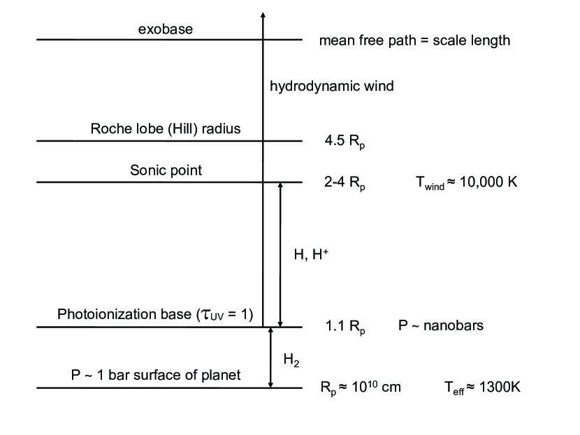
Figure 8.— Summary of important scales in our wind solutions. For a planet with properties inspired by HD 209458b, the $\tau=1$ surface to which UV photons penetrate is located where the local pressure is measured in nanobars, at about 1.1 times the radius of the 1 bar surface. Below this photoionization base, the temperature is $\sim$$10^{3}$ K, close to the effective temperature, as befits an atmosphere in radiative equilibrium with the incident stellar optical radiation balancing the planet’s thermal emission. Molecular chemistry (which we do not model) is important in this regime. Our model is valid above the $\tau=1$ surface, where the temperature is thermostated to $\sim$$10^{4}$ K by Lyman-$\alpha$ cooling. We demonstrate in Appendix A that our standard wind solution is insensitive to conditions below the $\tau=1$ surface, justifying our simple model which treats only atomic and ionized hydrogen. The sonic point of our wind solutions lies at 2–4 planetary radii, with smaller sonic point distances corresponding to higher UV fluxes. The Roche lobe radius of the planet at $\sim$$4.5R_{\rm p}$ is close enough to the sonic point radius that tidal gravity is significant. Below the exobase, where the mean free path to collisions equals the scale height of the atmosphere, the gas behaves as a fluid. Because the exobase is well outside the sonic point of our winds, mass loss from hot Jupiters takes the form of a hydrodynamic wind rather than Jeans escape.

3.2. Energy-Limited vs. Radiation/Recombination-Limited

The two regimes for mass loss that our numerical solution uncovered—$\dot{M}\propto F_{\rm UV}^{0.9}$ at low $F_{\rm UV}$ and $\dot{M}\propto F_{\rm UV}^{0.6}$ at high $F_{\rm UV}$ (Figure 7)—can be understood simply.

At low $F_{\rm UV}$, the flow is largely “energy-limited.” Most of the energy deposited by photoionizations as heat—i.e., $\sim$$\varepsilon\pi F_{\rm UV}R_{\rm p}^{2}$—goes into $PdV$ work, with little loss to radiation and internal energy changes (the relative contributions to the energy budget are given in §2.3.1). The $PdV$ work lifts material out of the planet’s gravitational potential well: measured per unit mass, the work done is

$$\frac{P\Delta V}{\rho R_{\rm p}^{2}H}\sim\frac{PR_{\rm p}^{3}}{\rho R_{\rm p}^{2}H}\sim\frac{\rho gHR_{\rm p}^{3}}{\rho R_{\rm p}^{2}H}\sim\frac{GM_{\rm p}}{R_{\rm p}}\,.$$

Then the energy-limited mass loss rate is given by

$$\dot{M}_{\rm e-lim} \sim \frac{\varepsilon\pi F_{\rm UV}R_{\rm p}^{2}}{GM_{\rm p}/R_{\rm p}}$$ (19)

$$\sim 6\times 10^{9}\left(\frac{\varepsilon}{0.3}\right)\left(\frac{R_{\rm p}}{10^{10}{\rm\,cm}}\right)^{3}\left(\frac{0.7M_{\rm J}}{M_{\rm p}}\right)$$

$$\left(\frac{F_{\rm UV}}{450{\rm\,erg}{\rm\,cm}^{-2}{\rm\,s}^{-1}}\right){\rm\,g}{\rm\,s}^{-1}\,,$$

close to the result found numerically at low $F_{\rm UV}$ (the factor of 5 difference in normalization between Equation 19 and the curve shown in Figure 7 arises mostly because the latter takes the substellar UV flux and applies it over all $4\pi$ steradians, whereas the former averages the UV flux over the surface of the planet—hence the factor of $\pi$ in equation 19). Energy-limited outflows were also found by Watson et al. (1981) who studied mass loss in the highly conductive atmospheres of the terrestrial planets.

At high $F_{\rm UV}$, the flow is “radiation/recombination-limited.” As quantified in §2.3.2, the input UV power is largely lost to cooling radiation. Radiative losses thermostat the gas temperature to $T\sim 10^{4}{\rm\,K}$. Under the approximation that the wind is isothermal, $\dot{M}\sim 4\pi\rho_{\rm s}c_{\rm s}r_{\rm s}^{2}$ at the sonic point, where $c_{\rm s}=[kT/(m_{\rm H}/2)]^{1/2}$ is the isothermal sound speed (the factor of 2 accounts for the fact that the hydrogen is nearly completely ionized), $r_{\rm s}=GM_{\rm p}/(2c_{\rm s}^{2})$, and $\rho_{\rm s}$ is the sonic point density. Between the $\tau=1$ surface and the sonic point, the density structure is nearly hydrostatic, so that

$$\rho_{\rm s}\sim\rho_{\rm base}\exp\left[\frac{GM_{\rm p}}{R_{\rm p}c_{\rm s}^{2}}\left(\frac{R_{\rm p}}{r_{\rm s}}-1\right)\right]\,.$$

In the high flux case, the density $\rho_{\rm base}$ at the $\tau=1$ photoionization base is $n_{+,{\rm base}}m_{\rm H}$. That density is determined by ionization equilibrium, which involves a balance between photoionizations and radiative recombinations (Figure 6):

$$\frac{F_{\rm UV}}{h\nu_{0}}\sigma_{\nu_{0}}n_{0,{\rm base}}\sim n_{+,{\rm base}}^{2}\alpha_{\rm rec}\,,$$

neglecting the order unity flux attenuation at the $\tau=1$ surface. The base neutral density $n_{0,{\rm base}}\sim 1/(\sigma_{\nu_{0}}H_{\rm base})\sim m_{\rm H}g/(2\sigma_{\nu_{0}}kT)$. This neutral density is fairly insensitive to $F_{\rm UV}$ (see beginning of §2 and compare Figures 2 and 5), and so we conclude that the radiation/recombination-limited mass loss rate is given by

$$\dot{M}_{\rm rr-lim}\sim 4\times 10^{12}\left(\frac{F_{\rm UV}}{5\times 10^{5}{\rm\,erg}{\rm\,cm}^{-2}{\rm\,s}^{-1}}\right)^{1/2}{\rm\,g}{\rm\,s}^{-1}\,,$$ (20)

similar to the answer found numerically at high $F_{\rm UV}$.

3.3. Spherical Asymmetry: Day/Night and Tidal Gravity

The mass loss rates given in all our plots are upper limits because they take our 1D solution for the substellar streamline and apply it over $4\pi$ steradians. The mass flux is maximized for the substellar streamline because the substellar point receives the maximal UV flux, and because the tidal gravity term weakens the planet’s gravity most along the line joining the planet to the star. We now discuss the extent to which the actual mass loss rate is reduced because of day/night differences in the received UV flux, and because of the directional dependence of tidal gravity. For simplicity we discuss these effects separately, as if they could be isolated from one another.

Ignoring for the moment differences between day/night external boundary conditions—these are actually significant and dealt with in §3.4—day/night differences would be erased in the extreme case that horizontal winds redistribute photoionized plasma from the dayside of the planet to the nightside, on a timescale shorter than the wind’s radial advection time of a few hours. In this case, the “nightside wind” would blow just as strongly as the “dayside wind.” In reality, if the dayside wind blows freely (see §3.4 for important reasons to believe that it may not), the timescale for horizontal advection is at least as long as that for radial advection, since the distances travelled in both cases are several $R_{\rm p}$, the radial speed is supersonic, and the horizontal speed is at most sonic. So if the dayside wind blows, the nightside wind is likely muted. The inverse is also true—see §3.4.

In the opposite limit of no horizontal redistribution, the mass loss rates we have calculated would be reduced by a factor of $(1/2)\int_{0}^{\pi/2}\sin\theta(\cos\theta)^{\gamma}d\theta=1/[2(\gamma+1)]$, where $\theta$ is the angle measured from the substellar ray ($\theta=0$ points along the substellar ray, while $\theta=\pi/2$ defines the terminator dividing day from night), and the $(\cos\theta)^{\gamma}$ factor accounts for how the planetary mass flux scales with incident stellar flux (which itself scales as $\cos\theta$). For energy-limited flows, $\gamma=0.9$, and for radiation/recombination-limited flows, $\gamma=0.6$ (see Figure 7). The reduction factor equals 1/3.8 = 0.26 and 1/3.2 = 0.31 in the two respective cases. If there is horizontal redistribution, we do not expect the reduction factors to change appreciably from these values. To first order, redistribution of plasma simply redistributes the wind over the planetary surface. Changes in the total mass loss rate are expected to be of second order. For example, if the wind is strictly energy-limited (§3.2), the mass loss rate depends only on the amount of UV radiation intercepted by the planet, and is independent of the degree of redistribution.

To get a sense of how much the mass loss rate is reduced because tidal gravity does not point parallel to all streamlines emanating from the planet, we eliminate the tidal term from the force equation (2) and re-solve the fluid equations. We obtain a mass loss rate (multiplying by $4\pi$ steradians) that is 0.79 $\times$ our standard model result. This can be considered a maximum reduction factor for the directional dependence of tidal gravity insofar as its effect can be isolated.

Though tidal gravity does not change the calculated mass loss rate appreciably, it is nonetheless important for two reasons. First, tidal gravity alters the velocity structure of the wind, allowing it to accelerate to larger speeds (Figure 9). Second, tidal gravity moves the location of the sonic point to lower altitude, allowing it to remain within the Roche lobe along the substellar ray and helping validate our 1D treatment.

Figure 9.— Wind velocity as a function of altitude for our standard model with tidal gravity (solid curve) and without (dashed curve). Tidal gravity alters the velocity profile of the wind, allowing the flow to attain higher speeds. It also moves the wind’s sonic point to lower altitude.

To summarize this subsection, if the dayside transonic wind blows freely, our crude accounting for the directional dependences of UV irradiance and of tidal gravity suggest that actual mass loss rates are lower than our plotted values by factors of $\sim$4. We now turn to the question of whether the dayside wind can actually blow, when faced with the considerable pressure of the host star wind.

3.4. Colliding Winds and Breezes: Trading the Dayside Wind for the Nightside Wind

The planetary wind does not exist in vacuum. The dayside wind blows into the plasma streaming from the star: the stellar wind. Stellar and planetary winds collide and mix in a standing bow shock surrounding the planet. The situation is analogous to the colliding winds of massive stellar binaries (Luo et al., 1990; Stevens et al., 1992). Figure 10 supplies a cartoon illustration. However, as stressed in the figure caption and in the discussion below, numerous assumptions underlie this cartoon, and reality is likely to look substantially more complicated.

Figure 10.— Cartoon of the standing bow shock (heavy curve) where planetary and stellar winds collide and mix. For this figure only, in order to compute the location of the bow shock, we assume for simplicity that the winds are spherically symmetric, have zero thermal and magnetic pressure, and have constant velocity (we neglect Coriolis, centrifugal, and gravitational forces—we have not directly used one of our wind models). For the stellar wind, we assume a mass loss rate of $5\times 10^{11}{\rm\,g}{\rm\,s}^{-1}$ and a velocity of 400 km/s. For the planetary wind, we take $3\times 10^{10}{\rm\,g}{\rm\,s}^{-1}$ and 20 km/s, values informed by our wind models. The bow shock is given by the condition that the bulk momentum fluxes (“ram” pressures) normal to the shock balance (e.g., Luo et al., 1990). Such a shock does not influence the planetary wind upstream if it is located outside the sonic radius, as is drawn. In reality, this condition may not be satisfied because of the overwhelming total pressure of the stellar wind.

At the stand-off shock, the total pressures of the two flows balance. The total pressures include contributions from “ram” ($\rho v^{2}$), thermal, and magnetic pressure, but should include only components that are normal to the shock front (the shocks are oblique). The total pressure of the planetary wind decreases monotonically with distance from the planet. If the total stellar wind pressure $P_{\ast,{\rm tot}}$ near the planet is less than the total planetary wind pressure $P_{\rm tot}(r_{\rm s})$ at the planetary wind’s sonic point, then the stand-off shock will be located downstream of the planet’s sonic point. There it cannot influence the planetary flow upstream, for the same reason that one cannot shout upstream in a supersonic flow and be heard. In this case the transonic wind solution that we have obtained for $r<r_{\rm s}$—and in particular our computed mass flux—would remain unchanged.

What are $P_{\ast,{\rm tot}}$ and $P_{\rm tot}(r_{\rm s})$ for a hot Jupiter orbiting a main-sequence, solar type star? For the former quantity we are guided by observations of the solar wind. At $a=0.05{\rm\,AU}=10R_{\odot}$, the solar wind has accelerated to nearly its maximum speed (McKenzie et al., 1997; Marsch et al., 2003). Approximating the stellar wind velocity as constant from 0.05 to 1 AU, we scale characteristic spacecraft measurements (SOHO; Ulysses) of the solar wind density and velocity at 1 AU to estimate the corresponding density $n_{\ast}$ and velocity $v_{\ast}$ at 0.05 AU: $n_{\ast}\sim 6(1/0.05)^{2}\,{\rm protons}{\rm\,cm}^{-3}$ and $v_{\ast}\sim 400{\rm\,km}{\rm\,s}^{-1}$. We take the local proton temperature to be $T_{\ast}\sim 10^{6}{\rm\,K}$ (the electron temperature is several times lower; McKenzie et al. 1997), and the magnetic field strength to be $B_{\ast}\sim 0.01$ G at 10 stellar radii (Banaszkiewicz et al., 1998). Then $P_{\ast,{\rm tot}}\sim n_{\ast}m_{\rm H}v_{\ast}^{2}+n_{\ast}kT_{\ast}+B_{\ast}^{2}/(8\pi)\sim 10$ picobars, with the ram and magnetic pressures dominating. This is an overestimate insofar as we are not taking the components of the ram and magnetic pressures that are relevant perpendicular to the shock front. Compare this to $P_{\rm tot}(r_{\rm s})\sim 3$ pbars, as calculated for our standard model of the substellar streamline (see Figure 11), neglecting the unknown magnetization of the planet. Given the uncertainties, the most we can say is that $P_{\ast,{\rm tot}}$ and $P_{\rm tot}(r_{\rm s})$ are comparable. While a transonic wind solution along certain (not necessarily substellar) streamlines may yet be possible, it is also possible—indeed even likely, given the fact that the solar wind can gust to values of $n_{\ast}$ and $v_{\ast}$ several times higher than the ones we have used—that the stellar wind squashes the planetary dayside outflow down to a subsonic breeze, or even stops dayside photoevaporative mass loss completely.

A breeze would still blow a bubble in the stellar wind, like that drawn in Figure 10, only smaller. But because a breeze is subsonic, it would not traverse a shock at the bubble boundary. Unlike the case for the supersonic wind, a breeze is in causal contact with the flow at the boundary; i.e., conditions at the boundary influence, via sound waves, conditions in the interior. The radial velocity would decrease smoothly to zero at the bubble boundary, giving rise to large pressure gradients that would drive flows parallel to the boundary (by analogy to subsonic flow around a blunt obstacle such as a hard sphere). The flow inside the bubble would be nonradial and multidimensional. Unfortunately, we cannot easily capture such behavior with our 1D model; if we tried to model a breeze by imposing a boundary condition of zero radial velocity at finite distance from the planet, while insisting simultaneously on a non-zero mass loss rate, our simple continuity relation (1) would yield infinite density.

Nevertheless, we can get a sense of how much the dayside mass loss rate might be reduced in the presence of external pressure, by re-running our relaxation code with boundary condition (15) replaced by $[v^{2}=\beta\gamma kT/\mu]_{r_{\rm s}}$, where $\beta<1$ is our breeze parameter. Note that $r_{\rm s}$ in this case is no longer the sonic point but is instead the location where the flow stops accelerating and starts decelerating. Resulting breeze solutions are shown in Figure 11, with the corresponding mass loss rates plotted in Figure 12. While the total pressure $P_{\rm tot}$ for the $\beta=1$ wind solution decreases to zero at large distance, $P_{\rm tot}$ for a $\beta<1$ breeze asymptotes to a finite value. As $\beta$ decreases, the breezes blow more slowly, approaching the $v=0$ limiting solution for a hydrostatic atmosphere. Once $\beta\lesssim 10^{-2}$ ($v\lesssim 0.1\sqrt{\gamma kT/\mu}$), the $P_{\rm tot}$ profiles hardly change. We take as a reference pressure $P_{{\rm tot}}(r_{\rm s})$; the location $r_{\rm s}$ is a sensible one to examine since for the most part it decreases as $\beta$ decreases, mimicking the shrinking of the planetary bubble with stronger stellar winds. Over the entire family of breezes, the reference pressure $P_{\rm tot}(r_{\rm s})$ achieves a maximum value of $\sim$40 pbar for our standard parameters and boundary conditions. (Recall that an isothermal hydrostatic atmosphere has a finite pressure at infinity.)

To the extent that our 1D solution lends insight into the 3D breeze problem, we conclude the following: if the stellar wind pressure $P_{\ast,{\rm tot}}\lesssim 3$ pbars, the planet emits a full-fledged transonic wind; if $P_{\ast,{\rm tot}}$ lies between $\sim$3 and $\sim$40 pbars, then the planet emits a dayside breeze with a finite mass loss rate; but if $P_{\ast,{\rm tot}}\gtrsim 40$ pbars, then the planet’s dayside atmosphere is forced to be radially hydrostatic, with the stellar wind penetrating to the depth where pressure balance is achieved. Figure 12 informs us that tiny increases in $P_{\rm tot}(r_{\rm s})$ above 35 pbars correspond to enormous reductions in $\dot{M}$. At the same, if $P_{\rm tot}(r_{\rm s})$ is below 35 pbar, the mass loss rate is $\sim$$10^{10}{\rm\,g}{\rm\,s}^{-1}$, to within a factor of about 3. Thus, the stellar wind can act essentially as an on-off switch—at times permitting the planet to lose mass from its dayside at near maximum rates of order $10^{10}{\rm\,g}{\rm\,s}^{-1}$, and at others shutting down dayside mass loss completely. In the case of hot Jupiters orbiting main-sequence stars, given how the stellar outflow pressure is of order 10 pbar and how it may increase dramatically during violent coronal mass ejections, we expect this switch to flip back and forth with stellar activity. We cannot rule out the possibility that the dayside switch might even be off the majority of the time.

Figure 11.— Velocity and total pressure ($P_{\rm tot}=\rho v^{2}+P$) profiles for our unique transonic wind ($\beta=1$) and a family of breezes ($\beta<1$ as labelled), for standard model parameters. The x symbol marks $r=r_{\rm s}$, which for the wind represents the sonic point, and for breezes represents the point of maximum velocity. At infinity, breezes remain pressurized while the wind does not. In the middle panel, profiles not labelled include $\beta=10^{-2}$, $10^{-3}$, and $10^{-4}$. Note how these profiles hardly change as $\beta$ decreases—the solution is approaching that of a $v=0$ hydrostatic atmosphere. The bottom panel shows that for the wind, thermal pressure dominates at depth (dotted line), while $\rho v^{2}$ “ram” pressure dominates at altitude (dashed line). For the $\beta=0.01$ breeze shown, thermal pressure dominates everywhere. For the most part, $r_{\rm s}$ shrinks as ever slower breezes (smaller $\beta$) are considered. The exception occurs for $\beta\lesssim 10^{-2}$ (middle panel), and is an artifact of our choice to compute $\tau(r_{\rm s})$ out to the fixed Roche lobe radius $R_{\rm Roche}$; $\tau(r_{\rm s})$ increases with decreasing $\beta\lesssim 10^{-2}$.

Figure 12.— Mass loss rates (assuming $4\pi$ symmetry) for our breeze solutions. Mass loss rates become arbitrarily small as the breeze parameter $\beta$—which sets the maximum breeze velocity at $r_{\rm s}$—decreases. Interestingly, the total pressure $P_{\rm tot}(r_{\rm s})$ asymptotes to a maximum value of $\sim$40 pbar as ever slower breezes are considered (see also Figure 11). The existence of a maximum pressure suggests that if the stellar wind exerts an external pressure in excess of $\sim$40 pbar (for our standard parameters and boundary conditions), it will shut down the dayside planetary outflow completely.

Even when the dayside switch is off, however, we do not expect mass loss to shut down completely. As the dayside outflow weakens, the nightside wind should strengthen in proportion. That is because the UV energy that the planet absorbs must be spent one way or another; if it is prevented from doing $PdV$ work against gravity on the dayside, it will instead power horizontal winds which carry heat to the nightside. Shielded from the stellar wind, the nightside is free to emit its own wind. Thus, the total mass loss rate might remain roughly constant at $\sim$$10^{10}{\rm\,g}{\rm\,s}^{-1}$, even when the stellar wind gusts (assuming that no other energy sink becomes active).

In concluding that nightside winds will blow when dayside mass loss has been quenched, we have implicitly assumed that the planet resides outside of the region where the dipolar component of the star’s magnetic field dominates. Inside this region—i.e., inside the star’s Alfvén radius—most magnetic field lines are not blown open by the stellar wind. Closed, poloidal field lines can encage both dayside and nightside winds, confining atmospheric escape to magnetic flux tubes in the vicinity of the planet’s poles. The detailed structure of the solar magnetosphere has not been conclusively established. Some models (e.g., McKenzie et al., 1997; Marsch et al., 2003) place the solar Alfvén radius near 10 $R_{\odot}$, near the orbit of a hot Jupiter. However, the three-dimensional model of Banaszkiewicz et al. (1998, their “DQCS” model with Q = 1.5) states that at $10R_{\odot}$, field lines are primarily radial, and by implication, the Alfvén surface lies at smaller radius.

What about for hot Jupiters orbiting T Tauri stars? To what extent are their dayside outflows squashed by the highly pressurized winds emitted by young active stars? If magnetospheric truncation of T Tauri accretion disks sets the final orbits of inwardly migrating hot Jupiters (Lin et al., 1996), these planets likely also reside near the Alfvén radii of their host star magnetospheres, where the stellar ram and magnetic pressures are comparable. This conclusion is compatible with observations of mass loss rates from T Tauri stars in the range $10^{-9}$ to $10^{-7}M_{\sun}/$yr (Edwards et al., 1987) and T Tauri surface fields that are $10^{3}$ times stronger than their main-sequence counterparts (e.g., Johns-Krull et al., 1999). We therefore estimate that $P_{\ast,{\rm tot}}\sim 10\times(10^{3})^{2}$ pbar $\sim 10$ $\mu$bar. Let us compare this pressure to the pressures characterizing planetary outflows. Figure 13 shows a family of breeze solutions for a T Tauri-like UV flux of $F_{\rm UV}=5\times 10^{5}{\rm\,erg}{\rm\,cm}^{-2}{\rm\,s}^{-1}$. It shows that $\max(P_{{\rm tot}}(r_{\rm s}))\approx 4$ nanobar $\ll P_{\ast,{\rm tot}}$. Thus, it seems safe to conclude that T Tauri stellar winds completely stifle dayside winds from hot Jupiters.

It is not clear whether hot Jupiters around T Tauri stars reside inside or outside their host stars’ Alfvén radii. If stellar rotation rates are locked to disk rotation rates at Alfvén radii (“disk locking”; e.g., Herbst & Mundt 2005), this question reduces to whether the planet orbits inside or outside the corotation circle. The current measured rotation period of HD 209458 of $\sim$12.4 days (Winn et al., 2005, and references therein) yields a corotation radius of $\sim$0.1 AU. However, T Tauri stars typically rotate faster than their main-sequence counterparts (e.g., Hartmann et al., 1986; Johns-Krull & Gafford, 2002). Furthermore, observations of T Tauri magnetic fields do not consistently confirm models in which the closed field extends to the corotation radius (Jardine et al., 2008, and references therein).

Given these uncertainties, we acknowledge two possibilities. Winds from giant planets located well inside the magnetospheres of their T Tauri host stars will be confined on both day and night sides by magnetic pressure, blowing only along polar flux tubes. Hot Jupiters located in open field line regions experience quenching only on the day side—they lose mass strictly by night.

Figure 13.— Same as Figure 11, but for the high flux case where $F_{\rm UV}=5\times 10^{5}{\rm\,erg}{\rm\,cm}^{-2}{\rm\,s}^{-1}$. Over all wind and breeze solutions, the reference pressure $P_{\rm tot}(r_{\rm s})$ does not exceed $\sim$4000 pbar (middle panel). Since T Tauri stellar wind pressures are about three orders of magnitude greater than this (see text), we expect the daysides of hot Jupiters orbiting pre-main-sequence stars to emit neither winds nor breezes, but to have radially hydrostatic atmospheres. Their nightsides, however, may well be losing mass at a rate of order $10^{12}{\rm\,g}{\rm\,s}^{-1}$, since we expect horizontal winds to carry hot photoionized plasma from the dayside to the nightside.

3.5. Radiation Pressure

Can stellar radiation pressure drive substantial planetary mass loss? Neutral H atoms absorbing stellar Ly$\alpha$ photons feel a radiation pressure force $F_{{\rm Ly}\alpha}\sigma_{{\rm Ly}\alpha}/c$, where $c$ is the speed of light. We use the solar Ly$\alpha$ flux scaled to $a=0.05{\rm\,AU}$, $F_{{\rm Ly}\alpha}\sim 2.4\times 10^{3}$erg/cm²/s (Woods et al., 2000). If the line were only thermally broadened with a velocity of $\sim$$10{\rm\,km}{\rm\,s}^{-1}$, the absorption cross section at line center would be $\sigma_{{\rm Ly}\alpha}\sim 6\times 10^{-14}{\rm\,cm}^{2}$. To account for extra Doppler broadening from a range of bulk velocities extending up to $v_{\rm orb}$, we lower the thermally broadened cross section by another factor of 10: $\sigma_{{\rm Ly}\alpha}\sim 6\times 10^{-15}{\rm\,cm}^{2}$. Putting it all together, we find that the radiation pressure force is comparable to that of stellar gravity, $GM_{\ast}m_{\rm H}/a^{2}$, in agreement with the result of Vidal-Madjar et al. (2003). But, radiation pressure of this magnitude would require of order an orbital period (days) to accelerate H atoms to velocities of $v_{\rm orb}\sim 100{\rm\,km}{\rm\,s}^{-1}$. The observations, in contrast, require this acceleration to occur over a few hours, the time to travel $\sim$$10R_{\rm p}$, the size scale probed by the transit. Furthermore, atoms are subject to Ly$\alpha$ radiation pressure for only several hours before they are photoionized. These considerations imply that a larger Ly$\alpha$ flux than we have assumed would be required to accelerate neutral hydrogen to $\sim$100 km/s (Holmström et al., 2008).

Nonetheless, we assume optimistically that radiation pressure can in fact accelerate H atoms to $\sim$$v_{\rm orb}$ and estimate the resultant mass loss rate. Radiation pressure can only act on gas that is optically thin to Ly$\alpha$ photons. The column density to optical depth unity is $N_{{\rm Ly}\alpha}=1/\sigma_{{\rm Ly}\alpha}\sim 2\times 10^{14}{\rm\,cm}^{-2}$. Hydrogen is accelerated off the planet’s limb; the area of the annulus presented by hydrogen within the planet’s Roche lobe is $\sim$$R_{\rm Roche}^{2}$. This hydrogen is removed every $R_{\rm Roche}/v_{\rm orb}$ time. Putting it all together, we estimate a mass loss rate due to radiation pressure of

$$\dot{M}_{\rm rad.press.}\sim\frac{N_{{\rm Ly}\alpha}R_{\rm Roche}^{2}m_{\rm H}}{R_{\rm Roche}/v_{\rm orb}}\sim 10^{8}{\rm\,g}{\rm\,s}^{-1}\,,$$ (21)

two orders of magnitude lower than the mass loss rates we have computed for photoionization-heated, hydrodynamic winds. We conclude that radiation pressure is not a significant driver of planetary outflows when compared against photoionization.

Vidal-Madjar et al. (2003) claim a mass loss rate of $10^{10}{\rm\,g}{\rm\,s}^{-1}$ based on line-driven acceleration to large blue-shifted velocities of gas that has been raised, presumably by other means, to the altitude of the Roche lobe. Their claim is based in part on an assumed hydrogen density of $n_{0}\sim 2\times 10^{5}{\rm\,cm}^{-3}$ at a distance of $r=R_{\rm Roche}/2$. But the corresponding column $n_{0}R_{\rm Roche}/2\sim 4\times 10^{15}\gg N_{{\rm Ly}\alpha}$ would be optically thick to Ly$\alpha$ photons ($\tau_{{\rm Ly}\alpha}\sim 20$).

4. SUMMARY AND COMPARISON WITH OBSERVATIONS

We have presented a simple model of atmospheric escape from hot Jupiters, as driven by photoionization heating by stellar UV radiation. To calculate the steady-state structure of the planetary wind, we employed a relaxation code to solve the equations of ionization balance and of mass, momentum, and energy conservation. We imposed two-point boundary conditions that allowed us to find the unique wind solution that transitions from subsonic to supersonic velocities. Tidal gravity is important to include in our momentum equation because it alters the entire velocity structure of the wind, generating higher velocities and helping to lower the wind’s sonic point to within the Roche lobe, at least for the substellar streamline. Photoionization heating is balanced by a combination of $PdV$ work and cooling by Lyman-$\alpha$ radiation. The latter serves as a thermostat, limiting planetary wind temperatures to $\sim$$10^{4}$ K over four decades in incident UV flux. Notably, conductive transport of energy is not important, by contrast to the thermospheres of terrestrial planets.

Our assumption that mass loss from hot Jupiters takes the form of hydrodynamic winds rather than local Jeans escape is self-consistent: in our solution, escaping gas remains collisional at the sonic point. Showing that this condition is satisfied at the sonic point is sufficient because the flow inside the sonic point is denser and hence still more collisional, while the flow outside the sonic point is supersonic and so cannot influence the flow inside—in a supersonic flow, one cannot shout upstream and be heard. We agree with Tian et al. (2005) and García Muñoz (2007) that the flow is never in a regime where Jeans escape considerations are relevant (see §3.1).

We find that a planet similar to the transiting hot Jupiter HD 209458b loses mass at a maximum rate of $\sim$$10^{10}{\rm\,g}{\rm\,s}^{-1}$ for a UV flux characteristic of low to moderate solar activity. For a UV flux near the Lyman edge that is $\sim$2–3 times larger, as obtains during solar maximum (Woods et al., 2005; Lean et al., 2003, and references therein), the mass loss rate is $\sim$$2\times 10^{10}{\rm\,g}{\rm\,s}^{-1}$ (we have shown that at these fluxes, mass loss is energy-limited and scales nearly linearly with UV flux). This maximum mass loss rate is two orders of magnitude lower than the $10^{12}\,{\rm g/s}$ quoted by Lammer et al. (2003), and inconsistent with the claim by Baraffe et al. (2004) that planets lighter than 1.5 Jupiter masses at 0.05 AU from their stars evaporate entirely in $<5$ Gyr. We agree with Tian et al. (2005) (who idealize the wind as neutral), Yelle (2006), and García Muñoz (2007) that the current mass loss rate from HD 209458b causes the planet to lose at most 1% of its mass over its 5 Gyr age.

What explains the factor of 100 discrepancy between our maximum mass loss rates and the mass loss rates given by Lammer et al. (2003) and Baraffe et al. (2004)? These authors, inspired by Watson et al. (1981) who model mass loss from the highly conductive atmospheres of terrestrial planets, posit that outflows from hot Jupiters are energy-limited. Energy-limited flows are those for which a fixed fraction of the stellar UV radiation incident upon a planet’s surface goes towards driving gas out of the planet’s gravitational well. As we have shown, conduction is not important in the winds emitted by hot Jupiters, and therefore the details of the calculation by Watson et al. (1981) are not transferable. Nonetheless, we find that for $F_{\rm UV}\lesssim 10^{4}{\rm\,erg}{\rm\,cm}^{-2}{\rm\,s}^{-1}$, as obtains for hot Jupiters orbiting main-sequence solar analogs, hot Jupiter winds are indeed nearly energy-limited. The energy-limited mass loss rate can be written as

$$\dot{M}_{\rm lim}\approx\frac{\varepsilon F_{\rm UV}\times\pi r_{1}^{2}}{GM_{\rm p}/r_{0}}$$ (22)

(Watson et al., 1981, see also our Equation 19), where gas is bound to the planet below radius $r_{0}$ and the bulk of incoming UV radiation is absorbed at $r_{1}$. The difference between our calculated $\dot{M}$ and that derived by Lammer et al. (2003) arises from two factors. First, we include a heating efficiency $\varepsilon<1$, which must account at least for the energy lost to photoionizing atoms. In our simple model, $\varepsilon\approx 0.3$ (recall Equation 4). Second, and more significantly, our calculation places $r_{0}$ and $r_{1}$ closer to $1.1R_{\rm p}$ (see beginning of §2), the location of the $\tau=1$ surface to photoionization. Lammer et al. (2003) take instead $r_{0}\approx r_{1}\approx 3R_{\rm p}$ by applying detailed formulae derived by Watson et al. (1981). These formulae are not appropriately applied to the photoionized upper atmospheres of hot Jupiters, because in these environments conductive cooling is not significant. García Muñoz (2007) reaches essentially the same conclusion; see his section 3.5.

For high UV fluxes $\gtrsim 10^{4}{\rm\,erg}{\rm\,cm}^{-2}{\rm\,s}^{-1}$, like those incident upon hot Jupiters orbiting active T Tauri stars, mass loss ceases to be energy-limited. Most of a fast photoelectron’s energy is lost to collisionally excited Ly$\alpha$ radiation. By contrast to the case at low $F_{\rm UV}$ where photoionizations are balanced by gas advection and the neutral gas fraction remains of order unity at altitude, at high $F_{\rm UV}$ photoionizations are balanced by radiative recombinations. The transition to a nearly completely ionized flow is sharp, and the overall wind structure is reminiscent of a classic expanding H II region. Whereas in the energy-limited regime $\dot{M}$ is expected to scale as $F_{\rm UV}^{1}$, in the radiation/recombination-limited regime $\dot{M}$ is expected to scale as $F_{\rm UV}^{1/2}$, essentially because that is how the number density of ionized atoms scales in a plane-parallel Strömgren slab. Our detailed numerical model yields power-law indices of 0.9 and 0.6 at low and high UV flux, respectively.

We have demonstrated that above the $\tau=1$ surface to photoionization, our wind model is insensitive to our chosen boundary conditions. This helps to justify our neglect of hydrogen molecular chemistry. The uncertainty generated by this omission is embodied in our choice of the base radius $r_{\rm min}$, which by definition is that radius where hydrogen is predominantly atomic. Without modelling the chemistry of H₂, we cannot be sure where $r_{\rm min}$ is located. But we have shown that we can estimate it to sufficient accuracy (about 10%; see the order-of-magnitude discussion at the beginning of §2) that our mass loss rates are uncertain by at most factors of a few (see Figure 24 of Appendix A). The bulk properties of our wind solutions are in good agreement with those of García Muñoz (2007) and our ionization profiles agree well with those of Yelle (2004). Both García Muñoz (2007) and Yelle (2004) model hydrogen and helium molecular chemistry in hot Jupiter winds, and García Muñoz (2007) includes contributions from D, C, N, O, and CH. García Muñoz (2007) finds that if metals are present in the wind in solar abundances, they can increase the mass loss rate by factors of a few by reducing the effectiveness of H${}_{3}^{+}$ cooling at depth (below the $\tau=1$ surface to photoionization). Again, these details can be considered buried in our parameter $r_{\rm min}$.

Neither Yelle (2004) nor García Muñoz (2007) considered the effects of Lyman-$\alpha$ line cooling—which we have demonstrated is important for large UV fluxes—or of line cooling from metals such as O II, O III, and N II. If classic H II regions are any guide, metal line cooling could exceed Ly$\alpha$ cooling, lowering hot Jupiter wind temperatures by up to a factor of 2 (Osterbrock, 1989). Metal abundances in the upper thermosphere are extremely uncertain, depending on unknown turbulent mixing coefficients (“eddy diffusivities”). In any case, we do not expect metal line cooling to change our results qualitatively. It can only lower mass loss rates and wind velocities somewhat, strengthening our main conclusions.

It is often said that transonic winds are characterized by zero pressure at infinite distance, while subsonic breezes have finite pressure at infinity (e.g., García Muñoz, 2007). But in practice, when considering how the outflow from the planet’s dayside interacts with the outflow from its host star, whether the dayside emits a wind or a breeze does not require us to examine conditions at infinity. Rather, we evaluate conditions at the sonic point. Again, as with our criterion for hydrodynamic escape, the sonic point serves as discriminant because once the flow achieves supersonic velocities past the sonic point, it cannot influence the flow inside the sonic point. If the total external pressure (ram, thermal, and magnetic) exerted by the host star’s wind is less than the total pressure exerted by the transonic planetary wind at its sonic point, then the transonic wind solution obtains. Otherwise, either the dayside emits a more gentle breeze or—if the external pressure exceeds some critical value—the dayside atmosphere does not escape at all but is forced to be in vertical hydrostatic equilibrium. To the extent that the host star of HD 209458b emits a highly variable wind like that of the Sun, we find that the stellar wind pressure is comparable to the planetary wind pressure at the sonic point (both are measured in tens of picobars). During violent coronal mass ejections, the stellar wind pressure may overwhelm the planetary wind pressure. Thus we expect that dayside winds from hot Jupiters orbiting main-sequence solar type stars will alternately turn on and off (with a duty cycle that might well favor the off state). When the dayside wind is off, we expect the nightside wind to turn on and pick up the slack—the absorbed UV energy now being used to power horizontal flows that carry photoionized plasma to the planet’s nightside, which is shielded from the stellar wind and therefore immune to pressure confinement.

Winds from T Tauri stars have magnetic and ram pressures that are some six orders of magnitude greater than their main-sequence counterparts. Were a hot Jupiter orbiting a T Tauri star to also emit a wind, the pressure at its sonic point would be greater than under main-sequence conditions, but only by about three orders of magnitude according to our model. Thus, a T Tauri stellar wind will entirely quash dayside outflows from orbiting hot Jupiters. Outflows from the nightside (if the planet is outside the stellar Alfvén radius) or along polar field lines (if the planet is inside the Alfvén radius) would carry away at most $\sim$$2\times 10^{12}{\rm\,g}{\rm\,s}^{-1}\times 10^{7}{\rm\,yr}$ or $\sim$$6\times 10^{-4}$ of the planetary mass. These quantitative considerations rule out speculations that mass loss is significant during the host star’s youth (e.g., Baraffe et al., 2004).

Returning to the main-sequence case, to what degree will a hot Jupiter wind absorb stellar Ly$\alpha$ photons and produce an observable transit signature? Figure 14 shows, for standard model parameters, how the extinction varies with wavelength in the Ly$\alpha$ line, assuming the planet is in mid-transit and that its orbit is viewed edge on. The extinction is integrated across the entire stellar disk (to perform this integral, we extend our wind model out to $r=10R_{\rm p}\approx 2R_{\rm Roche}$). Local line profile functions are Voigt profiles, which include thermal and natural broadening. Out to Doppler shifts of $\pm 30{\rm\,km}{\rm\,s}^{-1}$, comparable to bulk wind velocities, the line is essentially black (the Ly$\alpha$ emission produced by the wind itself is negligible since densities are low enough that the $n=2$ population of neutral hydrogen is well below the LTE value). At Doppler shifts of $\pm 100{\rm\,km}{\rm\,s}^{-1}$, the extinction plummets to 2–3%. This result is at odds with the observational claim that HD 209458b reduces the stellar Ly$\alpha$ flux by some 9–15% at $\pm 100{\rm\,km}{\rm\,s}^{-1}$ while in transit (Vidal-Madjar et al., 2003; Ben-Jaffel, 2007; Vidal-Madjar et al., 2008).

Figure 14.— Maximum fraction of stellar Ly$\alpha$ radiation obscured by absorption in the planetary wind, plotted as a function of Doppler shifted velocity from line center. We apply our wind solution for the substellar streamline over all $4\pi$ steradians of the planet’s surface. We assume that the planet is located at mid-eclipse, and that its orbital inclination relative to the stellar equator is zero. For each projected distance from the planet’s center ranging from $R_{\rm p}$ to $8.2R_{\rm p}=R_{\ast}$, we calculate a line-of-sight optical depth, integrating up to a maximum altitude of $10R_{\rm p}$. We include both natural and thermal line broadening. The ordinate is the fraction of the stellar disk that is obscured, accounting only for $e^{-\tau}$ absorption and neglecting scattering and wind self-emission. All of our assumptions maximize the obscuration. Absorption drops sharply beyond a few tens of km/s to a constant of 1.5% (horizontal dashed line), the decrement in the visible continuum. The velocity scale of $\sim$20 km/s is set by thermal broadening ($\sim$$10$ km/s at $10^{4}{\rm\,K}$), together with the bulk velocity (10–30 km/s at Mach numbers of a few). If the wind is emitted only from the dayside (nightside), our extinction curve will be valid only at wavelengths redward (blueward) of line center. Absorption by the planetary wind does not account for the claimed $\sim$9–15% decrement in flux from HD 209458b at Doppler equivalent velocities near $\pm 100$ km/s, as integrated over the intervals between the two dotted lines and between the two dot-dashed lines (Vidal-Madjar et al., 2003; Ben-Jaffel, 2007). We further emphasize this inconsistency in Figure 15.

To drive this point home, we present in Figure 15 the predictions of our model for the Ly$\alpha$ line during transit, computed by combining the out-of-transit line spectrum from Vidal-Madjar et al. (2003, taken from their Figure 2) with our extinction curve (Figure 14). Over the wavelength intervals used by Vidal-Madjar et al. (2003), our model produces a flux decrement of 2.9%. Shown for comparison is the observed in-transit line spectrum from Vidal-Madjar et al. (2003). Agreement between model and observation is poor: the model spectrum is hardly absorbed at large velocities, by contrast to the observed spectrum.

Figure 15.— Observed out-of-transit (dashed line) and in-transit (dotted line) spectra, reproduced from Figure 2 of Vidal-Madjar et al. (2003). In the line “core” from -42 to +32 km/s, where interstellar absorption is strong, we set the flux to zero. Our theoretical in-transit spectrum (solid line) is computed by attenuating the observed out-of-transit spectrum according to our extinction curve in Figure 14. Theory predicts substantially less absorption than is claimed to be observed. However, the spectrally unresolved measurements of Vidal-Madjar et al. (2004), taken at a different epoch and in principle pertaining to much smaller Doppler equivalent velocities than were implicated by Vidal-Madjar et al. (2003), may well be due to the wind. Integrated over the line profile outside the core, our model predicts a flux decrement of 2.4%, close to that observed by Vidal-Madjar et al. (2004).

What could explain this discrepancy between our model and the observations? Three possibilities present themselves: (1) Our model underestimates the column of neutral hydrogen generated by the wind during transit by a factor of $\sim$3–5; (2) physics that is missing from our model generates a population of neutral hydrogen moving at velocities larger than the bulk velocity of the wind; or (3) the observed flux decrement at $\pm$100 km/s is due to some combination of geocoronal emission and intrinsic stellar variability (see also Ben-Jaffel 2007): processes that, if observed over long enough times, should not be correlated with the orbital phase of the planet. We now comment on possibilities (1) and (2).

Our wind model generates a Ly$\alpha$ flux decrement of $\sim$3% at Doppler-equivalent velocities of $\pm 100$km/s due to naturally broadened, Lorentzian line wings. If the column of neutral hydrogen traversed by stellar Ly$\alpha$ photons along lines of sight located 5–10$R_{\rm p}$ from the planet were larger by a factor of 3–5, then absorption generated by the line wings might generate the 9–15% absorption observed at $\pm 100$km/s. Ben-Jaffel (2008) argues that this is the case using the wind profiles of Garcia-Munoz (2007), who calculates that the wind is $\sim$30% neutral at $\sim$5$R_{\rm p}$. At these distances, we find a neutral fraction of $\sim$13% for our base case and $\sim$6% for parameters matching those used in Garcia-Munoz (2007), though in other respects our wind solutions largely agree. Our ionization profiles are in better agreement with the solutions of Yelle (2004), which do not generate sufficient absorption in the Lorentzian line wings to match observations (Ben-Jaffel 2008). The reason for these differences merits further attention. As previously noted, 1D wind solutions such as those in this paper, Yelle (2004), and Garcia Munoz (2007) break down at planetocentric distances greater than $\sim$5–10$R_{\rm p}$. Multidimensional calculations could yield a larger neutral column (J. Stone, personal communication).

Alternatively, is there some qualitative physics that our model is missing that could generate a population of neutral H atoms moving at velocities of $\sim$100 km/s? An appeal might be made to interaction of the planetary wind with the stellar wind: in the bow shock, neutral hydrogen from the planet mixes with fast moving stellar plasma and might be accelerated to large blueshifted velocities (see the simulations by Stevens et al. 1992 of colliding stellar winds). But no similar argument can be made for the observed redshifted absorption—which, according to Ben-Jaffel (2007), sometimes appears stronger than the blueshifted absorption (see transit B2 in his Figure 3b). Appeals to radiation pressure (Vidal-Madjar et al., 2003) founder for the same reason. García Muñoz (2007) suggests turbulence in the planetary wind itself as a way to broaden the line. But to generate the large velocities observed, the energy in such turbulence would need to exceed the thermal and bulk kinetic energies in the mean flow by a factor of $\sim$100. Such energy requirements seem insurmountable. Coriolis forces can turn streamlines that are initially in the plane of the sky into our line of sight, producing both redshifted and blueshifted gas. But the time required for gas to reach $\sim$10$R_{\rm p}$, the size scale probed by the transit measurements, is too short to produce line-of-sight velocities of $\sim$100 km/s. In short, because the planetary wind stalls at the bow shock as it blows towards the star, stellar gravity cannot accelerate the flow to large redshifted velocities.

More promising is the possibility that charge-exchange between stellar wind protons and H atoms in the planetary wind could generate high velocity neutrals. Holmstrom et al. (2008) find that H atoms will be accelerated by charge-exchange to velocities of $\sim$100 km/s on the assumption that the stellar wind interacts directly with the planetary magnetosphere at $\sim$4$R_{\rm p}$ and that neutrals from the planet have been lifted to that height. In neglecting the planetary magnetic field, we have modeled planetary winds whose pressures exceed those of their magnetic fields. In this case, charge-exchange in the shock between the stellar and planetary winds might likewise accelerate H atoms (see, e.g., Raymond et al., 1998, for a discussion of charge-exchange in the bow shock of an infalling comet). Hot Jupiter magnetic field strengths are uncertain but magnetospheres may compete with planetary winds for the dominant source of pressure at high altitude (§3.4). Whether the stellar wind forms a shock with the planetary wind or with the planet’s magnetosphere may vary from system to system.

We conclude that although UV radiation from main-sequence stars can drive hot Jupiter winds with mass loss rates of $\sim$$10^{10}$ g/s, the source of the observed absorption detected at Doppler-equivalent velocities of $\pm$100 km/s in HD 209458b remains uncertain, with several possible candidates. What does our model predict for spectrally unresolved measurements? Vidal-Madjar et al. (2004) collect light over all Doppler equivalent velocities and indicate a wavelength-integrated flux decrement of $5\pm 2$%. We take the out-of-transit line spectrum from Figure 2 of Vidal-Madjar et al. (2003) and reduce it according to the obscured fraction computed in our Figure 14. Integrating over the range 1213.7–$1217.7\AA$, and excluding the line core between 1215.5 and $1215.8\AA$ (velocities between -42 km/s and +32 km/s) inside of which interstellar absorption practically extinguishes the line (see Figure 1 of Vidal-Madjar et al., 2003), we compute a wavelength-integrated Ly$\alpha$ flux decrement of 2.4% (compare to the flux decrement in the visible continuum, 1.5%). As a check, we apply our procedure to the observed in-transit spectrum of Vidal-Madjar et al. (2003), finding a flux decrement of 5.3%, in good agreement with the 5.7% quoted by Vidal-Madjar et al. (2004). While our model flux decrement of 2.4% is sensitive to our assumed outer cut-off radius ($10R_{\rm p}$), and is uncertain because our model breaks down there (we neglect the full stellar gravity field and Coriolis forces), it is nevertheless close enough to the observed decrement of $5\pm 2$% Vidal-Madjar et al. (2004) that the spectrally unresolved measurements may well be probing a planetary outflow. We look to the Hubble Space Telescpe to reproduce this signature of a hot Jupiter wind after STIS is repaired or the Cosmic Origins Spectrograph (COS) is installed.

Appendix A Sensitivity to Boundary Conditions

We demonstrate that our solution is insensitive to our choices for BC3 through BC6 (§2.2.2). That is, we show that our standard model represents a “quasi-unique” solution that hardly changes over large and physically realistic regions of input parameter space. We also show that while our solution does depend sensitively on $r_{\rm min}$ (which does not enter as a formal boundary condition but represents instead a global scale factor), that parameter is known sufficiently well that it introduces no more than a factor of 2 uncertainty in our determination of the mass loss rate.

Regarding BC3, Figures 17 and 17 show that as long as the base density $\rho(r_{\rm min})$ is large enough that $\tau(r_{\rm min})\gg 1$, the solution is insensitive to $\rho(r_{\rm min})$. Our standard value $\rho(r_{\rm min})=4\times 10^{-13}{\rm\,g}{\rm\,cm}^{-3}$ gives $\tau(r_{\rm min})=50$ and so satisfies this requirement.

Figure 16.— Mass loss rate $\dot{M}$ and $\tau(r_{\rm min})$ as a function of boundary condition BC3: $\rho(r_{\rm min})$. The other boundary conditions BC4–BC6 are kept fixed at their standard values, and $r_{\rm min}=R_{\rm p}$. To calculate $\dot{M}$, we apply our 1D solution over a full $4\pi$ steradians. As long as we choose $\rho(r_{\rm min})$ sufficiently large that $\tau(r_{\rm min})\gg 1$, $\dot{M}$ is insensitive to our choice.

Figure 17.— Wind velocity as a function of radius for different choices of BC3: $\rho(r_{\rm min})$. For $\rho(r_{\rm min})=4\times 10^{-13}$ to $5\times 10^{-12}$ g/cm³, the solutions are indistinguishable from the solid line. For lower densities $\rho(r_{\rm min})=2\times 10^{-14}$ (top dashed line) and $1\times 10^{-14}$ (bottom dashed line), $\tau(r_{\rm min})$ is not $\gg 1$ and the profiles are sensitive to BC3.

For BC4, we set $f_{+}(r_{\rm min})$ to an arbitrary number $\ll 1$. When $\tau(r_{\rm min})\gg 1$, $f_{+}(r_{\rm min})\ll 1$ and our solution is not sensitive to its exact value (Figures 19 and 19). In addition, we have verified that our solution does not change if we replace BC4 with the requirement that photoionizations balance radiative recombinations at $r_{\rm min}$.

Figure 18.— Mass loss rate $\dot{M}$ as a function of BC4: $f_{+}(r_{\rm min})$. The other boundary conditions BC3, BC5, and BC6 are kept fixed at their standard values, and $r_{\rm min}=R_{\rm p}$. To calculate $\dot{M}$, we apply our 1D solution over $4\pi$ steradians. As long as $f_{+}(r_{\rm min})\ll 1$, $\dot{M}$ is insensitive to $f_{+}(r_{\rm min})$.

Figure 19.— Wind velocity as a function of radius for different choices of BC4: $f_{+}(r_{\rm min})$. For $f_{+}(r_{\rm min})=10^{-7}$ to $10^{-1}$, the solutions are indistinguishable (solid line). For $f_{+}(r_{\rm min})=1$ (dashed line), the solution differs only slightly. For that solution, $f_{+}$ drops to a small value at $r$ just above $r_{\rm min}$.

For BC5, we have chosen $T(r_{\rm min})=1000$ K for our standard value. As demonstrated in Figures 21 and 21, our solution is insensitive to this choice as long as $T(r_{\rm min})\ll 10^{4}$ K (the temperature such that thermal velocities are comparable to the local escape velocity). All models of hot Jupiter atmospheres at depth (e.g., Burrows et al., 2003) have this property.

Figure 20.— Mass loss rate $\dot{M}$ as a function of BC5: $T(r_{\rm min})$. Boundary conditions BC4 and BC6 are kept fixed at their standard values, and $r_{\rm min}=R_{\rm p}$. For BC3, we take $\rho(r_{\rm min})=4\times 10^{-13}$ g/cm³ for $T(r_{\rm min})\geq 800$ K, $8\times 10^{-13}$ g/cm³ for 800 K $>T(r_{\rm min})>100$ K, and $3\times 10^{-12}$ g/cm³ for $T(r_{\rm min})=100$ K. These adjustments in $\rho(r_{\rm min})$ are made to maintain $\tau(r_{\rm min})\gg 1$ (see Figures 17 and 17). To calculate $\dot{M}$, we apply our 1D solution over $4\pi$ steradians. As long as $T(r_{\rm min})\ll 10^{4}$ K, $\dot{M}$ is insensitive to $T(r_{\rm min})$.

Figure 21.— Wind velocity as a function of radius for different choices of BC5: $T(r_{\rm min})$. For $T(r_{\rm min})=100$ to 1000 K, the solutions are practically indistinguishable from one another. For higher temperatures $T(r_{\rm min})=2000$ K (lower dashed line) and 6000 K (upper dashed line), the wind profiles change.

Regarding BC6, Figures 23 and 23 demonstrate that our solution is independent of our choice for $\tau(r_{\rm s})$ as long as it is $\ll 1$. This requirement is satisfied by the quasi-unique solution that appears when varying the other boundary conditions BC3–BC5. Thus, we have shown that our quasi-unique solution self-consistently demands $\tau(r_{\rm s})\ll 1$. The condition that $\tau(r_{\rm s})\ll 1$ is also reasonable because the optical depth of material outside the planet’s Roche lobe should be small.

Figure 22.— Mass loss rate $\dot{M}$ as a function of BC6: $\tau(r_{\rm s})$. The other boundary conditions BC3–BC5 are kept fixed at their standard values, and $r_{\rm min}=R_{\rm p}$. To calculate $\dot{M}$, we apply our 1D solution over $4\pi$ steradians. Provided $\tau(r_{\rm s})\ll 1$—which it self-consistently is for our quasi-unique solution—$\dot{M}$ is insensitive to $\tau(r_{\rm s})$.

Figure 23.— Wind velocity as a function of radius for different choices of BC6: $\tau(r_{\rm s})$. For $\tau(r_{\rm s})=10^{-5}$ to $10^{-2}$, the solutions are indistinguishable from the solid line. For larger $\tau(r_{\rm s})=0.1$ (top dashed line), 1.0 (middle dashed line), and 2.0 (bottom dashed line), the solution changes. But $\tau(r_{\rm s})<1$ is demanded by the quasi-unique solution that appears when varying the other boundary conditions BC3–BC5.

Finally, because we do not solve for the structure of the planet’s atmosphere below $r_{\rm min}$, we are not sure whether our standard value for $r_{\rm min}=R_{\rm p}\equiv 10^{10}{\rm\,cm}$ corresponds correctly to our adopted base conditions. In other words, we cannot say with certainty whether our adopted base temperature of 1000 K and base density of $4\times 10^{-13}{\rm\,g}{\rm\,cm}^{-3}$ are indeed reached at our assumed radius of $r_{\rm min}=10^{10}{\rm\,cm}$. The value of the base radius is important since it helps determine the effective planetary cross section for absorption of stellar radiation and the local planetary gravity, both of which affect the mass loss rate—see Equation (19). Figure 24 shows how our results depend on $r_{\rm min}$. The mass loss rate $\dot{M}$ is indeed very sensitive to $r_{\rm min}$, changing by as much as a factor of 2 when $r_{\rm min}$ changes by just 20%. This is consistent with the $\dot{M}_{\rm e-lim}\propto R_{\rm p}^{3}$ scaling found in Equation (19). However, our uncertainty in $r_{\rm min}$ is only about 10%. We should choose a value for $r_{\rm min}$ that lies between the 1-bar radius (say) and the radius where the bulk of the stellar UV photons are absorbed. From the estimates made at the beginning of §2, $1\lesssim r_{\rm min}/R_{\rm p}\lesssim 1.1$. Therefore in practice the uncertainty in $\dot{M}$ due to our uncertainty in $r_{\rm min}$ amounts to no more than a factor of 2.

Figure 24.— Mass loss rate $\dot{M}$ as a function of model parameter $r_{\rm min}$. Boundary conditions BC3–BC6 are held fixed at their standard values. To calculate $\dot{M}$, we apply our 1D solution over a full $4\pi$ steradians. Though the dependence of $\dot{M}$ on $r_{\rm min}$ is strong, the latter is known to within 10% (see text).

Appendix B Other Cooling and Ionization Mechanisms

The extra cooling mechanisms we considered and found to be negligible include collisional ionization

$$\Lambda_{\rm col}=-1.3\times 10^{-21}n_{+}n_{0}T^{1/2}e^{-157809{\rm\,K}/T}{\rm\,erg}{\rm\,cm}^{-3}{\rm\,s}^{-1}$$ (B1)

(Black, 1981), recombination radiation (appropriate for Case A and thus an overestimate)

$$\Lambda_{\rm rec}=-2.85\times 10^{-27}T^{1/2}(5.914-0.5\ln{T}+0.01184T^{1/3})n_{+}^{2}{\rm\,erg}{\rm\,cm}^{-3}{\rm\,s}^{-1}$$ (B2)

(Black, 1981), free-free emission

$$\Lambda_{\rm ff}=-1.426\times 10^{-27}g_{\rm ff}T^{1/2}n_{+}^{2}{\rm\,erg}{\rm\,cm}^{-3}{\rm\,s}^{-1}$$ (B3)

where $g_{\rm ff}\approx 1.3$ is the Gaunt factor (Spitzer, 1978), and conduction

$$\Lambda_{\rm cond}=\frac{1}{r^{2}}\frac{\partial}{\partial r}\left(r^{2}\kappa\frac{\partial T}{\partial r}\right)$$ (B4)

where the thermal conductivity $\kappa=4.45\times 10^{4}(T/10^{3}{\rm\,K})^{0.7}$ erg cm^-1 K^-1 s^-1 (Watson et al., 1981). In equations (B1)–(B3), densities are in ${\rm\,cm}^{-3}$ and temperatures are in K. Note that conduction can either cool or heat gas locally (and indeed both signs are observed—see Figures 3 and 6).

We also considered how collisional ionizations change the ionization balance. The collisional ionization rate is given by dividing (B1) by –13.6 eV (Black, 1981). We found this contribution to be negligible.

Appendix C Escape of Ly$\alpha$ Cooling Radiation

To act as an effective coolant, Ly$\alpha$ photons must be able to escape the wind. But the wind is optically thick to Ly$\alpha$ photons. Radiative cooling is thwarted if before the photons escape by resonant scattering, they excite H atoms that subsequently undergo collisional de-excitation, converting photon energy back into heat. We show here that this is not a significant effect.

Line photons escape by frequency redistribution: scattering into line wings where the Ly$\alpha$ optical depth $\tau_{{\rm Ly}\alpha}$ is much reduced. The number of scatterings $N_{\rm scat}$ required for a photon to escape is given approximately by the inverse of the probability $P_{\rm scat}$ that an excited atom emits the photon at a frequency such that $\tau_{{\rm Ly}\alpha}<1$. We estimate this probability as

$$P_{\rm scat}\sim 2\int_{\nu_{1}}^{\infty}\phi(\nu)d\nu$$

where $\phi$ is the Voigt line profile function, accounting for natural and thermal broadening at $T=10^{4}{\rm\,K}$, and $\nu_{1}$ is the frequency for which $\tau_{{\rm Ly}\alpha}=1$, blueward of line center. The frequency $\nu_{1}$ is such that

$$\phi(\nu_{1})=\frac{\phi({\rm line\,center})}{\tau_{{\rm Ly}\alpha}({\rm line\,center})}$$

where

$$\tau_{{\rm Ly}\alpha}(\rm line\,center)\sim\frac{\sigma_{{\rm Ly}\alpha}({\rm line\,center})}{\sigma_{\nu_{0}}}\,\tau\sim 3\times 10^{4}\,\tau$$

and $\sigma_{{\rm Ly}\alpha}({\rm line\,center})=6\times 10^{-14}{\rm\,cm}^{2}$ is the absorption cross section at line center. For a photoionization optical depth $\tau\sim 1$, we find that $N_{\rm scat}\sim P_{\rm scat}^{-1}\sim 1\times 10^{4}$. This estimate neglects differential bulk velocities in the wind, which tend to decrease $N_{\rm scat}$, and the random 3D directions with which photons are scattered, which tends to increase $N_{\rm scat}$. Both effects are expected to be of order unity.

While the photon is being scattered, it spends a time $t_{\rm ex}\sim N_{\rm scat}A_{21}^{-1}$ “locked” inside an excited H atom (in the form of electron excitation energy), where $A_{21}=6.3\times 10^{8}{\rm\,s}^{-1}$ is the Einstein A coefficient. By comparison, if we assume that collisional de-excitations are dominated by fast thermal electrons, the time required for an excited H atom to experience a collisional de-excitation is $t_{\rm col}\sim(n_{+}\sigma_{\rm en}v_{\rm th,e})^{-1}$, where $\sigma_{\rm en}\sim 10^{-15}{\rm\,cm}^{2}$ is the electron-neutral de-excitation cross section and $v_{\rm th,e}\sim 400{\rm\,km}{\rm\,s}^{-1}$ is the electron thermal velocity. In Figure 2, we show that $n_{+}\lesssim 10^{8}{\rm\,cm}^{-3}$ for $\tau\lesssim 1$ for standard model parameters. Putting it all together, we find that $t_{\rm ex}/t_{\rm col}\lesssim 6\times 10^{-5}$. Thus the photon readily diffuses out of the wind before becoming thermalized. Moreover, the photon spends such a small fraction of its time locked inside an excited H atom that outward advection of gas does not change this conclusion.

References

- Banaszkiewicz et al. (1998) Banaszkiewicz, M., Axford, W. I., & McKenzie, J. F. 1998, A&A, 337, 940
- Baraffe et al. (2005) Baraffe, I., Chabrier, G., Barman, T. S., Selsis, F., Allard, F., & Hauschildt, P. H. 2005, A&A, 436, L47
- Baraffe et al. (2004) Baraffe, I., Selsis, F., Chabrier, G., Barman, T. S., Allard, F., Hauschildt, P. H., & Lammer, H. 2004, A&A, 419, L13
- Ben-Jaffel (2007) Ben-Jaffel, L. 2007, ApJ, 671, L61
- Ben-Jaffel (2008) —. 2008, ApJ, in press
- Black (1981) Black, J. H. 1981, MNRAS, 197, 553
- Blackett (1947) Blackett, P. M. S. 1947, Nature, 159, 658
- Burrows et al. (2003) Burrows, A., Sudarsky, D., & Hubbard, W. B. 2003, ApJ, 594, 545
- Butler et al. (2006) Butler, R. P., Wright, J. T., Marcy, G. W., Fischer, D. A., Vogt, S. S., Tinney, C. G., Jones, H. R. A., Carter, B. D., Johnson, J. A., McCarthy, C., & Penny, A. J. 2006, ApJ, 646, 505
- Chamberlain & Hunten (1987) Chamberlain, J. W. & Hunten, D. M. 1987, International Geophysics Series, Vol. 36, Theory of Planetary Atmospheres: An Introduction to Their Physics and Chemistry, 2nd edn. (Orlando: Academic Press)
- Charbonneau et al. (2000) Charbonneau, D., Brown, T. M., Latham, D. W., & Mayor, M. 2000, ApJ, 529, L45
- Edwards et al. (1987) Edwards, S., Cabrit, S., Strom, S. E., Heyer, I., Strom, K. M., & Anderson, E. 1987, ApJ, 321, 473
- Ehrenreich et al. (2008) Ehrenreich, D., Lecavelier Des Etangs, A., Hébrard, G., Désert, J.-M., Vidal-Madjar, A., McConnell, J. C., Parkinson, C. D., Ballester, G. E., & Ferlet, R. 2008, A&A, 483, 933
- García Muñoz (2007) García Muñoz, A. 2007, Planet. Space Sci., 55, 1426
- Hartmann et al. (1986) Hartmann, L., Hewett, R., Stahler, S., & Mathieu, R. D. 1986, ApJ, 309, 275
- Henry et al. (2000) Henry, G. W., Marcy, G. W., Butler, R. P., & Vogt, S. S. 2000, ApJ, 529, L41
- Herbst & Mundt (2005) Herbst, W. & Mundt, R. 2005, ApJ, 633, 967
- Hollenbach et al. (2000) Hollenbach, D. J., Yorke, H. W., & Johnstone, D. 2000, in Protostars and Planets IV, ed. V. Mannings, A. P. Boss, & S. S. Russell (Tucson: University of Arizona Press), 401–428
- Holmström et al. (2008) Holmström, M., Ekenbäck, A., Selsis, F., Penz, T., Lammer, H., & Wurz, P. 2008, Nature, 451, 970
- Hubbard et al. (2007a) Hubbard, W. B., Hattori, M. F., Burrows, A., & Hubeny, I. 2007a, ApJ, 658, L59
- Hubbard et al. (2007b) Hubbard, W. B., Hattori, M. F., Burrows, A., Hubeny, I., & Sudarsky, D. 2007b, Icarus, 187, 358
- Jardine et al. (2008) Jardine, M. M., Gregory, S. G., & Donati, J.-F. 2008, MNRAS, 386, 688
- Jaritz et al. (2005) Jaritz, G. F., Endler, S., Langmayr, D., Lammer, H., Grießmeier, J.-M., Erkaev, N. V., & Biernat, H. K. 2005, A&A, 439, 771
- Johns-Krull & Gafford (2002) Johns-Krull, C. M. & Gafford, A. D. 2002, ApJ, 573, 685
- Johns-Krull et al. (1999) Johns-Krull, C. M., Valenti, J. A., & Koresko, C. 1999, ApJ, 516, 900
- Kasting & Pollack (1983) Kasting, J. F. & Pollack, J. B. 1983, Icarus, 53, 479
- Koskinen et al. (2007a) Koskinen, T. T., Aylward, A. D., & Miller, S. 2007a, Nature, 450, 845
- Koskinen et al. (2007b) Koskinen, T. T., Aylward, A. D., Smith, C. G. A., & Miller, S. 2007b, ApJ, 661, 515
- Lamers & Cassinelli (1999) Lamers, H. J. G. L. M. & Cassinelli, J. P. 1999, Introduction to Stellar Winds (Cambridge: Cambridge University Press)
- Lammer et al. (2003) Lammer, H., Selsis, F., Ribas, I., Guinan, E. F., Bauer, S. J., & Weiss, W. W. 2003, ApJ, 598, L121
- Lean et al. (2003) Lean, J. L., Warren, H. P., Mariska, J. T., & Bishop, J. 2003, Journal of Geophysical Research (Space Physics), 108, 1059
- Lecavelier des Etangs et al. (2004) Lecavelier des Etangs, A., Vidal-Madjar, A., McConnell, J. C., & Hébrard, G. 2004, A&A, 418, L1
- Lin et al. (1996) Lin, D. N. C., Bodenheimer, P., & Richardson, D. C. 1996, Nature, 380, 606
- Luo et al. (1990) Luo, D., McCray, R., & Mac Low, M.-M. 1990, ApJ, 362, 267
- Marsch et al. (2003) Marsch, E., Axford, W. I., & McKenzie, J. F. 2003, in Dynamic Sun, ed. B. N. Dwivedi & E. N. Parker (Cambridge: Cambridge University Press), 374–402
- McKenzie et al. (1997) McKenzie, J. F., Axford, W. I., & Banaszkiewicz, M. 1997, Geophys. Res. Lett., 24, 2877
- Murray & Dermott (2000) Murray, C. D. & Dermott, S. F. 2000, Solar System Dynamics (Cambridge: Cambridge University Press)
- Osterbrock (1989) Osterbrock, D. E. 1989, Astrophysics of Gaseous Nebulae and Active Galactic Nuclei (Sausalito: University Science Books)
- Papaloizou et al. (2007) Papaloizou, J. C. B., Nelson, R. P., Kley, W., Masset, F. S., & Artymowicz, P. 2007, in Protostars and Planets V, ed. B. Reipurth, D. Jewitt, & K. Keil (Tucson: University of Arizona Press), 655–668
- Parker (1958) Parker, E. N. 1958, ApJ, 128, 664
- Press et al. (1992) Press, W. H., Teukolsky, S. A., Vetterling, W. T., & Flannery, B. P. 1992, Numerical Recipes in C: The Art of Scientific Computing, 2nd edn. (Cambridge: Cambridge University Press)
- Rafikov (2006) Rafikov, R. R. 2006, ApJ, 648, 666
- Raymond et al. (1998) Raymond, J. C., Fineschi, S., Smith, P. L., Gardner, L., O’Neal, R., Ciaravella, A., Kohl, J. L., Marsden, B., Williams, G. V., Benna, C., Giordano, S., Noci, G., & Jewitt, D. 1998, ApJ, 508, 410
- Schneiter et al. (2007) Schneiter, E. M., Velázquez, P. F., Esquivel, A., Raga, A. C., & Blanco-Cano, X. 2007, ApJ, 671, L57
- Spitzer (1978) Spitzer, L. 1978, Physical Processes in the Interstellar Medium (New York: Wiley)
- Stevens et al. (1992) Stevens, I. R., Blondin, J. M., & Pollock, A. M. T. 1992, ApJ, 386, 265
- Storey & Hummer (1995) Storey, P. J. & Hummer, D. G. 1995, MNRAS, 272, 41
- Tian et al. (2005) Tian, F., Toon, O. B., Pavlov, A. A., & De Sterck, H. 2005, ApJ, 621, 1049
- Vidal-Madjar et al. (2004) Vidal-Madjar, A., Désert, J.-M., Lecavelier des Etangs, A., Hébrard, G., Ballester, G. E., Ehrenreich, D., Ferlet, R., McConnell, J. C., Mayor, M., & Parkinson, C. D. 2004, ApJ, 604, L69
- Vidal-Madjar & Etangs (2004) Vidal-Madjar, A. & Etangs, A. L. D. 2004, in Astronomical Society of the Pacific Conference Series, Vol. 321, Extrasolar Planets: Today and Tomorrow, ed. J. Beaulieu, A. Lecavelier Des Etangs, & C. Terquem, 152–+
- Vidal-Madjar et al. (2003) Vidal-Madjar, A., Lecavelier des Etangs, A., Désert, J.-M., Ballester, G. E., Ferlet, R., Hébrard, G., & Mayor, M. 2003, Nature, 422, 143
- Vidal-Madjar et al. (2008) —. 2008, ApJ, 676, L57
- Waite et al. (1983) Waite, J. H., Cravens, T. E., Kozyra, J., Nagy, A. F., Atreya, S. K., & Chen, R. H. 1983, J. Geophys. Res., 88, 6143
- Watson et al. (1981) Watson, A. J., Donahue, T. M., & Walker, J. C. G. 1981, Icarus, 48, 150
- Weber & Davis (1967) Weber, E. J. & Davis, L. J. 1967, ApJ, 148, 217
- Winn et al. (2005) Winn, J. N., Noyes, R. W., Holman, M. J., Charbonneau, D., Ohta, Y., Taruya, A., Suto, Y., Narita, N., Turner, E. L., Johnson, J. A., Marcy, G. W., Butler, R. P., & Vogt, S. S. 2005, ApJ, 631, 1215
- Woods et al. (2005) Woods, T. N., Eparvier, F. G., Bailey, S. M., Chamberlin, P. C., Lean, J., Rottman, G. J., Solomon, S. C., Tobiska, W. K., & Woodraska, D. L. 2005, Journal of Geophysical Research (Space Physics), 110, A01312
- Woods et al. (1998) Woods, T. N., Rottman, G. J., Bailey, S. M., Solomon, S. C., & Worden, J. R. 1998, Sol. Phys., 177, 133
- Woods et al. (2000) Woods, T. N., Tobiska, W. K., Rottman, G. J., & Worden, J. R. 2000, J. Geophys. Res., 105, 27195
- Yelle (2004) Yelle, R. V. 2004, Icarus, 170, 167
- Yelle (2006) —. 2006, Icarus, 183, 508
- Zucker & Mazeh (2002) Zucker, S. & Mazeh, T. 2002, ApJ, 568, L113