Large gaps between random eigenvalues

Abstract

We show that in the point process limit of the bulk eigenvalues of $\beta$-ensembles of random matrices, the probability of having no eigenvalue in a fixed interval of size $\lambda$ is given by

$$\bigl{(}\kappa_{\beta}+o(1)\bigr{)}\lambda^{\gamma_{\beta}}\exp\biggl{(}-\frac{\beta}{64}\lambda^{2}+\biggl{(}\frac{\beta}{8}-\frac{1}{4}\biggr{)}\lambda\biggr{)}$$

as $\lambda\to\infty$, where

$$\gamma_{\beta}=\frac{1}{4}\biggl{(}\frac{\beta}{2}+\frac{2}{\beta}-3\biggr{)}$$

and $\kappa_{\beta}$ is an undetermined positive constant. This is a slightly corrected version of a prediction by Dyson [J. Math. Phys. 3 (1962) 157–165]. Our proof uses the new Brownian carousel representation of the limit process, as well as the Cameron–Martin–Girsanov transformation in stochastic calculus.

and a1Supported in part by the Hungarian Scientific Research Fund Grant K60708 and the NSF Grant DMS-09-05820. a2Supported by the Sloan and Connaught grants, the NSERC discovery grant program and the Canada Research Chair program. Benedek Valko, Balint Virag

1 Introduction

In the 1950s, Wigner endeavored to set up a probabilistic model for the repulsion between energy levels in large atomic nuclei. His first models were random meromorphic functions related to random Schrödinger operators, see Wigner (1951, 1952). Later, in Wigner (1957), he turned to models of random matrices that are by now standard, such as the Gaussian orthogonal ensemble (GOE). In this model, one fills an $n\times n$ matrix $M$ with independent standard normal random variables, then symmetrizes it to get

$$A=\frac{M+M^{T}}{\sqrt{2}}.$$

The Wigner semicircle law is the limit of the empirical distribution of the eigenvalues of the matrix $A$. However, Wigner’s main interest was the local behavior of the eigenvalues, in particular the repulsion between them. He examined the asymptotic probability of having no eigenvalue in a fixed interval of size $\lambda$ for $n\to\infty$ while the spectrum is rescaled to have an average eigenvalue spacing $2\pi$. Wigner’s prediction for this probability was

$$p_{\lambda}=\exp\bigl{(}-\bigl{(}c+o(1)\bigr{)}\lambda^{2}\bigr{)},$$

where this is a $\lambda\to\infty$ behavior. This rate of decay is in sharp contrast with the exponential tail for gaps between Poisson points; it is one manifestation of the more organized nature of the random eigenvalues. Wigner’s estimate of the constant $c$, $1/(16\pi)$, later turned out to be inaccurate. Dyson (1962) improved this estimate to

$$p_{\lambda}=\bigl{(}\kappa_{\beta}+o(1)\bigr{)}\lambda^{\gamma_{\beta}}\exp\biggl{(}-\frac{\beta}{64}\lambda^{2}+\biggl{(}\frac{\beta}{8}-\frac{1}{4}\biggr{)}\lambda\biggr{)},$$ (1)

where $\beta$ is a new parameter introduced by noting that the joint eigenvalue density of the GOE is the $\beta=1$ case of

$$\frac{1}{Z_{n,\beta}}e^{-\beta\sum_{k=1}^{n}\lambda_{k}^{2}/4}\prod_{j<k}|\lambda_{j}-\lambda_{k}|^{\beta}.$$ (2)

The family of distributions defined by the density (2) is called the $\beta$-ensemble. Dyson’s computation of the exponent $\gamma_{\beta}$, namely $\frac{1}{4}(\frac{\beta}{2}+\frac{2}{\beta}+6)$, was shown to be slightly incorrect. Indeed, des Cloizeaux and Mehta (1973) gave more substantiated predictions that $\gamma_{\beta}$ is equal to $-1/8,-1/4$ and $-1/8$ for values $\beta=1,2$ and 4, respectively. Mathematically precise proofs for the $\beta=1,2$ and 4 cases were later given by several authors: Widom (1994) and Deift, Its and Zhou (1997). Moreover, the value of $\kappa_{\beta}$ and higher-order asymptotics were also established for these specific cases by Krasovsky (2004), Ehrhardt (2006) and Deift et al. (2007). The problem of determining the asymptotic probability of a large gap naturally arises in other random matrix models as well. In the physics literature, Chen and Manning (1996) treat the problem of the $\beta$-Laguerre ensemble at the edge.

Our main theorem gives a mathematically rigorous version of Dyson’s prediction for general $\beta$ with a corrected exponent $\gamma_{\beta}$.

Theorem 1

The formula (1) holds with a positive $\kappa_{\beta}$ and

$$\gamma_{\beta}=\frac{1}{4}\biggl{(}\frac{\beta}{2}+\frac{2}{\beta}-3\biggr{)}.$$

The proof is based on the Brownian carousel, a geometric representation of the $n\to\infty$ limit of the eigenvalue process. We first introduce the hyperbolic carousel. Let:

• $b$ be a path in the hyperbolic plane,

• $z$ be a point on the boundary of the hyperbolic plane and

• $f\dvtx\mathbb{R}_{+}\to\mathbb{R}_{+}$ be an integrable function.

To these three objects, the hyperbolic carousel associates a multi-set of points on the real line defined via its counting function $N(\lambda)$ taking values in $\mathbb{Z}\cup\{-\infty,\infty\}$. As time increases from $0$ to $\infty$, the boundary point $z$ is rotated about the center $b(t)$ at angular speed $\lambda f(t)$. $N(\lambda)$ is defined as the integer-valued total winding number of the point about the moving center of rotation.

The Brownian carousel is defined as the hyperbolic carousel driven by hyperbolic Brownian motion $b$ (see Figure 1). It is connected to random matrices via the following theorem.

Theorem 2 ([Valkó and Virág (2009)])

Let $\Lambda_{n}$ denote the point process given by (2), and let $\mu_{n}$ be a sequence so that $n^{{1}/{6}}(2\sqrt{n}-|\mu_{n}|)\to\infty$. Then we have the following convergence in distribution:

$$\sqrt{4n-\mu_{n}^{2}}(\Lambda_{n}-\mu_{n})\quad\Rightarrow\quad\mathrm{Sine}_{\beta},$$ (3)

where $\mathrm{Sine}_{\beta}$ is the discrete point process given by the Brownian carousel with parameters

$$f(t)=\frac{\beta}{4}e^{-\beta t/4}$$ (4)

and arbitrary $z$.

Remark 3.

The semicircle law shows that most points in $\Lambda_{n}$ are in the interval $[-2\sqrt{n},2\sqrt{n}]$. The discrete point process $\Lambda_{n}$ has two kind of point process limits, one near the edges of this interval and another in the bulk. The condition on the parameter $\mu_{n}$ means that we get a bulk-type scaling limit of $\Lambda_{n}$. The scaling factor in (3) is the natural choice in view of the Wigner semicircle law in order to get a point process with average density $1/(2\pi)$. The limiting point process for the edge-scaling case have been obtained by Ramírez, Rider and Virág (2007).

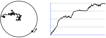
Figure 1: The Brownian carousel and the winding angle $\alpha_{\lambda}$.

The Brownian carousel description gives a simple way to analyze the limiting point process. The hyperbolic angle of the rotating boundary point as measured from $b(t)$ follows the following coupled one-parameter family of stochastic differential equations

$$d\alpha_{\lambda}=\lambda f\,dt+\operatorname{Re}\bigl{(}(e^{-i\alpha_{\lambda}}-1)\,dZ\bigr{)},\qquad\alpha_{\lambda}(0)=0,$$ (5)

driven by a two-dimensional standard Brownian motion and $f$ given in (4). For a single $\lambda$, this reduces to the one-dimensional stochastic differential equation

$$d\alpha_{\lambda}=\lambda f\,dt+2\sin(\alpha_{\lambda}/2)\,dW,\qquad\alpha_{\lambda}(0)=0,$$ (6)

which converges as $t\to\infty$ to an integer multiple $\alpha_{\lambda}(\infty)$ of $2\pi$. In particular, the number of points of the point process $\mathrm{Sine}_{\beta}$ in $[0,\lambda]$ has the same distribution as $\alpha_{\lambda}(\infty)/(2\pi)$ and $p_{\lambda}$ is equal to the probability that $\alpha$ converges to $0$ as $t\to\infty$. See Valkó and Virág (2009) for further details.

In the analysis of equation (6), it helps to remove the space dependence from the diffusion coefficient by a change of variables $X(t)=\log(\tan(\alpha(t)/4))$. The diffusion $X$ satisfies the stochastic differential equation

$$dX=\frac{\lambda}{2}f\cosh X\,dt+\frac{1}{2}\tanh X\,dt+dB,\qquad X(0)=-\infty.$$ (7)

In Valkó and Virág (2009), equations (6) and (7) were used to identify the leading term in the asymptotic expansion of $p_{\lambda}$ in (1). The proof of Theorem 1 requires a more careful analysis of equation (7).

In Lemma 4, we will show that for any initial condition $X(0)=x\in[-\infty,\infty)$ there is a unique solution of the equation given in (7) and the desired gap probability $p_{\lambda}$ may be written in terms of a passage probability for this process. Namely, $p_{\lambda}=p_{\lambda}(-\infty)$ where

$$p_{\lambda}(x) := \mathbf{P}\bigl{(}\mbox{$X(t)$ is finite for all $t>0$ and}$$

$$\quad\mbox{it does not converge to $+\infty$ as $t\to\infty$}\bigr{)}.$$

A time shift of equation (7) only changes the parameter $\lambda$ and the initial condition. This, together with the Markov property of the diffusion $X$, shows that with $T=\frac{4}{\beta}\log\lambda$ we have

$$p_{\lambda} = \mathbf{E}[\mathbf{1}\{\mbox{$X(t)$ is finite for all $0<t\leq T$}\}\cdot p_{1}(X(T))].$$

Our main tool is the Cameron–Martin–Girsanov formula, which allows one to compare the measure on paths given by two diffusions. If we knew the conditional distribution of the diffusion $X$ under the event that it does not blow up, then we could use the Cameron–Martin–Girsanov formula to compute $p_{\lambda}$ explicitly. While we cannot do this, the next best option is to find a new diffusion $Y$ which approximates this conditional distribution. The density (i.e., the Radon–Nikodym derivative) of the path measures given by $Y$ with respect to the measure given by $X$ will be close to the right-hand side of $(\ref{mainform})$. Our strategy for finding $Y$ is described in Section 4. Cameron–Martin–Girsanov techniques have been used to obtain tail asymptotics for the tail asymptotics of the ground state of the random Hill’s equation, see Cambronero, Rider and Ramírez (2006).

In Section 5, we will present a coupling of the transformed processes that enables us to show that the asymptotics is precise up to and including the constant term $\kappa_{\beta}$. The term $\kappa_{\beta}$ is then identified as the expectation of a functional of a certain limiting diffusion.

Open problem

Give an explicit expression for $\kappa_{\beta}$ for general values of $\beta$.

The known values of $\kappa_{\beta}$ are

$$\kappa_{1}=2^{13/24}e^{({3}/{2})\zeta^{\prime}(-1)},\qquad\kappa_{2}=2^{7/12}e^{3\zeta^{\prime}(-1)},\qquad\kappa_{4}=2^{-13/12}e^{({3}/{2})\zeta^{\prime}(-1)},$$

where $\zeta^{\prime}(-1)$ is the coefficient of the linear term in the Laurent series of the Riemann-$\zeta$ function at $-1$.

A natural generalization of Theorem 1 would be to consider the asymptotic probability that there are exactly $k$ eigenvalues in a large interval $[0,\lambda]$. This probability is usually denoted by $E_{\beta}(k;\lambda)$ in the literature. For $\beta=1,2$ and 4 the following large $\lambda$ asymptotics was obtained by Basor, Tracy and Widom (1992):

$$\log E_{\beta}(k;\lambda)=\log E_{\beta}(0;\lambda)+\frac{k\beta}{4}\lambda+\frac{k}{2}\biggl{(}1-\frac{\beta}{2}-\frac{k\beta}{2}\biggr{)}\log\lambda+c_{\beta}+o(1)$$

with explicit constants $c_{\beta}$. [See also Tracy and Widom (1993).] We believe that our methods can be used to extend the previous asymptotics for general values of $\beta$.

The rest of the paper is organized as follows. In the next section, we justify the $p_{\lambda}=p_{\lambda}(-\infty)$ and give some preliminary estimates on the probability $p_{1}(r)$ appearing in (1). Section 3 presents the version of the Cameron–Martin–Girsanov formula that we need. Section 4 describes the strategy for finding $Y$ and Section 5 builds on these sections to complete the proof of the main theorem.

2 Preliminary results

First, we formally verify the connection between the gap probability $p_{\lambda}$ and the diffusion given in (7).

Lemma 4

The diffusion (7) has a unique solution for any initial condition $X(0)=x\in[-\infty,\infty)$ and $p_{\lambda}=p_{\lambda}(-\infty)$.

The change of variables function $\log\tan(\cdot/4)$ is one-to-one on $(0,2\pi)\to\mathbb{R}$. Therefore, even with $-\infty$ initial condition, the diffusion $X$ is well defined and has a unique solution until $\alpha$ reaches $2\pi$, when it blows up. We define $X(t)=\infty$ after this blowup.

Note that for $\lambda>0$ the solution of equation (6) is always monotone increasing at multiples of $2\pi$. See Section 2.2 in Valkó and Virág (2009) for more details. So, if $\alpha(t)\to 0$ as $t\to\infty$ then $0<\alpha(t)<2\pi$ for all $t>0$. This means that $X(t)$ is finite for all $t>0$ and $X(t)$ cannot converge to $\infty$ which proves $p_{\lambda}=p_{\lambda}(-\infty)$.

Next, we prove a preliminary estimate on the blowup probability of the diffusion (7).

Lemma 5

Recall that $p_{1}(x)$ is the probability that the diffusion (7) with $\lambda=1$ and initial condition $X(0)=x$ does not blow up in finite time and does not converge to $+\infty$ as $t\to\infty$. We have

$$0<p_{1}(x)\leq c_{\beta}\exp\biggl{(}-\frac{\beta}{60}e^{x}\biggr{)}.$$

For the upper bound, we first assume that $x>4$. Consider the diffusion

$$dR=\frac{\beta}{16}e^{R-\beta t/4}\,dt+dB,\qquad R(0)=x.$$ (9)

This has the same noise term as $X$. The drift term of $R$ is $\frac{\beta}{16}e^{x-\beta t/4}$, which is dominated by the drift term $\frac{f(t)}{2}\cosh(x)$ of $X$ when $x$ is nonnegative. Thus, while $R$ stays positive, we have $R\leq X$. This means that for every $t>0$ we have

$$p_{1}(x) \leq \mathbf{P}(\mbox{$X$ does not blow up before time }t)$$

$$\leq \mathbf{P}\Bigl{(}\min_{s\in[0,t]}R(s)<0\mbox{ or $R$ does not blow up before time }t\Bigr{)}.$$

The difference $Z=R-B$ satisfies the ODE

$$e^{-Z}\,dZ=\frac{\beta}{16}e^{B-\beta/4t}\,dt,\qquad Z(0)=x.$$ (11)

Integration gives

$$e^{-x}-e^{-Z(t)}=\frac{\beta}{16}\int_{0}^{t}e^{B(s)-\beta/4s}\,ds.$$

This shows that $Z$ is increasing in $t$, in particular $Z(t)\geq x$. So if $\min_{[0,t]}R<0$ then

$$\min_{[0,t]}B<-x.$$

Furthermore, if

$$e^{-x}<\frac{\beta}{16}\int_{0}^{t}e^{B(s)-\beta/4s}\,ds$$ (12)

then $R$ blows up before time $t$. This certainly happens if the minimum of $B$ on the interval $[0,t]$ is not sufficiently small. More precisely, if

$$\frac{e^{-b}}{4}(1-e^{\beta t/4})>e^{-x}$$ (13)

and $\min_{[0,t]}B>-b$ then (12) follows. So if $b<x$, and (13) holds, then the right-hand side of (2) can be bounded above by

$$P\Bigl{(}\min_{[0,t]}B<-b\Bigr{)}=P\bigl{(}|B(t)|>b\bigr{)}\leq\frac{\sqrt{t}}{b}e^{-{b^{2}}/{(2t)}}.$$

We set

$$t=\frac{16}{\beta}e^{2-x},\qquad b=\frac{4e}{\sqrt{30}}<2.$$

As $x>4$, both $b<x$ and (13) are satisfied and we get the upper bound

$$p_{1}(x)\leq\frac{\sqrt{t}}{b}e^{-{b^{2}}/{(2t)}}<c_{\beta}e^{-({\beta}/{60})e^{x}}$$

with $c_{\beta}=\sqrt{{30/\beta}}$. The upper bound for all values of $x$ now follows by changing the constant $c_{\beta}$ appropriately.

For the lower bound note that since the $\operatorname{Sine}_{\beta}$ process is discrete and translation invariant in distribution, there exists $\nu\in(0,1)$ so that $p_{\nu}=p_{\nu}(-\infty)>0$. By the Markov property, we have

$$p_{\nu}=\int_{-\infty}^{\infty}K_{0,1}(-\infty,dx)p_{\nu e^{\beta/4}}(x),$$

where $K_{s,t}(y,dx)$ is the transition kernel of the Markov process $X$ with parameter $\lambda=\nu$. This implies that for some $x_{0}\in\mathbb{R}$ we have

$$p_{\nu e^{\beta/4}}(x_{0})>0.$$

Consider the process $X$ started at $x$ with parameter $\lambda=1$. The Markov property applied at time $t_{0}=1-\frac{4}{\beta}\log\nu$ and the monotonicity of $p_{\lambda}(x)$ in $x$ implies

$$p_{1}(x)\geq P\bigl{(}X(t_{0})<x_{0}\bigr{)}p_{\nu e^{\beta/4}}(x_{0})>0,$$

since $P(X(t)<x)$ is positive for all $x\in\mathbb{R}$ and $t>0$.

3 The Cameron–Martin–Girsanov formula

Our main tool will be the following version of the Cameron–Martin–Girsanov formula. Here, we allow diffusions to blow up to $+\infty$ in finite time, in which case they are required to stay there forever after.

Proposition 6

Consider the following stochastic differential equations:

$$dX = g(t,X)\,dt+dB,\qquad\lim_{t\to 0}X(t)=-\infty,$$ (14)

$$dY = h(t,Y)\,dt+d\tilde{B},\qquad\lim_{t\to 0}Y(t)=-\infty$$ (15)

on the interval $(0,T]$ where $B,\tilde{B}$ are standard Brownian motions. Assume that (14) has a unique solution $X$ in law taking values in $(-\infty,\infty]$.

Let

$$\qquad G_{s}=G_{s}(X)=\int_{0}^{s}\bigl{(}h(t,X)-g(t,X)\bigr{)}\,dX-\frac{1}{2}\int_{0}^{s}\bigl{(}h(t,X)^{2}-g(t,X)^{2}\bigr{)}\,dt$$ (16)

and assume that:

$g^{2}-h^{2}$ and $g-h$ are bounded when $x$ is bounded above. (Then $G_{s}$ is almost surely well defined when $X_{s}$ is finite.)

$G_{s}$ is bounded above by a deterministic constant.

$G_{s}\to-\infty$ when $s\uparrow\tau$ if $X$ hits $+\infty$ at time $\tau$. In this case, we define $G_{s}:=-\infty$ for $s\geq\tau$.

Consider the process $\tilde{Y}$ whose density with respect to the distribution of the process $X$ is given by $e^{G_{T}}$. Then $\tilde{Y}$ satisfies the second SDE (15) and never blows up to $+\infty$ almost surely. Moreover, for any nonnegative function $\varphi$ of the path of $X$ that vanishes when $X$ blows up we have

$$\mathbf{E}\varphi(X)=\mathbf{E}\bigl{[}\varphi(Y)e^{-G_{T}(Y)}\bigr{]}.$$ (17)

Remark 7.

There exist several versions of the Cameron–Martin–Girsanov formula for exploding diffusions [e.g., McKean (2005), Section 3.6]. As we did not find one in the literature which could be directly applied to our case, we sketch the proof below.

Proof of Proposition 6 We follow the standard proof of the Girsanov theorem.

First, we show that $G_{s}$ is well defined for finite $X_{s}$. From condition (A), it follows that the second integral is well defined. The first integral can be written as

$$\int_{0}^{s}(h-g)\,dB+\int_{0}^{s}(h-g)g\,dt$$

which is well defined since $(h-g)$ and $2(h-g)g=(h^{2}-g^{2})-(h-g)^{2}$ when their argument $x$ is bounded above.

Next, we show that $M_{s}=e^{G_{s}}$ is a bounded martingale. This is clear after the hitting time $\tau$ of $X$ of $+\infty$, if such time exists. Before this time, $G_{s}$ is a semimartingale, and so is $M_{s}$. Itô’s formula gives

$$dM=(h-g)M\,dB$$

so that the drift term of $M$ vanishes. So $M$ is a local martingale which is bounded, so it has to be a martingale.

The rest of the proof is standard and is outlined as follows. Set

$$\tilde{B}_{s}=X_{s}-\int_{0}^{s}h\,dt=B_{s}-\int_{0}^{s}(h-g)\,dt.$$

It suffices to show that $\tilde{B}$ is a Brownian motion with respect to the new measure with density $M_{T}$. This follows from Lévy’s criterion [Karatzas and Shreve (1991), Theorem 3.3.16] if $\tilde{B}$ and $\tilde{B}^{2}-s$ are local martingales. Since $M$ is a martingale, it suffices to show that $\tilde{B}M$ and $(\tilde{B}^{2}-s)M$ are local martingales with respect to the old measure, which is just a simple application of Itô’s formula.

The identity (17) is just a version of the change of density formula.

4 Construction of the diffusion $Y$

In this section, we will create a diffusion which approximates the conditional distribution of the diffusion $X$ under the event that it does not blow up. We will construct a drift function $h(t,x)$ for which the diffusion $Y$

$$dY=h(t,Y)\,dt+dB_{t},\qquad Y(0)=-\infty,$$ (18)

is well defined, a.s. finite for $t>0$ and the (formal) Radon–Nikodym derivative $e^{G_{T}}$ with $G_{T}$ defined in (16) is almost equal to the right-hand side of equation (1) with the appropriate $\gamma_{\beta}$.

Lemma 8

For the diffusion (7), $\lambda>1$ and $T=\frac{4}{\beta}\log\lambda$ there exists a function $h(t,x)$ so that conditions (A)–(C) of Proposition 6 hold, and $G_{T}$ has the following form:

$$-G_{T}(X) = -\frac{\beta}{64}\lambda^{2}+\biggl{(}\frac{\beta}{8}-\frac{1}{4}\biggr{)}\lambda+\frac{1}{8}\biggl{(}\beta+\frac{4}{\beta}-6\biggr{)}\log\lambda$$

$${}+\frac{\beta}{8}e^{X(T)}+\biggl{(}2-\frac{\beta}{2}\biggr{)}X(T)^{+}+\omega(X(T))$$

$${}+\int_{0}^{T}\phi\bigl{(}T-t,X(t)\bigr{)}\,dt.$$

Here, the function $\omega$ is bounded and continuous, $\phi$ is continuous and $|\phi(t,x)|\leq\tilde{\phi}(t)$ with $\int^{\infty}_{0}\tilde{\phi}(t)\,dt<\infty$. The functions $\omega$ and $\phi,\tilde{\phi}$ may depend on the parameter $\beta$, but not on $\lambda$.

The function $h$ will have the following form:

$$h(t,x)=-\frac{\lambda}{2}f\sinh(x)+h_{0}(t,x),$$ (20)

where $|h_{0}(t,x)|<c$ if $0\leq t\leq T$. The constant $c$ depends only on $\beta$.

Construction of the function $h$. Given an explicit formula for $h$ it would not be hard to check that ${G_{T}}$ has the desired form. However, we would like to present a way one can find the appropriate drift function. This will provide a better understanding of the form of the resulting $h$.

We will use the definition

$$-G_{s}(X)=\int_{0}^{s}\bigl{(}g(t,X)-h(t,X)\bigr{)}\,dX+\frac{1}{2}\int_{0}^{s}\bigl{(}h^{2}(t,X)-g^{2}(t,X)\bigr{)}\,dt,$$

where

$$g=g_{1}+g_{2},\qquad g_{1}(t,x)=\frac{\lambda}{2}f(t)\cosh x,\qquad g_{2}(t,x)=\frac{1}{2}\tanh x.$$

Our goal is to find the appropriate drift term $h$ in a way that the diffusion $Y$ will approximate the conditional distribution of $X$ given that it does not blow up in the interval $[0,T]$. We will do this term by term, starting with the highest order; toward this end we write $h=h_{1}+h_{2}+h_{3}+h_{4}$. We set

$$h_{1}(t,x)=-\frac{\lambda}{2}f(t)\sinh(x)$$ (21)

as this yields the nice cancelation

$$h_{1}^{2}-g_{1}^{2}=\frac{\lambda^{2}}{4}f(t)^{2}\sinh^{2}(X)-\frac{\lambda^{2}}{4}f(t)^{2}\cosh^{2}(X)=-\frac{\lambda^{2}}{4}f(t)^{2}$$

in the main terms of $h^{2}-g^{2}$. In addition, if the remaining term $h_{2}+h_{3}+h_{4}$ is bounded, then it will be easy to show that conditions (A)–(C) of Proposition 6 are satisfied. This will be done at the end of the proof.

The contribution of the drift terms $h_{1}$ and $g_{1}$ to the stochastic integral part of $-G_{s}$ is given by

$$\frac{\lambda}{2}\int_{0}^{s}f(t)\bigl{(}\cosh(X)-\sinh(X)\bigr{)}\,dX=\frac{\lambda}{2}\int_{0}^{s}e^{X}f(t)\,dX.$$ (22)

Our main tool for evaluating integrals with respect to $dX$ is the following version of Itô’s formula. Let $a,b$ be continuously differentiable functions and let $\tilde{a}$ denote the antiderivative of $a$. Then

$$a(t)b(X)\,dX=d(a(t)\tilde{b}(X))-a^{\prime}(t)\tilde{b}(X)\,dt-\tfrac{1}{2}a(t)b^{\prime}(X)\,dt.$$ (23)

Since $f^{\prime}(t)=-\beta/4f(t)$, and $X(0)=-\infty$, this formula gives

$$\frac{\lambda}{2}\int_{0}^{s}f(t)e^{X}\,dX=\frac{\lambda}{2}f(s)e^{X(s)}+\frac{\lambda}{2}\biggl{(}\frac{\beta}{4}-\frac{1}{2}\biggr{)}\int_{0}^{s}e^{X}f\,dt.$$ (24)

Next, we would like to choose $h_{2}$ in (21) so that the integral term in the right-hand side of (24) simplifies. More precisely, since we expect the diffusion $X$ to be near 0 most of the time, we would like to replace the term $e^{X}$ by $1$. The plan is to use the cross term $\int h_{1}h_{2}\,dt$ in the $\frac{1}{2}\int h^{2}\,dt$ term of $G$ to do this. Namely, we would like to have

$$h_{1}h_{2}=\frac{\lambda}{2}\biggl{(}\frac{\beta}{4}-\frac{1}{2}\biggr{)}(1-e^{x})f.$$ (25)

The solution for (25) is given by

$$h_{2}(t,x)=\biggl{(}\frac{\beta}{4}-\frac{1}{2}\biggr{)}\bigl{(}1+\tanh(x/2)\bigr{)}.$$ (26)

We will choose the next term, $h_{3}$, so that the cross term $\int h_{1}h_{3}\,dt$ in $\frac{1}{2}\int h^{2}\,dt$ cancels the cross term $-\int g_{1}g_{2}$ in $-\frac{1}{2}\int g^{2}\,dt$. This leads to the equation

$$h_{1}h_{3}=g_{1}g_{2}=\frac{\lambda}{2}f(t)\cosh(x)\cdot\frac{1}{2}\tanh(x),$$

which gives

$$h_{3}(t,x)=-\tfrac 12.$$ (27)

Collecting all our previous computations, we get

$$-G_{s} = \frac{\lambda}{2}f(s)e^{X(s)}-\frac{\lambda^{2}}{8}\int_{0}^{s}f^{2}\,dt+\lambda\biggl{(}\frac{\beta}{8}-\frac{1}{4}\biggr{)}\int_{0}^{s}f\,dt$$

$${}+\frac{1}{2}\int_{0}^{s}2h_{1}h_{4}+(h_{2}+h_{3}+h_{4})^{2}-g_{2}^{2}\,dt$$

$${}-\int_{0}^{s}h_{4}\,dX+\int_{0}^{s}(g_{2}-h_{2}-h_{3})\,dX.$$

The integrand $u=g_{2}-h_{2}-h_{3}$ in the last integral of (4) has antiderivative

$$\tilde{u}(x)=\biggl{(}1-\frac{\beta}{4}\biggr{)}x+\biggl{(}1-\frac{\beta}{2}\biggr{)}\log\cosh(x/2)+\frac{1}{2}\log\cosh x.$$ (29)

By Itô’s formula, $\int_{0}^{s}u(X)\,dX-\tilde{u}(X)|_{0}^{s}$ is given by

$$-\frac{1}{2}\int_{0}^{s}u^{\prime}(X)\,dt = -\frac{1}{2}\int_{0}^{s}\biggl{[}\frac{2-\beta}{8}\operatorname{sech}(X/2)^{2}+\frac{1}{2}\operatorname{sech}(X)^{2}\biggr{]}\,dt$$

$$= \frac{\beta-6}{16}s+\int_{0}^{s}\biggl{[}\frac{(2-\beta)}{16}{\tanh(X/2)}^{2}+\frac{1}{4}{{\tanh(X)}^{2}}\biggr{]}\,dt.$$

Note that

$$\lim_{x\to-\infty}\tilde{u}(x)=\frac{\beta-3}{2}\log 2=c_{1}.$$

Substituting this computation for the last integral and expanding $(h_{2}+h_{3}+h_{4})^{2}$, we can rewrite (4) as follows:

$$-G_{s} = -\frac{\lambda^{2}}{8}\int_{0}^{s}f^{2}\,dt+\lambda\biggl{(}\frac{\beta}{8}-\frac{1}{4}\biggr{)}\int_{0}^{s}f\,dt$$

$${}+\biggl{(}\frac{1}{2}\biggl{(}\frac{\beta}{4}-1\biggr{)}^{2}+\frac{\beta-6}{16}\biggr{)}s$$

$${}+\frac{\lambda}{2}f(s)e^{X(s)}+\tilde{u}(X(s))-c_{1}$$

$${}+\frac{1}{2}\int_{0}^{s}\bigl{(}2h_{1}h_{4}+2(h_{2}+h_{3})h_{4}+h_{4}^{2}\bigr{)}\,dt$$

$${}-\int_{0}^{s}h_{4}\,dX+\int_{0}^{s}\eta(X(t))\,dt.$$

The coefficient of $s$ in the first line of (4) comes from the first term on the right-hand side in (4) and the constant term of $(h_{2}+h_{3})^{2}/2$. The function $\eta$ collects the terms from the integrand in (4), the terms $(h_{2}+h_{3})^{2}/2$ with the constant term $(\beta/4-1)^{2}/2$ removed, and $-g_{2}^{2}/2$. More explicitly, we have

$$\eta(x)=\frac{(8-6\beta+{\beta}^{2})}{32}\bigl{(}2\tanh(x/2)+{\tanh(x/2)}^{2}\bigr{)}+\frac{1}{8}(\tanh x)^{2}.$$

The function $\eta(x)$ contributes to an error term that needs to be controlled, but whose precise value does not influence our final result. Now, we are ready to set the value for $h_{4}$: we will choose it in a way that the cross term $\int h_{1}h_{4}\,dt$ in (4) will cancel the integral $\int\eta\,dt$. This gives $h_{4}=-\eta/h_{1}$, that is,

$$h_{4}=\frac{2}{\lambda f(t)}\frac{\eta(x)}{\sinh(x)}.$$ (32)

The function $h_{4}$ is a product of a function of $t$ and a function of $x$. Itô’s formula (23), with the notation $\tilde{h}_{4}(t,x)=\int_{0}^{x}h_{4}(t,y)\,dy$ yields the evaluation of the stochastic integral in (4):

$$-\int_{0}^{s}h_{4}\,dX=-\tilde{h}_{4}(s,X(s))+\frac{\beta}{4}\int_{0}^{s}\tilde{h}_{4}\,dt+\frac{1}{2}\int_{0}^{s}\partial_{x}h_{4}\,dt.$$

Plugging this into (4) and simplifying the deterministic terms in the first line of (4), we arrive at

$$-G_{s} = -\frac{\lambda^{2}}{8}\int_{0}^{s}f^{2}\,dt+\lambda\biggl{(}\frac{\beta}{8}-\frac{1}{4}\biggr{)}\int_{0}^{s}f\,dt+\frac{1}{32}(\beta^{2}+12{\beta}+8)s$$

$${}+\lambda e^{-\beta/4s}\frac{\beta}{8}e^{X(s)}+\tilde{u}(X(s))-c_{1}-\tilde{h}_{4}(s,X(s))$$

$${}+\int_{0}^{s}\biggl{(}2(h_{2}+h_{3})h_{4}+h_{4}^{2}+\frac{\beta}{4}\tilde{h}_{4}+\frac{1}{2}\partial_{x}h_{4}\biggr{)}\,dt.$$

Note that $h_{2}$ and $h_{3}$ do not depend on $t$ and are bounded by an absolute constant. The functions $h_{4},\tilde{h}_{4},\partial_{x}h_{4}$ are all bounded by a constant times $1/(\lambda f(t))=\frac{16}{\beta^{2}}f(T-t)$, which itself is bounded by a constant not depending on $\lambda$ as long as $0\leq t\leq T$. Thus, we can rewrite the integrand in (4) as

$$\int_{0}^{s}\phi\bigl{(}T-t,X(t)\bigr{)}\,dt$$ (34)

with a continuous function $\phi$ which does not depend on $\lambda$ and satisfies $|\phi(t,x)|\leq\tilde{\phi}(t)$ with $\int^{\infty}_{0}\tilde{\phi}(t)\,dt<\infty$. Using (29) and the fact that $\log\cosh x-|x|$ is bounded, the terms in the second line of (4) can be written as

$$\biggl{(}2-\frac{\beta}{2}\biggr{)}X(s)^{+}+\lambda e^{-\beta/4s}\frac{\beta}{8}e^{X(s)}+\omega_{0}(X(s))-\tilde{h}_{4}(T,X(T))$$ (35)

with a bounded and continuous $\omega_{0}$. This concludes the construction of the function $h$. In order to get the expression (8) for $-G_{T}$, we first plug in $s=T$ into (4). Then the first line gives

$$-\frac{\lambda^{2}\beta}{64}(1-\lambda^{-2})+\lambda\biggl{(}\frac{\beta}{8}-\frac{1}{4}\biggr{)}(1-\lambda^{-1})+\frac{1}{4}\biggl{(}\frac{\beta}{2}+\frac{2}{\beta}-3\biggr{)}\log\lambda,$$

and by (35) the second line transforms to

$$\biggl{(}2-\frac{\beta}{2}\biggr{)}X(s)^{+}+\frac{\beta}{8}e^{X(s)}+\omega_{0}(X(T))-\tilde{h}_{4}(T,X(T)).$$

Note that the expression $\tilde{h}_{4}(T,x)$ does not depend on $T$ and is bounded. This proves that $-G_{T}$ is in the desired from (8).

Now, we are ready to check that the proposed choice of $h$ satisfies all the needed conditions (A)–(C).

Condition (A). As $x\to-\infty$, we have

$$g(t,x)=\tfrac 14\lambda fe^{-x}-\tfrac 12+\hat{g}(t,x),\qquad h(t,x)=\tfrac 14\lambda fe^{-x}-\tfrac 12+\hat{h}(t,x),$$

where $|\hat{g}|<ce^{x}$ and $|\hat{h}|<c^{\prime}e^{x}$ with constants that only depend on $\beta$ if $0\leq t\leq T$. From this, it follows that $g-h$ and $g^{2}-h^{2}$ are both bounded if $x$ is bounded from above.

Condition (B). We need that (4) is bounded from below if $0\leq s\leq T$. The integrals in the first line are bounded by a constant depending on $\lambda$ and $\beta$ only. The same is true for the integral in the last line, see (34) and the discussion around it. Thus, we only need to deal with the evaluation terms of the second line. By (35), we just need to show that

$$\biggl{(}2-\frac{\beta}{2}\biggr{)}X(s)^{+}+\lambda e^{-\beta/4s}\frac{\beta}{8}e^{X(s)}$$ (36)

is bounded from below. Since $s\leq T=\frac{4}{\beta}\log{\lambda}$, we get that (36) is bounded from below by

$$\biggl{(}2-\frac{\beta}{2}\biggr{)}X(s)^{+}+\frac{\beta}{8}e^{X(s)}$$

which in turn is bounded from below by a constant depending only on $\beta$.

Condition (C). This follows the same way: one only needs to check the behavior of (36) as $s$ converges to the hitting time of $\infty$. This expression converges to $\infty$ as $X(s)\to\infty$ which means that $G_{s}\to-\infty$.

5 The proof of the main theorem

We are ready to prove Theorem 1.

Proof of Theorem 1 Lemma 4 gives $p_{\lambda}=p_{\lambda}(-\infty)$, where

$$p_{\lambda}(x) = \mathbf{P}\bigl{(}\mbox{$X(t)$ is finite for all $t>0$ and}$$

$$\hskip 13.0pt\hskip 6.0pt\mbox{does not go to $\infty$ as $t\to\infty$}\bigr{)}$$

with $X(0)=x$, as defined in (1). Note that a time shift of equation (7) only changes $\lambda$ and the initial condition. With

$$T=T_{\lambda}=\frac{4}{\beta}\log\lambda$$ (37)

the diffusion $\tau\mapsto X(\tau+T)$ satisfies (7) with $\lambda=1$ and with initial condition $-\infty$ at $\tau=-T$. This suggests that the dependence on $\lambda$ for the probability on the right-hand side of (1) comes mainly from the interval $[0,T]$. Because of this we take conditional expectations in (1) with respect to the $\sigma$-algebra generated by $(X(t),t\in[0,T])$. Using the Markov property of $X$, we obtain

$$p_{\lambda}=\mathbf{E}\bigl{(}\mathbf{1}\{\mbox{$X(t)$ is finite for all $0<t\leq T$}\}\cdot p_{1}(X(T))\bigr{)}.$$ (38)

The first term in the expectation is a function of the path $X(t)$ on the time interval $[0,T]$. Consider a diffusion $Y$ given by the SDE (18) with a drift function $h(t,x)$ given by Lemma 8. With the notation of Lemma 8, we set

$$\qquad\psi(Y)=\biggl{(}2-\frac{\beta}{2}\biggr{)}Y(T)^{+}+\frac{\beta}{8}e^{Y(T)}+\omega(Y(T))+\int_{0}^{T}\phi\bigl{(}T-t,Y(t)\bigr{)}\,dt.$$ (39)

We apply the Girsanov transformation of Proposition 6 together with equation (8) of Lemma 8 to get

$$p_{\lambda}=\lambda^{\gamma_{\beta}}e^{-({\beta}/{64})\lambda^{2}+({\beta}/{8}-1/4)\lambda}\mathbf{E}[p_{1}(Y(T_{\lambda}))\exp\{\psi(Y)\}],$$

where $\gamma_{\beta}=\frac{1}{4}(\frac{\beta}{2}+\frac{2}{\beta}-3).$ In order to prove the theorem, it suffices to show that the limit

$$\lim_{\lambda\to\infty}\mathbf{E}[p_{1}(Y(T_{\lambda}))\exp\{\psi(Y)\}]$$ (40)

exists, and is finite and positive. This limit then equals the constant $\kappa_{\beta}$ of the asymptotics. Recall that in (39) the function $\omega$ is continuous and bounded and $\phi(t,y)$ can be dominated by a function $\tilde{\phi}(y)$ which has a finite integral in $[0,\infty)$.

We will run the process $Y_{\lambda}(t)$ with a shifted time, $\tau=t-T=t-\frac{4}{\beta}\log\lambda$; that is, let

$$\tilde{Y}_{T}(\tau):=Y_{\lambda}(\tau+T).$$

The advantage of this shifted time is that the diffusions $\tilde{Y}_{T}(\tau)$ for different $\lambda$ satisfy the same SDE except they evolve on nested time intervals:

$$d\tilde{Y}_{T}(\tau)=\tilde{h}(\tau,\tilde{Y})\,d\tau+dB,\qquad\tau>-T,\qquad\tilde{Y}_{T}(-T)=-\infty,$$ (41)

where the drift term is given by

$$\tilde{h}(\tau,y)=h(T+\tau,y)=-\frac{\beta}{8}e^{-\beta\tau/4}\sinh(y)+h_{0}(T+\tau,y).$$ (42)

In this new time-frame, we need to show that the limit

$$\lim_{T\to\infty}\mathbf{E}p_{1}(\tilde{Y}_{T}(0))\exp\{\tilde{\psi}(\tilde{Y}_{T})\}$$ (43)

exists, is positive and finite, where

$$\tilde{\psi}(\tilde{Y})=\biggl{(}2-\frac{\beta}{2}\biggr{)}\tilde{Y}(0)^{+}+\frac{\beta}{8}e^{\tilde{Y}(0)}+\omega(\tilde{Y}(0))+\int_{0}^{T}\phi(t,\tilde{Y}(-t))\,dt.$$ (44)

We will drive the diffusions (41) with the same Brownian motion $B(t)$. Then for $T_{1}>T_{2}$ we have $Y_{T_{1}}(\tau)>Y_{T_{2}}(\tau)$ for $\tau\in[T_{2},\infty)$ as this holds for $\tau=-T_{2}$ and the domination is preserved by the evolution.

We also consider a nonnegative-valued diffusion $Z(t)$ given by the SDE

$$dZ=r(Z)\,dt+dB$$

which is reflected at $0$ and whose drift term is equal to

$$r(y)=-\frac{\beta}{16}e^{y}+c_{1}.$$ (45)

We will use the stationary version of $Z$ to dominate the diffusions $\tilde{Y}_{T}$.

By Lemma 8, the term $h_{0}(y,T+\tau)$ in (42) is bounded if $-T\leq\tau\leq 0$. Thus, we can choose the constant $c_{1}$ in (45) so that

$$r(z)\geq\sup_{\{\tau<0,0\leq y\leq z\}}h(\tau,y).$$ (46)

Since $Z$ and $\tilde{Y}$ are driven by the same Brownian motion, if $Z,\tilde{Y}>0$ then $Z-\tilde{Y}$ evolves according to

$$d(Z-\tilde{Y})=[r(Z)-f(t,Y)]\,dt.$$

By (46), this means that if $Z(\tau_{0})\geq\tilde{Y}(\tau_{0})$ for a $\tau_{0}<0$ then this ordering is preserved by the coupling until time 0.

Consider the process $Z$ in its stationary distribution. Then $Z(-T)>\break\tilde{Y}_{T}(-T)=-\infty$ therefore $Z$ dominates $\tilde{Y}_{T}$ on $[-T,0]$. For every fixed $\tau\leq 0$, the random variables $\tilde{Y}_{T}(\tau)$ are increasing in $T$ and bounded by $Z(\tau)$ so

$$\tilde{Y}_{\infty}(\tau)=\lim_{T\to\infty}\tilde{Y}_{T}(\tau)$$

exists and is dominated by $Z(\tau)$. The function $p_{1}(x)$ is continuous so $p_{1}(\tilde{Y}_{T})\to p_{1}(\tilde{Y}_{\infty})$. By (44), we have

$$\tilde{\psi}(\tilde{Y}_{T})=a(\tilde{Y}_{T}(0))+\int_{0}^{T}\phi(t,\tilde{Y}(-t))\,dt,$$

where $a$ is continuous and $\phi(t,y)$ can be dominated by a function $\tilde{\phi}(y)$ which has a finite integral in $[0,\infty)$. Hence, $\tilde{\psi}(\tilde{Y}_{T})\to\tilde{\psi}(\tilde{Y}_{\infty})$ and

$$q_{T}=e^{\tilde{\psi}(\tilde{Y}_{T})}p_{1}(\tilde{Y}_{T})\to q_{\infty}=e^{\tilde{\psi}(\tilde{Y}_{\infty})}p_{1}(\tilde{Y}_{\infty})\qquad\mbox{as }T\to\infty.$$

Using Lemma 5 to estimate $p_{1}(y)$, we get

$$q_{T}\leq c\exp\biggl{\{}(2-\beta/2)\tilde{Y}_{T}(0)^{+}+\frac{\beta}{8}e^{\tilde{Y}_{T}(0)}-\frac{\beta}{60}e^{\tilde{Y}_{T}(0)}\biggr{\}}\leq c^{\prime}\chi(\tilde{Y}_{T}(0)),$$

where $\chi(y)=\exp\{(\frac{\beta}{8}-\frac{\beta}{61})e^{y}\}$. If we prove that $\mathbf{E}\chi(Z(0))<\infty$, then the dominated convergence theorem will imply

$$\mathbf{E}q_{T}\to\mathbf{E}q_{\infty}<\infty,$$ (47)

and the existence of the limiting constant $\kappa_{\beta}$ will be established.

The generator of the reflected diffusion $Z$ is given by

$$\mathcal{L}f=\tfrac 12f^{\prime\prime}+f^{\prime}r$$

for functions $f$ defined on $[0,\infty)$ with $f^{\prime}(0+)=0$ [Revuz and Yor (1999), Chapter VII, Section 3]. Partial integration shows that if $(\log g)^{\prime}=2r$ and $f^{\prime}(0+)=0$ then $\int_{0}^{\infty}\mathcal{L}f(x)g(x)\,dx=0$ which means that

$$g(z)=c\exp(-\beta/8e^{z}+2c_{1}z)$$

gives a stationary density. Since $\int_{0}^{\infty}\chi(z)g(z)\,dz=\mathbf{E}\chi(Z(0))<\infty$, the convergence (47) follows. This shows that

$$\kappa_{\beta}=\mathbf{E}q_{\infty}=\mathbf{E}\bigl{[}e^{\psi(\tilde{Y}_{\infty})}p_{1}(\tilde{Y}_{\infty}(0))\bigr{]}<\infty.$$

The only thing left to prove is that $\kappa_{\beta}=\mathbf{E}q_{\infty}$ is not zero. The definitions of $q$ and $\psi$ yield

$$q_{\infty}\geq cp_{1}(\tilde{Y}_{\infty}(0))e^{(2-\beta/2)Y_{\infty}(0)^{+}}.$$

By Lemma 5, the function $p_{1}(\cdot)$ is positive. Since $\tilde{Y}_{\infty}(0)$ is a.s. finite and we get that $\mathbf{E}q_{\infty}>0$ which completes the proof of Theorem 1.

References

• Basor, Tracy and Widom (1992) {barticle}[mr] \bauthor\bsnmBasor, \bfnmEstelle L.\binitsE. L., \bauthor\bsnmTracy, \bfnmCraig A.\binitsC. A. and \bauthor\bsnmWidom, \bfnmHarold\binitsH. (\byear1992). \btitleAsymptotics of level-spacing distributions for random matrices. \bjournalPhys. Rev. Lett. \bvolume69 \bpages5–8. \biddoi=10.1103/PhysRevLett.69.5, mr=1173848 \endbibitem
• Cambronero, Rider and Ramírez (2006) {barticle}[mr] \bauthor\bsnmCambronero, \bfnmSantiago\binitsS., \bauthor\bsnmRider, \bfnmB.\binitsB. and \bauthor\bsnmRamírez, \bfnmJosé\binitsJ. (\byear2006). \btitleOn the shape of the ground state eigenvalue density of a random Hill’s equation. \bjournalComm. Pure Appl. Math. \bvolume59 \bpages935–976. \biddoi=10.1002/cpa.20104, mr=2222441 \endbibitem
• Chen and Manning (1996) {barticle}[mr] \bauthor\bsnmChen, \bfnmY.\binitsY. and \bauthor\bsnmManning, \bfnmS. M.\binitsS. M. (\byear1996). \btitleSome eigenvalue distribution functions of the Laguerre ensemble. \bjournalJ. Phys. A \bvolume29 \bpages7561–7579. \biddoi=10.1088/0305-4470/29/23/019, mr=1425838 \endbibitem
• Deift et al. (2007) {barticle}[mr] \bauthor\bsnmDeift, \bfnmP.\binitsP., \bauthor\bsnmIts, \bfnmA.\binitsA., \bauthor\bsnmKrasovsky, \bfnmI.\binitsI. and \bauthor\bsnmZhou, \bfnmX.\binitsX. (\byear2007). \btitleThe Widom–Dyson constant for the gap probability in random matrix theory. \bjournalJ. Comput. Appl. Math. \bvolume202 \bpages26–47. \biddoi=10.1016/j.cam.2005.12.040, mr=2301810 \endbibitem
• Deift, Its and Zhou (1997) {barticle}[mr] \bauthor\bsnmDeift, \bfnmPercy A.\binitsP. A., \bauthor\bsnmIts, \bfnmAlexander R.\binitsA. R. and \bauthor\bsnmZhou, \bfnmXin\binitsX. (\byear1997). \btitleA Riemann–Hilbert approach to asymptotic problems arising in the theory of random matrix models, and also in the theory of integrable statistical mechanics. \bjournalAnn. of Math. (2) \bvolume146 \bpages149–235. \biddoi=10.2307/2951834, mr=1469319 \endbibitem
• des Cloizeaux and Mehta (1973) {barticle}[mr] \bauthor\bparticledes \bsnmCloizeaux, \bfnmJ.\binitsJ. and \bauthor\bsnmMehta, \bfnmM. L.\binitsM. L. (\byear1973). \btitleAsymptotic behavior of spacing distributions for the eigenvalues of random matrices. \bjournalJ. Math. Phys. \bvolume14 \bpages1648–1650. \bidmr=0328158 \endbibitem
• Dyson (1962) {barticle}[mr] \bauthor\bsnmDyson, \bfnmFreeman J.\binitsF. J. (\byear1962). \btitleStatistical theory of the energy levels of complex systems. II. \bjournalJ. Math. Phys. \bvolume3 \bpages157–165. \bidmr=0143557 \endbibitem
• Ehrhardt (2006) {barticle}[mr] \bauthor\bsnmEhrhardt, \bfnmTorsten\binitsT. (\byear2006). \btitleDyson’s constant in the asymptotics of the Fredholm determinant of the sine kernel. \bjournalComm. Math. Phys. \bvolume262 \bpages317–341. \biddoi=10.1007/s00220-005-1493-4, mr=2200263 \endbibitem
• Karatzas and Shreve (1991) {bbook}[mr] \bauthor\bsnmKaratzas, \bfnmIoannis\binitsI. and \bauthor\bsnmShreve, \bfnmSteven E.\binitsS. E. (\byear1991). \btitleBrownian Motion and Stochastic Calculus, \bedition2nd ed. \bseriesGraduate Texts in Mathematics \bvolume113. \bpublisherSpringer, \baddressNew York. \bidmr=1121940 \endbibitem
• Krasovsky (2004) {barticle}[mr] \bauthor\bsnmKrasovsky, \bfnmI. V.\binitsI. V. (\byear2004). \btitleGap probability in the spectrum of random matrices and asymptotics of polynomials orthogonal on an arc of the unit circle. \bjournalInt. Math. Res. Not. \bvolume25 \bpages1249–1272. \biddoi=10.1155/S1073792804140221, mr=2047176 \endbibitem
• McKean (2005) {bbook}[mr] \bauthor\bsnmMcKean, \bfnmHenry P.\binitsH. P. (\byear2005). \btitleStochastic Integrals. \bpublisherAMS Chelsea Publishing, Providence, RI. \bidmr=2169626 \endbibitem
• Ramírez, Rider and Virág (2007) {bmisc}[auto:SpringerTagBib—2009-01-14—16:51:27] \bauthor\bsnmRamírez, \bfnmJ.\binitsJ., \bauthor\bsnmRider, \bfnmB.\binitsB. and \bauthor\bsnmVirág, \bfnmB.\binitsB. (\byear2007). \bhowpublishedBeta ensembles, stochastic Airy spectrum, and a diffusion. Available at math/0607331. \endbibitem
• Revuz and Yor (1999) {bbook}[mr] \bauthor\bsnmRevuz, \bfnmDaniel\binitsD. and \bauthor\bsnmYor, \bfnmMarc\binitsM. (\byear1999). \btitleContinuous Martingales and Brownian Motion, \bedition3rd ed. \bseriesGrundlehren der Mathematischen Wissenschaften [Fundamental Principles of Mathematical Sciences] \bvolume293. \bpublisherSpringer, \baddressBerlin. \bidmr=1725357 \endbibitem
• Tracy and Widom (1993) {bincollection}[mr] \bauthor\bsnmTracy, \bfnmCraig A.\binitsC. A. and \bauthor\bsnmWidom, \bfnmHarold\binitsH. (\byear1993). \btitleIntroduction to random matrices. In \bbooktitleGeometric and Quantum Aspects of Integrable Systems (Scheveningen, 1992). \bseriesLecture Notes in Physics \bvolume424 \bpages103–130. \bpublisherSpringer, \baddressBerlin. \bidmr=1253763 \endbibitem
• Valkó and Virág (2009) {barticle}[mr] \bauthor\bsnmValkó, \bfnmBenedek\binitsB. and \bauthor\bsnmVirág, \bfnmBálint\binitsB. (\byear2009). \btitleContinuum limits of random matrices and the Brownian carousel. \bjournalInvent. Math. \bvolume177 \bpages463–508. \biddoi=10.1007/s00222-009-0180-z, mr=2534097 \endbibitem
• Widom (1994) {barticle}[mr] \bauthor\bsnmWidom, \bfnmHarold\binitsH. (\byear1994). \btitleThe asymptotics of a continuous analogue of orthogonal polynomials. \bjournalJ. Approx. Theory \bvolume77 \bpages51–64. \biddoi=10.1006/jath.1994.1033, mr=1273699 \endbibitem
• Wigner (1951) {barticle}[mr] \bauthor\bsnmWigner, \bfnmEugene P.\binitsE. P. (\byear1951). \btitleOn a class of analytic functions from the quantum theory of collisions. \bjournalAnn. of Math. (2) \bvolume53 \bpages36–67. \bidmr=0039059 \endbibitem
• Wigner (1952) {barticle}[mr] \bauthor\bsnmWigner, \bfnmE. P.\binitsE. P. (\byear1952). \btitleOn the connection between the distribution of poles and residues for an $R$ function and its invariant derivative. \bjournalAnn. of Math. (2) \bvolume55 \bpages7–18. \bidmr=0046433 \endbibitem
• Wigner (1957) {bmisc}[auto:SpringerTagBib—2009-01-14—16:51:27] \bauthor\bsnmWigner, \bfnmE. P.\binitsE. P. \bhowpublished(1957). Gatlinburg Conference on Neutron Physics. Report 2309:59, Oak Ridge National Laboratory, Oak Ridge, TN. \endbibitem