Multi-Scale CLEAN: A comparison of its performance against classical CLEAN on galaxies using THINGS

Abstract

A practical evaluation of the Multi-Scale clean algorithm is presented. The data used in the comparisons are taken from The H i Nearby Galaxy Survey (THINGS). The implementation of Multi-Scale clean in the CASA software package is used, although comparisons are made against the very similar Multi-Resolution clean algorithm implemented in AIPS. Both are compared against the classical clean algorithm (as implemented in AIPS). The results of this comparison show that several of the well-known characteristics and issues of using classical clean are significantly lessened (or eliminated completely) when using the Multi-Scale clean algorithm. Importantly, Multi-Scale clean reduces significantly the effects of the clean ‘bowl’ caused by missing short-spacings, and the ‘pedestal’ of low-level un-cleaned flux (which affects flux scales and resolution). Multi-Scale clean can clean down to the noise level without the divergence suffered by classical clean. We discuss practical applications of the added contrast provided by Multi-Scale clean using two selected astronomical examples: H i holes in the interstellar medium and anomalous gas structures outside the main galactic disk.

1. Introduction

The art of astronomical observations lies in reconstructing the highest fidelity representation of the sky, given the inherent limitations of the data, which are always to some degree affected by atmosphere, instrument, technique or telescope. Some kind of processing always needs to be applied to minimize these issues and produce the most accurate representation of the astronomical source of interest. This processing is particularly important for observations obtained with radio synthesis telescopes, e.g., observations of the $21$cm line of atomic hydrogen. Even though, in this domain, instrumental artifacts are generally small and the atmosphere is well-behaved, the noise and instrumental response (or Point Spread Function, PSF) are still a major problem in generating a true representation of a source. For radio interferometers, the full width at half maximum (FWHM) of the PSF to first order depends on the length of the longest baseline. The precise shape of the PSF and the surface brightness sensitivity depend, however, on the configuration of the array and its filling factor. The incompletely sampled size-scale distribution inherent to an unfilled aperture instrument leads to a complicated PSF and consequently to an image with significant artifacts (we refer the reader to Thompson et al. 2001 for more details).

Deconvolution is the technique of choice for attempting to remove these artifacts. It does so by interpolating and extrapolating the incompletely sampled uv plane, thus attempting to correct for the effects of the complex PSF. Other factors that influence the observations, such as noise and atmospheric effects, cannot be corrected by deconvolution. Deconvolution can be thought of as a simple equation: $(F+G)*H\leavevmode\nobreak\ =\leavevmode\nobreak\ I$, where $(F+G)*H$ indicates the convolution of $F$ plus $G$ with $H$. $F$ is the true image, $G$ is the noise, $H$ is the PSF and $I$ represents the raw measurements or observations. Deconvolution is the process of solving for $F$, given $G$, $H$ and $I$. A measure for the performance of any deconvolution algorithm thus lies in its effectiveness of reducing the effect of a complex PSF ($H$) on the image ($F$). Data that are not (or cannot be) recorded at the telescope, due to, for example, incomplete sampling of the uv-plane are not recovered through deconvolution, but have to be interpolated. This interpolation is at the heart of some of the complications with deconvolution described in this paper.

The ‘de-facto’ standard of deconvolution algorithms for radio astronomy is the clean algorithm (Högbom 1974). This classical clean is an iterative procedure. It assumes that the sky is only sparsely filled with a limited number of point sources superimposed on an otherwise empty background. It finds the location and strength of all these sources, and uses them to reconstruct a representation of the true image using an ideal PSF. Over the years several variants (e.g., Schwab 1984; Clark 1980) have been proposed to overcome various limitations and nuances that are intrinsic to clean (see also Schwarz 1978; Brinks & Shane 1984). However, there still remains a basic assumption that the sky is composed of point sources, which is adequate if the source being observed has limited extent. Extended structure is modeled by clean as a large number of point sources and the iterative procedure becomes a time-consuming process involving a constantly increasing number of point sources. To partly compensate for this problem, clean can be restricted to only work in regions where the source of interest is known to exist, through the use of clean ‘windows’. Such windows require prior knowledge of the source structure and extent, but are flexible and multiple windows can be used to bound a complicated source.

An obvious enhancement to clean would be to make it more efficient at modeling extended structures. Many such ‘scale-sensitive’ algorithms have been proposed. These methods generally assume that the sky is not composed of only point-sources as clean does, but of sources of many different sizes and scales. One of the first such methods, multi-resolution clean, tackles the problem by smoothing and decimating the dirty image and PSF to emphasize the extended emission. The image resulting from cleaning this dirty image is then used as an initial model for cleaning the next higher resolution image, etc. (Wakker & Schwarz 1988). Wavelet clean uses the wavelet transform in the clean process but basically operates in a similar manner to multi-resolution clean (Starck et al. 1994). The more recently developed Adaptive Scale Pixel clean uses scale sizes that can ‘adapt’ their size during processing (Bhatnagar & Cornwell 2004). There is a wealth of literature explaining the inner workings of multi-resolution clean and the other algorithms mentioned above in detail (see Bhatnagar & Cornwell 2003; Starck et al. 2002, in addition to the references above), including a considerable amount of modeling as well as some practical tests.

Multi-scale clean (hereafter referred to as msclean) is a straight-forward extension of the classical clean algorithm for handling extended sources (Cornwell 2008). Just like the multi-resolution clean defined by Wakker & Schwarz (1988), it works by assuming the sky is composed of emission at different spatial scales. However, whilst the Wakker & Schwarz multi-resolution clean works on each scale sequentially, msclean works simultaneously on all scales that are being considered. This prevents potential errors made at a previous larger scale from being ‘frozen in’ and requiring many iterations at smaller scales to correct. msclean has been implemented in both CASA (formerly AIPS++) and classical AIPS (as part of the multi-resolution options of the IMAGR task). In this paper, we compare the operation of msclean against classical clean both with and without the use of clean windows, using some real-world data and astronomical problems derived from high quality HI data obtained through the THINGS project. We refer to Cornwell (2008) for a more technical description of msclean, as well as a description of tests involving artificial data.

THINGS, The H i Nearby Galaxy Survey, consists of a sample of 34 nearby galaxies observed with the NRAO Very Large Array (VLA) B,C and D arrays (Walter et al. 2008). The high resolution ($\sim 6\arcsec$, $\sim 5$ km s^-1) achieved with THINGS pushes the VLA to the limits of its current performance for observations of a significant sample of galaxies. The THINGS observations, being combined multi-array data with a large range of spatial scales therefore present one of the most challenging data-sets with which to compare the efficiency of deconvolution algorithms. We emphasize that classical clean works very well on the THINGS data sets, and that with a full knowledge of its intricacies excellent results can be achieved. However, clean is not perfect, and our goal in this paper is to describe some practical applications of the msclean algorithm. msclean seems to have fewer limitations than clean does when it comes to handling data of extended sources. It is promising enough that it might point the way to an efficient exploration of the high-quality data, similar to the THINGS data set, that will be routinely produced by the next-generation radio and millimeter facilities such as ALMA, EVLA, LOFAR and SKA

This paper begins with a brief description of the clean and msclean algorithms in Section 2. In addition to summarizing the procedure each algorithm uses in Sections 2.1 and 2.2, the paper discusses the limitations of the clean algorithm and the advantages that msclean provides (Section 2.3). In Section 3, a detailed comparison of the performance of clean and msclean on a sample of three galaxies from THINGS is presented. Section 4 then presents a practical comparison between msclean as implemented in CASA, the version implemented in AIPS and classical clean as well as windowed-clean. Having compared msclean to a number of related algorithms, the paper then takes this comparison a step further by describing some astrophysical applications of msclean, namely the detection of structures within the H i disks of galaxies but also the detection of anomalous gas structures outside the disk, in Section 5. The paper ends with a short summary of the key results of the tests and comparisons performed (Section 6).

2. Deconvolution with CLEAN and MSCLEAN

Excellent detailed descriptions of the clean algorithm can be found in Högbom (1974), Schwarz (1978) and Cornwell et al. (1999). For msclean, Cornwell (2008) contains a detailed description of this algorithm. For completeness, and to introduce some nomenclature, we briefly describe the classical clean  as well as the msclean procedure here.

Deconvolution algorithms attempt to create a model of the true ‘sky brightness distribution’ (the object) from the ‘dirty map’ (the observed image) using the ‘dirty beam’ (the observed PSF). This model is called the ‘clean map’ (or ‘restored map’) and is created using the ‘clean beam’, which represents an ideal PSF. It is typically a Gaussian function of the same FWHM as the central component of the dirty beam (Schwarz 1978).

2.1. The CLEAN Procedure

The clean algorithm is an iterative procedure operating on the dirty map. clean can be described as follows:

1. Find the location of the maximum absolute brightness point source in the ‘dirty map’ and optionally within a user-defined window in the image.

2. Multiply the strength of this point source by a gain factor (usually $10$%) to generate a ‘clean component’ at this location.

3. Convolve the clean component with the ‘dirty beam’, and subtract this from the dirty map, recording the position and strength of the clean component subtracted.

4. Repeat the above three steps on the dirty map, until all emission is found, or a certain flux threshold is reached, or a number of iterations has been achieved.

After the procedure has stopped by meeting one of the conditions in Step 4, the result is a list of clean components, and a residual image with all flux cleaned away to the specified conditions. The final image (the clean map or restored image) is created by adding all of the clean components convolved with the clean beam onto the residual map. Adding the residual image left after the iterative subtraction procedure is in principle optional, but is usually always done in order to retain information on the noise and any remaining residual flux (Schwarz 1978). We defer to Section 2.3 a discussion on the potential problem of combining cleaned and uncleaned data.

2.2. The Multi-Scale CLEAN Procedure

Multi-Scale clean (in both its CASA and AIPS implementations) is a modification of the classical clean algorithm. Instead of representing the sky as empty and containing a limited number of point sources as is done by clean, msclean presumes that sources in the sky are actually extended structures of different scales (which can include point sources).

An important constraint is that the function used to define the shape of the scales has a finite extent, so that, for example, a clean window can be applied. As such, a Gaussian function is not a good choice, unless some kind of truncating function is applied. Generally, a paraboloid with an appropriate tapering function is chosen, which becomes a delta-function in the limit of zero scale-size (Cornwell 2008). By pre-computing the convolution of the dirty beam with each scale size, one can proceed with a parallel clean-like procedure on a set of images generated for each of the scales. It is important to include a scale-size zero delta-function which enables proper fitting of point sources. The process is then as follows:

1. Convolve the dirty map with each scale size to create a set of convolved images.

2. Find the global peak among these images, i.e., the scale that contains the maximum total flux and record the position, flux and scale size for the image in which this occurs.

3. Subtract the pre-computed scale (of the same size in which the peak was found) convolved by the dirty beam, multiplied by some gain factor, from all the images made in the first step.

4. Store the subtracted component and the scale size in a table.

5. Repeat the above steps on the current convolved images until all emission has been removed, a flux threshold is reached or an iteration limit has passed.

In other words, where clean operates on a single residual image, msclean keeps a set of residual images, one image per scale size defined. The peak subtraction is performed on all of these images, but only the one subtracted component and its scale size are stored in the clean component table. The restoration is then an addition of the appropriately scaled, positioned and convolved components subtracted at each iteration on top of the final residual image. We refer to Cornwell (2008) for a technical description of the algorithm.

2.3. The Limitations of CLEAN and MSCLEAN’s Advantages

For purely practical reasons, any implementation of clean will have an iteration limit built in (e.g., Cornwell et al. 1999). The design of the algorithm is to iteratively find and remove the strongest point sources; the number of iterations is therefore one of the factors that defines how deep clean will go in terms of the flux level. Eventually, noise peaks will start to be cleaned away as well, as the algorithm cannot distinguish them from faint real signals. The number of components will therefore start to increase dramatically. This can easily spiral out of control as clean approaches the noise limit and leads to a diverging total flux (Cornwell et al. 1999). All of this illustrates the necessity of imposing a hard limit on the number of iterations, either directly or through a flux threshold.

However, despite its usefulness in placing a practical constraint on clean, the iteration limit is not without its disadvantages. It is a compromise between cleaning as deeply as possible and avoiding most of the noise. As mentioned in the introduction, this is a particularly important point for extended sources (such as the THINGS galaxies), which clean will attempt to model with a large number of point sources. In contrast, practical results show that msclean removes large-scale structure before finer details (Cornwell 2008, and see Section 3.2). This provides a useful advantage over clean in most cases: the prior removal of underlying extended emission will reduce the strength of small-scale emission peaks that will remain. This means that when msclean begins to remove the small-scale structure, it will require fewer iterations to do so. The lack of this scale-size advantage in classical clean means it is required to slowly cut down sources. msclean, with its convergence from large to small scales, does not spend its final cycles slowly removing a large amount of extended emission in small increments.

Classical clean must also use low loop gains (typically $10$% or less) to improve the reconstruction of extended emission. Using a high loop gain would be more efficient, especially for extended sources, but can easily lead to instabilities (Cornwell et al. 1999). Furthermore the gain is one parameter of clean that has a large effect on the final clean solution (Schwarz 1978; Tan 1986). msclean is much less dependent on the gain and is able to use much higher values (Cornwell 2008). This means that each msclean scale has the ability to remove a much larger portion of the flux in each individual iteration, again reducing the overall number of iterations required compared to clean.

The problem whereby clean poorly models extended emission is further compounded by the interpolation for the missing spacing information. Generally, in interferometric observations, the extremely short or zero spacings, which measure the largest structure on the sky, are missing. In other words, the innermost part of the uv-plane is not (well) sampled. In these cases the total flux of an extended source (i.e., containing structures at scales larger than sampled by the shortest baseline) cannot be recovered. Together with the strong side-lobes present in the dirty beam and the pedestal of uncleaned flux, this leads to a clean ‘bowl’: the source sits in a region with a negative background. This clean bowl will cause skewed noise and flux estimates. The higher efficiency of msclean in removing extended structures means it can approach the noise limit more easily than clean, with the result that the presence of the clean bowl is also greatly reduced yielding a noise-like residual background.

A subtle, but important limitation of clean lies in the reconstruction of the clean or restored image from the final residual image and the clean components. The restored image is an addition of two separate flux scales, a residual map with the units Jy per dirty beam and a clean component map with units Jy per clean beam. As the extent of the dirty beam is always larger than that of the best-fitting clean beam, using the clean beam to determine the flux of the residuals will always lead to an overestimate of this flux. As such a correction factor needs to be applied to determine the flux in regions with signal (Jörsäter & van Moorsel 1995). This is described in Walter et al. (2008) for the THINGS galaxies. This scaling of the residuals, and therefore the noise, yields correct fluxes in areas with signal, however the noise properties are no longer representative. Residual-scaled cubes should thus be only used to measure fluxes in areas with significant signal. Any other applications which critically depend on noise properties (such as profile fitting) should use the unscaled cubes (see Walter et al. 2008, for a detailed discussion).

In order to illustrate the limitations of clean and potential advantages that msclean could provide, the remainder of this paper is devoted to a practical comparison between clean and msclean (Section 3). We also compare the implementation of msclean in the CASA and AIPS software packages to classical clean with the use of clean windows (Section 4). We use a small sample of galaxies from THINGS to compare the results.

3. A Detailed CLEAN and MSCLEAN Comparison

3.1. Data Processing

We chose three galaxies from the THINGS survey to use for our comparison of msclean and clean. These galaxies are NGC 2403 (catalog ), Holmberg II (catalog ) and IC 2574 (catalog ) and they cover a range of H i masses and morphologies (Walter et al. 2008). Each galaxy was observed with the VLA in B, C and D configurations. This study uses the calibrated and combined uv data-set from all arrays for each galaxy. More details on the observations and generation of the uv data-sets can be found in Walter et al. (2008). The msclean implementation in the CASA software package and the clean implementation in the AIPS software package (based on the Clark clean, see Clark 1980) was used on the uv data-set for this comparison. For each galaxy, two data cubes were generated with two different weightings; a ‘natural’ weighting and a ‘robust’ weighting with a robustness parameter of $0.5$ (Briggs 1995). These weightings were the same as used in the creation of the original THINGS data cubes.

The data cubes were created with the same spatial and velocity pixel sizes as the original THINGS cubes (for details see Walter et al. 2008). The cubes were then ‘msclean-ed’ down to $2.5\sigma$ which was also the flux threshold used in THINGS. As mentioned in Section 2.3, msclean can usually use much higher gain factors than classical clean. In this study, the msclean gain factor was set at $0.7$ for all three galaxies (see Cornwell 2008, for a discussion of the msclean loop gain). No clean windows were used. A maximum number of msclean iterations of $1200$ (NGC 2403), $700$ (Holmberg II) and $1000$ (IC 2574) were chosen for each galaxy per channel. In all cases the flux limit was reached well before the iteration limit. Unless mentioned otherwise below, the cubes were also corrected for primary beam attenuation using the linmos task of the MIRIAD software package. Residual cubes were also created for the clean and msclean data.

3.2. MSCLEAN Scale Choice

As discussed briefly in Section 2.2, CASA (and AIPS++) use paraboloids for the shape of the scale components. Extensive experimentation shows that the results did not depend significantly on the number of scales chosen nor their distribution. The most important choice is that of the largest size in the distribution. We found that optimum results were obtained when this was chosen to correspond roughly to the size of the largest coherent structures visible in individual channel maps. This choice does not have to be exact. We chose a total of six scales distributed where each scale is three times larger than the preceding scale. Again, this choice was not critical, but we found that this distribution was more efficient (in terms of number of iterations required) than a linear distribution. The largest scale for each galaxy was $130\arcsec$ (NGC 2403), $270\arcsec$ (Holmberg II) and $160\arcsec$ (IC 2574).

For comparison, Figure 1 shows how the range of scales chosen and structure size for a single channel map are related in the galaxy NGC 2403. It can be seen that for the largest scale size, the largest coherent structure visible in the channel map fits within its diameter. Choosing an even larger scale would have no effect, as the largest structure is already optimally contained within the scale distribution shown, and msclean would simply not choose these even larger scales. Choosing a smaller, largest scale would simply increase the number of iterations.

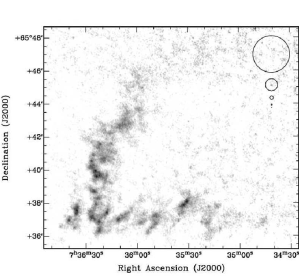
Figure 1.— The relationship between the msclean scale sizes and structure in a single velocity channel of NGC 2403. The upper right corner shows the msclean scale sizes used in processing this galaxy, from largest to smallest down the figure. All scales excluding the smallest scale (a delta peak) are shown. The diameters of the scales are $130\arcsec$, $44\arcsec$, $13\arcsec$, $4\arcsec$ and $1.3\arcsec$. The largest scale size ($130\arcsec$) roughly corresponds to the largest coherent structure visible in the channel map. This relation was used as the basis for choosing the msclean scales to be used for each galaxy, as discussed in Sec. 3.2.

Figure 2 shows the choice of scales the algorithm made with iteration number for a single velocity channel of Holmberg II. In other words, the figure shows the msclean scale component used as the algorithm progressed to lower flux levels. A similar trend is observed across all channels of all three galaxies. It shows that msclean indeed removes emission at larger scales before smaller scales (as explained in Section 2.3).

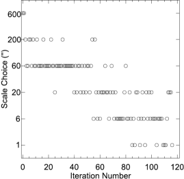
Figure 2.— The choice of scale size with iteration number for a single velocity channel from Holmberg II in msclean . The x-axis shows the iteration number and the y-axis shows the scales (in arc-seconds). As shown, msclean uses the largest scales first, which corresponds to extended emission, before switching to smaller scales and cleaning finer structure.

3.3. Beams

In Table 1 we compare the sizes of the restoring beams of the AIPS clean and the CASA/AIPS++ msclean. These are both determined by fitting a Gaussian function to the central component of the respective dirty beams. As their dirty beams are identical, the small differences seen in Table 1 are due to the different fitting procedures for a Gaussian function used in the restore processes of both software packages.

Table 1FWHM Beam Size Comparison for clean and msclean data.

Source	Weighting	Beam Size ($\arcsec$)
		NGC 2403	Holmberg II	IC 2574
clean	Natural	$8.8\times 7.7$	$13.7\times 12.6$	$12.8\times 11.9$
	Robust	$6.0\times 5.2$	$7.0\times 6.1$	$5.9\times 5.5$
msclean	Natural	$8.0\times 7.1$	$11.4\times 10.9$	$10.8\times 10.3$
	Robust	$5.7\times 4.9$	$6.6\times 5.8$	$6.3\times 5.9$

In Figure 3 profiles of the restoring beams for both weightings and both data-sets are plotted against the respective dirty beam. It should be noted that natural weighting results in a beam that cannot be well approximated by a Gaussian function as shown in these figures. The natural dirty beam has extended ‘wings’, while for a robust dirty beam these wings are much less pronounced and a Gaussian function is a much better fit.

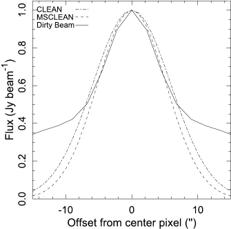
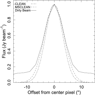
Figure 3.— Profiles of the dirty beam (solid lines) and restoring or clean beams for both clean (dot-dash lines) and msclean (dashed lines) for the natural weighted (left) and robust weighted (with a robustness parameter of $0.5$, right) data of the galaxy IC 2574. The dirty beam for the natural weighted data on the left shows the significant wings which make it difficult to fit a Gaussian function to it. Nevertheless, the restoring beams of clean and msclean are very similar for this weighting. On the other hand, The restoring beams for the robust weighted data are very similar and provide a good fit to the dirty beam, which is approximated well by a Gaussian function.

Natural weighting is more sensitive to diffuse, extended emission. This is where clean is at its weakest. The wings observed in the natural beam (Figure 3, left image) result in a large difference of the beam integral between the natural dirty and restoring beams. Robust weighting (Figure 3, right image) on the other hand is a much better fit to the actual dirty beam. So residual scaling for robust weighting is less important as there is less emphasis on extended structure. Therefore msclean and clean results are much more similar for robust weighting in the case of the THINGS data. In the remainder of this comparison, the paper focuses on the analysis based on the natural weighted data.

3.4. Channel Maps

A comparison of selected single channel maps for both the clean and msclean natural-weighted cubes, including the respective residual channel maps, are shown in Figures 4 to 6. The channel maps shown in these figures are from the non-residual scaled, unmasked THINGS cubes before correcting for primary-beam attenuation.

The clean bowl is most noticeable in the NGC 2403 channel map (Figure 4), obscuring the noise in the inner region of the image. The clean residuals also show a significant pedestal. This contributes to the difference in contrast between regions of low and high flux across the clean and msclean data. For example, the extent of the high-contrast regions (black) are much larger in the channels from the clean data. This pedestal also covers up the ‘holes’ in the flux in the clean images, where in the msclean images one can see right down to the noise levels in these regions, as most readily seen in the channel map for Holmberg II (Figure 5).

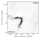
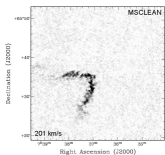
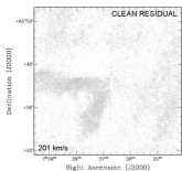
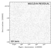
Figure 4.— Comparison of a single channel map of NGC 2403 for the clean (left) and msclean (right) data (top panels). Also shown is the respective residual channel map for the clean (left) and msclean (right) data (bottom panels), which is the clean or msclean channel without adding in the convolved clean components. The channel maps were extracted from the natural-weighted, unmasked cubes. No primary beam correction has been applied. The clean channel maps have not been residual corrected. The gray-scale levels run from $0$ to $4$ mJy beam^-1.

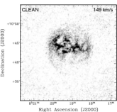
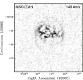
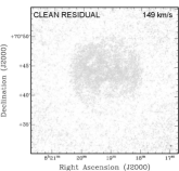
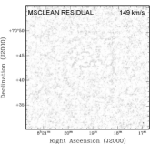
Figure 5.— Comparison of a single channel map of Holmberg II for the clean (left) and msclean (right) data (top panels). Also shown is the respective residual channel map for the clean (left) and msclean (right) data (bottom panels). The channel maps were extracted from the natural-weighted, unmasked cubes. No primary beam correction has been applied. The clean channel maps have not been residual corrected. The gray-scale levels run from $0$ to $10$ mJy beam^-1.

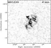
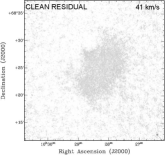
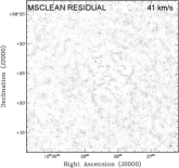
Figure 6.— Comparison of a single channel map of IC 2574 for the clean (left) and msclean (right) data (top panels). Also shown is the respective residual channel map for the clean (left) and msclean (right) data (bottom panels). The channel maps were extracted from the natural-weighted, unmasked cubes. No primary beam correction has been applied. The clean channel maps have not been residual corrected.The gray-scale levels run from $0$ to $6$ mJy beam^-1.

3.5. Integrated H I Maps

Integrated H i maps, as well as integrated residual maps for each galaxy are shown in Figures 7, 8 and 9 for the msclean and clean natural-weighted, primary-beam corrected (and for clean, residual-scaled) data. The cubes were masked with the same masks applied to the clean data (see Walter et al. 2008, for a description of the masking process). The residual integrated maps were generated from residual cubes, i.e., cubes that were cleaned but did not have the clean components added to them. These integrated maps have not been corrected for primary-beam attenuation and for the clean data, no residual scaling has been applied.

The masking applied to the integrated maps hides the signature of the clean bowl seen in the channel maps of the clean data in Figures 4 to 6. The residual integrated clean maps in Figures 7 to 9 do show a significant pedestal of uncleaned flux, while the msclean residual maps have no such feature. There is trace source emission in the msclean residual integrated maps, but generally the residuals are much more ‘noise-like’. Despite being on the same flux scale, there is a definite visual difference between the clean and msclean data, most clearly seen where there is significant source flux (the darker regions) in Holmberg II and IC 2574. Conversely the low-level extended structure is more clearly seen in the msclean integrated maps and extends out to the mask boundary. The peak flux for compact features is therefore higher in the clean integrated images, while the total flux of the underlying, extended structure is greater in msclean.

To compare the flux scales between the data-sets, contour lines of column density $1\cdot 10^{21}$ and $2\cdot 10^{21}$ cm^-2 have been plotted on the (residual scaled) clean and msclean data for each galaxy, shown in Figures 10, 11 and 12. Again, this data has been masked and corrected for primary-beam attenuation. The location of the contours match closely across the clean and msclean data, but they appear much smoother in the clean data. The contours in the msclean images for each galaxy appears to trace a much finer structure boundary. This is likely due to the pedestal of leftover flux in classical clean. The pedestal still has the dirty beam as its PSF, the more extended wings of this beam will wash out structure more severely than a Gaussian beam, and the low-level, small-scale structure will be lost in the image. For low-level column densities the clean resolution is thus worse than one would expect on the basis of the clean beam size, as we will show later. In msclean there is no pedestal, and all fine-scale structure is imaged at the full resolution of the clean beam, enhancing the detailed structures in the disk.

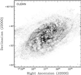
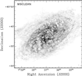
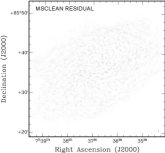
Figure 7.— clean (left) and msclean (right) integrated H i maps (top row) for NGC 2403. The maps were generated from the natural-weighted, masked, primary-beam corrected and for clean, residual flux corrected cubes. The equivalent residual integrated H i maps are also shown (bottom row), generated as described in Sec. 3.5. No primary-beam corrections and for clean, no residual flux corrections have been applied to these images. The gray-scale levels run from $0$ to $200$ mJy beam^-1 km s^-1. Beams are marked in bottom right corner of images.

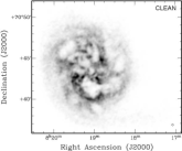
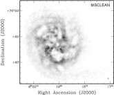
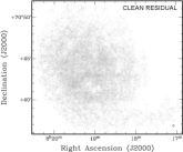
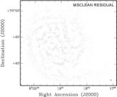
Figure 8.— clean (left) and msclean (right) integrated H i maps (top row) for Holmberg II. The maps were generated from the natural-weighted, masked, primary-beam corrected and for clean, residual flux corrected cubes. The equivalent residual integrated H i maps are also shown (bottom row). No primary-beam corrections and for clean, no residual flux corrections have been applied. The gray-scale levels run from $0$ to $500$ mJy beam^-1 km s^-1. Beams are marked in bottom right corner of images.

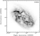
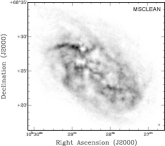
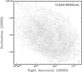
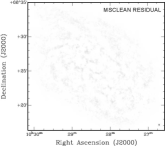
Figure 9.— clean (left) and msclean (right) integrated H i maps (top row) for IC 2574. The maps were generated from the natural-weighted, masked, primary-beam corrected and for clean, residual flux corrected cubes. The equivalent residual integrated H i maps are also shown (bottom row). No primary-beam corrections and for clean, no residual flux corrections have been applied. The gray-scale levels run from $0$ to $450$ mJy beam^-1 km s^-1. Beams are marked in bottom right corner of images.

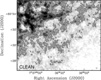
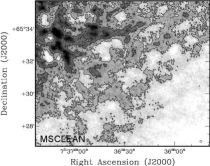
Figure 10.— Comparison of flux levels for NGC 2403. On the top is the clean integrated moment map and the bottom is the msclean version. Images were generated from the natural-weighted, masked and primary-beam corrected data. The clean image has been residual flux corrected. Contour levels of column density are plotted at $1\cdot 10^{21}$ and $2\cdot 10^{21}$ cm^-2. The gray-scale levels run from $0$ to $200$ mJy beam^-1 km s^-1. Beams are marked in bottom right corner of images.

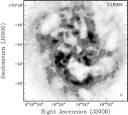
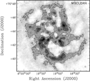
Figure 11.— Comparison of flux levels for Holmberg II. On the top is the clean integrated moment map and the bottom is the msclean version. Images were generated from the natural-weighted, masked and primary-beam corrected data. The clean image has been residual flux corrected. Contour levels of column density are plotted at $1\cdot 10^{21}$ and $2\cdot 10^{21}$ cm^-2. The gray-scale levels run from $0$ to $500$ mJy beam^-1 km s^-1. Beams are marked in bottom right corner of images.

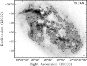
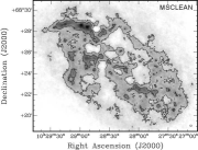
Figure 12.— Comparison of flux levels for IC 2574. On the top is the clean integrated moment map and the bottom is the msclean version. Images were generated from the natural-weighted, masked and primary-beam corrected data. The clean image has been residual flux corrected. Contour levels of column density are plotted at $1\cdot 10^{21}$ and $2\cdot 10^{21}$ cm^-2. The gray-scale levels run from $0$ to $450$ mJy beam^-1 km s^-1. Beams are marked in bottom right corner of images.

3.6. Flux and Noise Measurements

Table 2 shows the comparison of total flux for both weightings for the clean and msclean data. The total flux for the msclean data was calculated from the masked cubes after primary-beam correction, using the stat task of the GIPSY software package. The total flux values for the clean data are derived with the same method, using the primary-beam corrected data with residual-scaling applied. The uncertainties in the flux densities measured here is of the same order as the flux calibration ($\sim 10$%, see Walter et al. 2008). From Table 2, in all three galaxies it can be seen that msclean recovers more flux than classical clean for a given weighting. This is despite apparently higher peak fluxes for compact sources in the clean integrated H i maps of Figures 7 to 9. The flux gains by msclean are therefore mostly in the recovery the extended source structure. The relative differences in total fluxes as listed in Table 2 are consistent with the results derived by Cornwell (2008) using artificial data. Table 3 shows the rms noise values for both weightings. The noise was determined in line-free channels that were not used in determining the continuum.

Table 2Total flux comparison of clean and msclean for each galaxy.

Source	Weighting	Total Flux (Jy km s-1)
		NGC 2403	Holmberg II	IC 2574
clean	Natural	$1055$	$219$	$387$
	Robust	$977$	$210$	$363$
msclean	Natural	$1200$	$261$	$418$
	Robust	$1205$	$271$	$426$
Single-dish		$1172\pm 553$	$245\pm 54$	$466\pm 69$

Note. — The measurements for clean were made on data which had been residual flux corrected.

Table 3Noise level Comparison for clean (without residual-scaling) and msclean images.

Source	Weighting	Noise (mJy beam-1)
		NGC 2403	Holmberg II	IC 2574
clean	Natural	$0.38$	$0.92$	$0.56$
	Robust	$0.45$	$1.06$	$0.69$
msclean	Natural	$0.41$	$0.93$	$0.57$
	Robust	$0.50$	$1.11$	$0.68$

Note. — The measurements for clean were made on data which had not been residual flux corrected and all measurements were made in line-free channels that were not used in determining the continuum.

An important issue is whether the algorithms alter the amplitude or distribution of noise in the data in a significant way. Figure 13 shows histograms of the flux values in a channel that is free of galaxy emission and within an empty region of a channel containing galaxy emission. For clean, the non residual-scaled data has been used. For the noise in both emission and emission-free channels, and across both data-sets the noise has a Gaussian distribution. The noise in the empty channels of the msclean and clean data (left column) is identical. For channels containing emission there is a slight bias to negative values in the clean data, due to the clean bowl. We also note that there is a similar but smaller bias in the noise in the msclean emission channel. It is clear however, that neither algorithm alters the noise significantly.

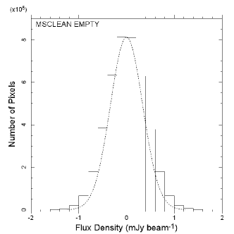
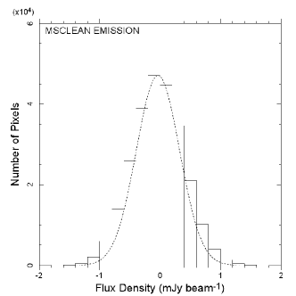
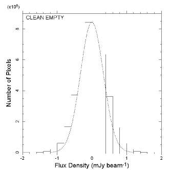
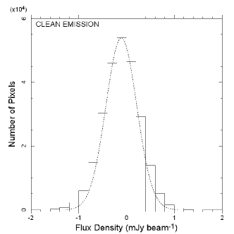
Figure 13.— Histograms of the flux density in the galaxy NGC 2403 for both msclean (top) and clean (bottom). On the left are histograms calculated an empty channel in the unmasked, non primary-beam corrected (and non residual-scaled for clean) data cube located at a heliocentric velocity of $278$ km s^-1. On the right are histograms calculated in a $500\times 500$ pixel box situated in an empty part of the channel containing galaxy emission at a heliocentric velocity of $201$ km s^-1. For each plot, $25$ bins of width $0.18$ mJy beam^-1 have been used. Also, for each histogram, the Gaussian fit to the histogram values has been plotted (dotted line).

3.6.1 Comparison to Single-dish Measurements

Ideally one would like to compare the derived flux values with total flux values derived using single-dish instruments. Unfortunately for the THINGS galaxies their large extent leads to single-dish measurements which are more uncertain than one would like. We list in Table 2 the single-dish fluxes derived by computing the average values and standard deviations of the single dish fluxes listed in the NASA/IPAC Extragalactic Database (NED). In general we see a good agreement, but a more precise comparison is precluded by the uncertainty in the single dish values. We also note there is a general satisfactory agreement between the fluxes derived here and those listed in Walter et al. (2008). Finally, we refer to Figure 4 in Walter & Brinks (1999) which plots the VLA H i (residual-corrected) spectrum for IC 2574 on top of a single-dish spectrum by Rots (1980) which shows excellent agreement.

3.7. H I Spectra

Figures 14, 15 and 16 show the flux density plotted as a function of velocity for NGC 2403, Holmberg II and IC 2574 respectively. The msclean natural (solid black line) and robust (dashed black line) result in higher flux densities than the standard clean natural (dotted gray line) and robust (dashed gray line) cubes. Additionally, msclean natural and robust weighting are equally good at recovering flux, whereas robust weighting is worse than natural weighting for clean. We also compare the residual flux density profiles of the two algorithms in Figure 17 for NGC 2403. For the clean algorithm, the residual profile has been corrected using both the dirty beam (i.e., residual flux scaling) and with the clean beam (without residual flux scaling). Because msclean cleans close to the noise level, there is essentially little source emission remaining in its residual profile in Figure 17 (gray solid line). On the other hand, the classical clean residual profile (long-dashed gray line) is a constant, flat line at a flux density of approximately $0.5$ Jy, showing that the algorithm has left source emission uncleaned (due to the flux cut-off used in the clean process). Correcting this residual profile using the clean beam leads to a significantly higher residual profile (gray short dashed line) that will result in erroneous flux measurements, as opposed to measurements using the same residual profile but corrected using the dirty beam (gray long dashed line).

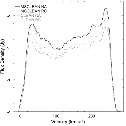
Figure 14.— Global H i Profile of NGC 2403 for both natural and robust clean and msclean cubes. The profiles are derived from masked, primary-beam corrected (and for clean, residual scaled) data.

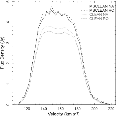
Figure 15.— Global H i Profile of Holmberg II for both natural and robust clean and msclean cubes. The profiles are derived from masked, primary-beam corrected (and for clean, residual scaled) data.

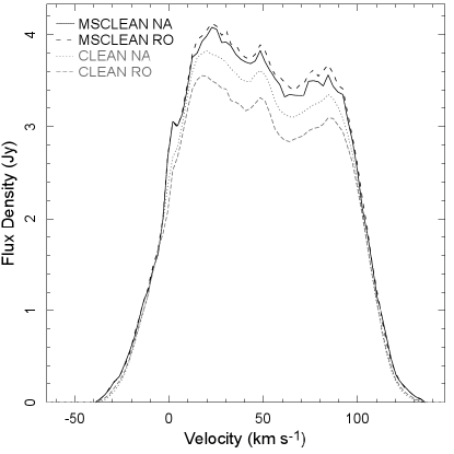
Figure 16.— Global H i Profile of IC 2574 for both natural and robust clean and msclean cubes. The profiles are derived from the masked, primary-beam corrected (and for clean, residual scaled) data.

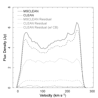
Figure 17.— Total (black) and residual (gray) H i flux profiles for the natural-weighted msclean (solid) and clean (long dashed) data cubes of NGC 2403. Also shown is the clean residual flux profile calculated using the clean beam (i.e., without residual flux scaling) as the short-dashed gray line. Total flux profiles are derived from the masked, primary-beam corrected (residual scaled for clean) data. Residual flux profiles are derived from masked, non primary-beam corrected data.

We also present a radial H i column density profile in Figure 18 for NGC 2403. The H i column density profile has been plotted for the clean data with and without residual flux scaling applied and for the msclean data. All profiles were generated using the ellint task in the MIRIAD software package, in $10$″ increments, correcting for the position angle and inclination of the H i disk. As can be seen, not applying residual flux scaling can lead to an overestimate of the H i flux (and thus column density) in the inner parts of the disk. As the disk radius increases, the non residual-scaled clean profile begins to equal the msclean and clean residual scaled profiles, then drops below the latter two profiles out to the extremes of the disk. There is therefore significant variations in the fluxes measured without residual-scaling the data. clean with residual-scaling applied agrees much more closely to msclean than when not applying residual scaling. The figure also demonstrates how msclean does not suffer as much from the clean bowl effect as classical clean and thus can probe the outer regions of the disk more effectively than classical clean. In the inner parts of the disk, the clean bowl is less significant because overlapping emission located at the same spatial position but different frequencies partly cancels its effect. In the outer parts of the disk, there are fewer overlapping flux regions, and so the bowl has a larger effect, depressing the flux in the clean profile. msclean on the other hand shows consistently higher H i column densities out to the extremes of the disk.

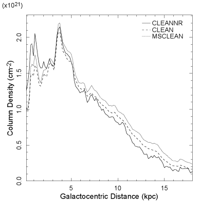
Figure 18.— The radial H i column density profile of the galaxy NGC 2403 for clean without residual scaling (solid line), clean with residual scaling (dashed line) and msclean (dotted line). The masked, primary-beam corrected data was used for the generation of the profiles.

3.8. Power Spectra

The integrated moment maps in figures 7, 8 and 9 seem to indicate that the msclean maps contain more small-scale structure than the clean maps. The difference between the msclean and clean maps can be quantified using the power spectrum of the resulting H i distributions in both types of maps. We derive the power (defined as the square of the modulus of the Fourier transform of the image) in azimuthally averaged rings with logarithmically increasing baseline length. Figure 19 shows the power spectra for our three sample galaxies for both sets of integrated H i maps. Both the clean and msclean spectra flatten sightly at large scales (i.e., shortest baselines), possibly indicating that some of these largest scales are not completely probed by the VLA, even at its shortest baselines. Alternatively it may indicate that these largest scales are simply not present in the galaxies under consideration. It is clear though that at large scales there is good agreement.

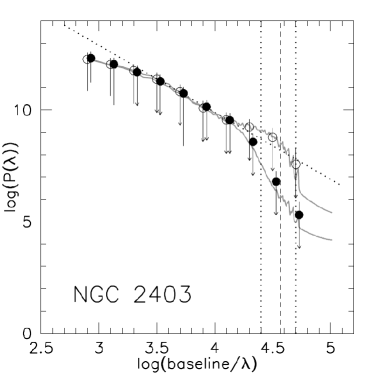
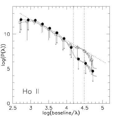
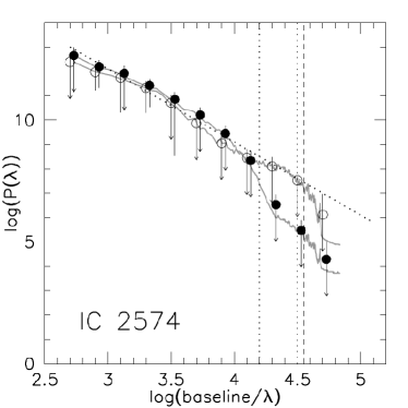
Figure 19.— Power spectra of the natural-weighted integrated H i maps. Filled circles show the standard clean data, open circles the msclean data. The points show logarithmically binned data, the thin gray lines show the actual behaviour of the power in linearly sampled intervals. The diagonal dotted line has a power law slope of $-3$. Note that it is not a fit to the data. The left-most dotted vertical line shows the natural-weighted beam size, the right-most dotted line half the natural-weighted beam size. The vertical dashed line shows the robust-weighted beam size. Arrows indicate that the lower error-bars extend beyond the plotted range.

As the spatial scale probed approaches the size of the natural-weighted beam however, the power in the clean integrated moment maps begins to decrease compared to the msclean maps. At about $\sim 1.5$ times the natural-weighted beam size we start to see a significant deviation. Also shown in Figure 19 is a power law with slope $-3$ which is a reasonable description for the power spectrum at intermediate scales. It is consistent with values found in other galaxies (Muller et al. 2004).

We will not attempt here to relate the power law slope to e.g., the turbulence or the energy input of the ISM, but we draw attention to the fact that as the small-scale power in the clean maps starts to fall away, the msclean power spectrum continues to follow this power-law behavior. This indicates that the msclean maps probe real small-scale structure more efficiently than the classical clean maps. Note that the power in the msclean maps only starts to drop away at scale sizes of half a natural-weighted beam. Scales probed in classical clean are only completely sampled down to $\sim 1.5$ times the natural-weighted beam size. Looking at Table 1 it can be seen that the robust beam sizes for IC 2574 and Holmberg II are about half the size of the natural beams. This means that msclean allows the probing of scales at close to robust-weighted resolution but with natural-weighted sensitivity, and at correct flux scales. This does not mean that msclean can super-resolve data, just that it is simply more efficient at extracting the small-scale information that is present in the data.

4. Multi-Scale, Multi-Resolution and Windowed CLEAN Comparisons

So far we have only explicitly compared msclean with classical clean. We now extend our comparisons to also include clean windows in combination with classical clean, and include the version of msclean implemented in AIPS. We refer to this algorithm as AIPS Multi-Resolution clean in keeping with the terminology used within the AIPS documentation. We note however, that it is not an implementation of the original multi-resolution clean (Wakker & Schwarz 1988) and so is similar in name only. The algorithm behind AIPS Multi-Resolution clean is the similar to the algorithm used by msclean. msclean and AIPS Multi-Resolution clean can therefore be thought of as differing implementations of the same scale-sensitive deconvolution algorithm.

A small variation on standard clean, which does not alter the algorithm in any way, is to define a clean ‘window’, restricting the clean processing to a defined area of the dirty map. The advantage of this windowed-clean is a greatly increased processing speed, particularly for extended sources. By defining a clean window, clean is restricted to where it can find components. However, care must be taken not to define a window that is too small to encompass low-level extended structure. Obviously, for the case of extended emission throughout a large fraction of the primary beam, the clean window has to become so large that a windowed-clean reverts to a simple un-windowed clean.

For these comparisons between the algorithms, we have used a channel map from Holmberg II located at heliocentric velocity $165$ km s^-1. For msclean and AIPS Multi-Resolution clean, six scales/resolutions were chosen, using the same method as described in Section 3.2. The diameters from smallest to largest were $0$″, $4$″, $13$″, $40$″, $133$″ and $400$″. A gain of $0.7$ was used for msclean and AIPS Multi-Resolution clean (the same gain as used for msclean before) while a gain of $0.1$ was used for the window clean (in line with the gain used in classical clean). For all algorithms, a flux threshold of $2.3$ mJy beam^-1 ($2.5\sigma$) was used in all algorithms. Maximum iteration limits of $5000$ were set for msclean and AIPS Multi-Resolution clean and $100000$ for the window clean. We note that for all algorithms the flux threshold was reached before hitting the iteration limit.

4.1. Beams, Total Flux and Noise Measurements

Values for the clean beams, total flux recovered and the rms noise can be found in Table 4. To measure the flux, a mask was created from the msclean restored image by blanking out all emission below a $2\sigma$ level and applying this mask to all the images. The resulting masked image was corrected for the primary beam and used to measure the flux. For clean and windowed-clean, residual-corrected images were used for measuring the total flux. For measuring the rms noise, unmasked, non primary beam corrected (and for clean with/without windows, non residual-scaled) images were used. The rms noise was measured in a $50\times 50$ pixel box within the cleaned region of each image, and in a location with no source emission.

Table 4Beam, Total Flux and rms Noise comparison for msclean, AIPS Multi-Resolution clean, windowed-clean and clean in Holmberg II.

Algorithm	Beam Size	Flux Recovered	rms Noise
	($\arcsec$)	(Jy)	(mJy beam-1)
msclean	$11.3\times 10.8$	$3.11$	$0.83$
AIPS Multi-Resolution clean	$13.7\times 12.6$	$3.02$	$0.87$
clean	$13.7\times 12.6$	$2.77$	$0.88$
Windowed-clean	$13.7\times 12.6$	$2.88$	$0.91$
Windowed-clean ($1\sigma$)	$13.7\times 12.6$	$2.93$	$1.3$
Windowed-clean ($0.5\sigma$)	$13.7\times 12.6$	$2.95$	$1.6$

Note. — Total flux measurements for clean and windowed-clean were made with data that was residual flux corrected, while rms noise measurements were made with data which was not residual flux corrected.

Windowed-clean recovers $\sim 5$% more flux than clean, but does not recover as much flux as the two scale-sensitive algorithms. The number of iterations taken for each to reach the flux threshold were $3500$ for msclean, $4050$ for AIPS Multi-Resolution clean, $5100$ for windowed-clean and $9720$ for clean. The flux gains made here on real data by the scale-sensitive algorithms are in line with the gains made by these algorithms on simulated data (Cornwell 2008). The rms noise measurements are in good agreement, which indicates that none of the algorithms significantly changes the noise properties of the data. We note that the small differences in noise levels between those listed in Table 4 (as derived for Holmberg II using msclean, AIPS Multi-Resolution clean and clean) are slightly different from those listed in Table 3 (as determined for a line-free channel in the Holmberg II data cube). This difference is mostly attributable to small channel-to-channel changes in the average noise level, as well as small statistical spatial noise fluctuations in each channel. We find these noise measurements to have a dispersion of $\sim 0.03$ mJy for this particular case.

When using clean windows, the search for clean components is restricted to the area of known flux (i.e., the window) and it should therefore in principle be possible to clean to a deeper level, thus increasingly negating the need for residual scaling. We have tested this by running windowed-clean down to additional flux thresholds of $1\sigma$ and $0.5\sigma$ in Holmberg II. The total flux recovered and the rms noise are listed in Table 4. We note there is a significant increase in the number of iterations required to clean down to these flux thresholds, with a marginal gain in recovered flux. For a $1\sigma$ threshold, $38000$ iterations are required and for a $0.5\sigma$ level, $198000$ iterations are needed. For the original $2.5\sigma$ threshold, $5000$ iterations were required. In comparison, msclean and AIPS Multi-Resolution clean recover more flux without an increase in rms noise, and with fewer iterations.

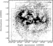
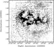
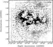
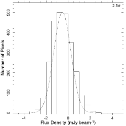
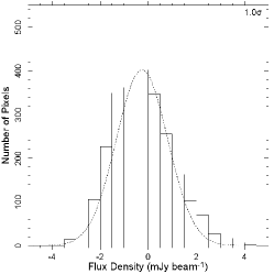
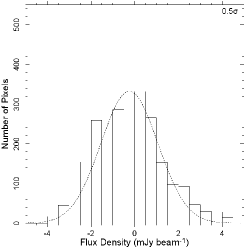
Figure 20.— Images (top row) of windowed-clean to $2.5\sigma$ (left), $1\sigma$ (middle) and $0.5\sigma$ (right) for a channel for the galaxy Holmberg II data. The outline of the window used is shown in black. Images are residual flux corrected, unmasked and without primary-beam correction applied. The gray-scale levels run from $0$ to $8$ mJy beam^-1. Also shown are histograms (and the Gaussian fit) of the flux values (bottom row). The histogram values are sampled in a $50\times 50$ pixel box within the cleaned region and where there is no source emission. Images without residual scaling applied were used for the histogram generation.

The resulting channel maps along with the channel map for the original windowed-clean to $2.5\sigma$ flux threshold are shown in Figure 20. The window applied is marked by the black box around the emission in the images. The box was chosen based on emission visible in the dirty image. After deconvolution, additional emission became visible outside our clean window (as shown in Figure 20). Normally one would adjust the clean window and perform further clean runs. Here, however, we only show the result from our first run, as this clearly illustrates the differences in noise properties inside and outside the clean box. Immediately noticeable in these images is the increased ‘spottiness’ that comes with cleaning to a deeper flux level. This is most likely due to clean operating into the noise and thus cleaning noise spikes as opposed to real emission with a distortion of the noise. This can be seen in the histograms of Figure 20 which show the increased rms noise for the deepest windowed-cleans and is also clear from the measured rms listed in Table 4. The same negative bias as observed in Figure 13 is seen in the histogram of the windowed-clean down to a flux threshold of $2.5\sigma$ (left histogram), but this bias disappears for deep windowed-cleans (middle and right histograms). A deep windowed-clean can therefore eliminate the negative bowl, but does so at the cost of distorted (and increased) noise. These results are in line with those on simulated data by Cornwell (2008).

We note that the definition of a clean window is trivial for the case of a single channel map discussed here. For a large data-cube of a complicated extended source, an individual clean window would need to be defined for each channel of the cube, as the structure of the source in each channel changes in both shape and position. It is therefore impractical to use windowed-clean for the THINGS sample, where the number of spectral channels for a single galaxy can be as high as $100$.

4.2. Channel Map Comparison

In Figure 21, we compare the images produced by each algorithm. From top to bottom in each figure are the images for msclean, AIPS Multi-Resolution clean, windowed-clean and clean. The left column is the restored image. The center column is the restored image smoothed to $30$″ with a contour plotted at level equal to $-1.5\sigma$ of the (smoothed) noise to show the effect of the negative bowl. The right column is the residual image. For each column, all of the images are plotted to the same gray-scale levels. Data without masks and not corrected for primary-beam attenuation was used. For clean and windowed-clean, no residual scaling was applied. The contours in the smoothed images (middle column) show that the clean bowl is notably less present for the msclean and AIPS Multi-Resolution clean images. There is also no trace of emission in the residual images for these two algorithms (right column), while both windowed and un-windowed clean leave an obvious pedestal.

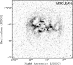
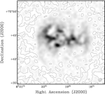
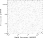
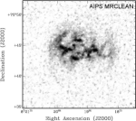
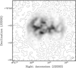
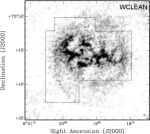
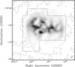
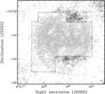
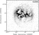
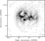
Figure 21.— The cleaned image (left), smoothed to $30$″ (middle) and residual (right) maps for, from top row to bottom row, msclean, AIPS Multi-Resolution clean, windowed-clean and clean, for the galaxy Holmberg II. Images are un-masked and no primary-beam correction has been applied. No residual-scaling has been applied to the clean and windowed-clean images. Restoring beams are as marked in the bottom-right corner of each image. For each image in the center column, a (smoothed) contour has been plotted at a flux density level of $-0.45$ mJy beam^-1 ($-1.5\sigma$ of the clean noise). For the windowed-clean images and residual, the outline of the window used is also shown in black. The gray-scale levels for the left and right columns run from $0$ to $15$ mJy beam^-1and for the middle column, $0$ to $70$ mJy beam^-1.

4.3. Difference Maps

The variations on clean discussed here all use the same principles, but different implementations to produce a final image. It is therefore interesting to see whether these different methods introduce differences in the final images. To that end, difference images of msclean and AIPS Multi-Resolution clean minus clean/windowed-clean have been constructed. A difference image of the two scale-sensitive algorithms, msclean minus AIPS Multi-Resolution clean, was also made to compare the relative difference between each. All of these images were generated by performing a pixel-by-pixel subtraction of two restored images. The resulting images are shown in Figures 22 and 23. Subtractions for residual-scaled and non residual-scaled clean are shown. The former has all flux below $2\sigma$ masked, as the comparison is only valid in regions where there is source emission. Similarly for windowed-clean, only the difference within the window is shown. The differences in the noise are shown for the non-residual scaled clean subtractions. Also shown are histograms of the flux values in each difference image. The histograms were calculated within the same region of each image, which was equal to the window used for windowed-clean.

The difference between the clean and windowed-clean subtractions for either msclean or AIPS Multi-Resolution clean is minimal. This is expected, as the only difference is the application of a clean window. The only major differences in subtractions of msclean and AIPS Multi-Resolution clean minus classical clean are directly around and at the location of the source emission. Negative peaks in these difference images correspond to locations of maximum source emission in the actual images. The AIPS Multi-Resolution clean minus clean/windowed-clean difference images in Figure 23 also show additional positive difference flux around the negative peaks.

Looking at the difference image of msclean minus AIPS Multi-Resolution clean in Figure 22, these locations show an average zero difference flux. Overall, this difference image shows little correlation with the source structure. The small peaks of negative difference flux visible in the image do appear to be at locations of strong source emission as is the case for each scale-sensitive algorithm minus classical clean, but the extent of such differences is much smaller than in the latter difference images. Both scale-sensitive algorithms are therefore performing a similar clean process (i.e., choosing components of similar strength size and location). But where there is compact, high peak flux emission present, the scale-sensitive algorithms and classical clean diverge in their processing techniques. This difference leads to greater total flux recovery for scale-sensitive algorithms, as shown in the previous sections.

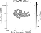
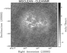
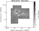
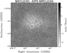
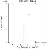
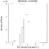
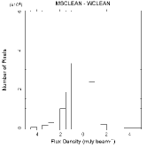
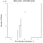
Figure 22.— Difference images (top row) of msclean minus residual-scaled clean, non residual-scaled clean, residual-scaled windowed-clean and AIPS Multi-Resolution clean for Holmberg II. The original images were corrected for the primary-beam. For residual-scaled clean all flux below $2\sigma$ of the rms noise in the msclean restored image has been masked. For windowed-clean, only the difference within the clean window used is shown. Histograms (bottom row) of the flux values calculated within the same area of each image and equal to the area inside the window used for the windowed-clean are also shown. Gray-scale levels in the images run from $-5$ to $5$ mJy beam^-1.

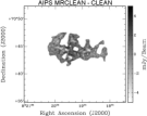
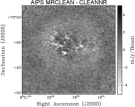
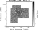
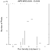
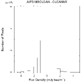
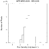
Figure 23.— Difference images (top row) of AIPS Multi-Resolution clean minus residual-scaled clean, non residual-scaled clean and residual-scaled windowed-clean for Holmberg II. The original images were corrected for the primary-beam. For residual-scaled clean all flux below $2\sigma$ of the rms noise in the msclean restored image has been masked. For windowed-clean, only the difference within the clean window used is shown. Histograms (bottom row) of the flux values calculated within the same area of each image and equal to the area inside the window used for the windowed-clean are also shown. Gray-scale levels in the images run from $-5$ to $5$ mJy beam^-1.

5. Applications of MSCLEAN

Having performed and discussed the comparison of msclean against clean and other algorithms the remainder of this paper is on some real-world applications of msclean. We focus on two particular applications that relate to small-scale extended structure in the H i gas of galaxies. In Section 5.1, the application of msclean to helping the search for H i holes in the disk of galaxies is discussed, while in Section 5.2, and initial attempt is made to apply the increased contrast provided by msclean to the study of faint, anomalous H i gas structures outside of the galactic disk.

5.1. H I Holes

High resolution H i imaging has revealed a deeper level of structure in the inter-stellar medium that forms an intricate tapestry of holes, shells and bubbles that permeate and define a complex set of tunnels, networks and cavities of under-densities through the tenuous interstellar medium (e.g., Brand & Zealey 1975; Heiles 1979; McCray & Snow 1979; Brinks & Bajaja 1986; Deul & den Hartog 1990; Kim et al. 1999; Stanimirovic et al. 1999; Walter & Brinks 1999). Such small-scale structures provide an excellent environment in which to compare msclean to clean. Here we compare the results of a search for holes in the THINGS and msclean cubes of the same galaxy.

To inspect the cubes and integrated moment maps, the KARMA software suite of visualization tools was used (Gooch 1996). In particular, the kvis and kpvslice tools were extensively used for finding the holes. These two tools provide two different ways of looking at the H i cube. The former provides views of the spatial and spectral planes in the data cube. The latter allows arbitrary position-velocity slices through the cube to be made, providing an alternative view of a part of the disk. To find a hole, a search was first conducted in kvis for under-densities in sequential velocity channels. Then, using kpvslice, a position-velocity ($pV$) cut through the hole was taken and the hole was classified as one of three different types by observing its profile.

The qualities that define a hole from an under-density in the H i gas are somewhat subjective and depend on the signal-to-noise of their feature. In this study, low signal-to-noise features that were of the order of the size of the beam were generally classified as just noise. A structure had to exist in more than four velocity channels as well before considering it. To verify the reliability of the method of identification genuine, a double-blind test was conducted. This involved searching for holes in a single galaxy using the same technique for both the clean and msclean data, and by two different people. Only the basic observed properties of the hole candidates were cataloged in the test, being the position, size and shape of each hole. Also a ‘quality rating’ between one and ten was assigned. The quality rating defined the confidence that the observer thought a candidate hole was a genuine structure. So a quality rating of $7$ meant that the observer was $70\%$ confident that the candidate was real. The end result of the double blind test was four catalogs, two for each observer and imaging algorithm.

There were significant variations between the catalogs of the two observers in both the clean and msclean data. However, the agreement between the catalogs, both as regards to size and shape of the holes increased with increasing quality rating. This is shown in Figure 24 where the ellipses fitted to various holes are shown for progressively higher quality ratings. It was found, and as shown in the figure, that at around a quality value of $6$, there was good agreement between the observers. That is, with the search method and criteria used in this paper, all candidates found with a quality rating of $6$ or above are believed to be real holes.

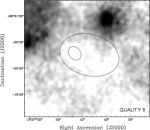
Figure 24.— Comparison of the agreement bewteen hole sizes and shapes with progressively higher quality ratings for the msclean catalogs created in the double-blind test. The quality ratings increase from $5$ to $7$ from left to right. The gray-scale levels run from $15$ to $260$ mJy beam^-1 km s^-1.

The final hole catalog overlays for the clean and msclean data on an msclean natural-weighted integrated intensity map is shown in Figure 25. Comparison of the overlays shows the physical implications of the results discussed in the previous sections. Inspection of the msclean hole overlay appears to show an excess of small holes, especially in the inner disk. Figure 26 shows a histogram of the derived diameters of holes in both the clean (dashed) and msclean (solid) catalogs. The difference is indicative of the extra contrast provided by msclean. Without the smoother background of the clean residual pedestal, structures are better defined and with a higher contrast. Whether this extra population of small holes is related to, e.g., star-formation events, or whether we are observing small scale turbulence, or as yet unrecognized systematic effects is beyond the scope of this paper.

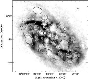
Figure 25.— msclean integrated H i map with hole catalog overlays created from msclean (black) and clean (white) data. The gray-scale levels run from $0$ to $251$ mJy beam^-1 km s^-1.

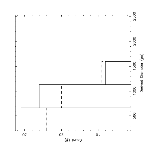
Figure 26.— Histogram of the derived diameters of holes in the clean (dashed histogram) and msclean (solid histogram) hole catalogs of the galaxy IC 2574.

5.2. Anomalous Gas

Increased resolution in radio images has also led to interesting results beyond the high surface brightness disk of galaxies. ‘Anomalous’ neutral gas structures have been detected in a few nearby galaxies such as NGC 891 (Swaters et al. 1997) and including NGC 2403 (Fraternali et al. 2002). It has only been in recent, deep H i observations that these structures have been revealed as being linked to a cold gaseous halo well above the main disk (Oosterloo et al. 2007). Like holes, such structures require significant angular resolution for detection. And unlike holes, their location is mostly within a region where clean characteristics may play an important role in the interpretation of the data.

In this study, a comparison of the structures described in Fraternali et al. (2002) was made in the clean and msclean data sets. The KARMA software package was employed to make $pV$ slices and channel map images as outlined in Section 5.1. The structure located at $\sim 108$ km s^-1 by Fraternali et al. (2002) is easily observed in both data-sets as shown in Figure 27. The effects of the clean bowl are also clearly visible in the clean image as an apparent decrease in the noise level. This has a negative impact on the visibility of fine structure, however, in a $pV$ slice taken across the major axis of the ellipse as shown in Figure 28. A lot of the structure is hidden by the bowl, and much extra analysis would be needed to quantify structures over the entire cube to the same quantitative levels. In contrast, the msclean image has a flat background and more features of the structure are visible. It is clear that a more detailed search will need to be conducted in NGC 2403. But as indicated, msclean greatly enhances the visibility of structures near the disk.

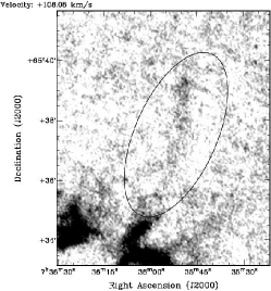
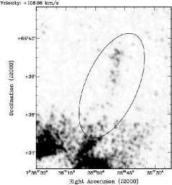
Figure 27.— Zoomed in channel map for NGC 2403 for both msclean (left) and clean (right) data cubes. Shown within the ellipse is the ‘anomalous’ H i structure as discovered by Fraternali et al. (2002). The gray-scale levels run from $0$ to $15$ mJy beam^-1.

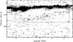
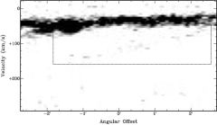
Figure 28.— Position-velocity ($pV$) cuts through the major axis of the ellipse around the structure observed in Figure 27 in the msclean (top) and clean (bottom) natural-weighted data cubes. The gray-scale levels run from $0.2$ to $2$ mJy beam^-1.

6. Summary

This paper presents a demonstration of the Multi-Scale clean algorithm on a sample of galaxies from THINGS. msclean is an extension of clean that attempts to overcome some of the short-comings of the latter algorithm, particularly relating to extended sources such as galaxies. The THINGS data are well-suited to test and compare the performance of clean and msclean. A summary of the important results follows.

1. msclean (which we here take to explicitly include both the CASA as well as the AIPS Multi-Resolution clean implementations) uses fewer iterations than classical clean and can clean down to a low flux threshold much more efficiently than the latter. The algorithm itself is also relatively simple and easy to implement and is currently available in the CASA and AIPS software packages.

2. msclean removes the bowl and pedestal characteristics that occur when clean is applied to extended sources. In the clean data the extended wings of the dirty beam that are left uncleaned in the pedestal smooth out a lot of the low-level fine-scale structure. msclean, by significantly reducing the pedestal, reveals this structure more clearly. This leads to better contrast and higher resolution at the lowest flux levels. The clean bowl lowers the apparent flux of all structures within it, due to the negative background it creates. Extended structure usually has a low column density compared to compact structure and so the effect is more pronounced for extended structure. msclean can greatly reduce this bowl effect, thereby better recovering large-scale structure. The noise characteristics of the final cubes remain the same.

3. msclean illustrates the importance for residual flux scaling when using classical clean. This need for residual flux scaling arises because classical clean cleans down to a set flux level, leaving a residual map which is characterized by the dirty beam. The flux in the residuals has to be rescaled by the ratio of the clean beam over the dirty beam area before restoring the clean components back on the residual map. msclean does a better job in modeling the emission, leaving virtually no residual and hence removing the need for such scaling.

4. The added contrast provided by msclean is useful for a number of astronomical problems involving small-scale structure. This paper has highlighted two such problems; H i holes in the disk and anomalous gas in the halo of nearby galaxies. Comparison of hole catalogs made for the clean and msclean data-sets shows that msclean reveals finer structure in the central disk by removing the artificial smoothness associated with clean. A comparison of a known anomalous gas structure in NGC 2403 demonstrated that the removal of the clean bowl by msclean better reveals structure outside of the disk as well.

References

- Bhatnagar & Cornwell (2003) Bhatnagar, S., & Cornwell, T. J. 2003, in Presented at the Society of Photo-Optical Instrumentation Engineers (SPIE) Conference, Vol. 5169, Astronomical Adaptive Optics Systems and Applications. Edited by Tyson, Robert K.; Lloyd-Hart, Michael. Proceedings of the SPIE, Volume 5169, pp. 331-340 (2003)., ed. R. K. Tyson & M. Lloyd-Hart, 331–340
- Bhatnagar & Cornwell (2004) Bhatnagar, S., & Cornwell, T. J. 2004, A&A, 426, 747, arXiv:astro-ph/0407225
- Brand & Zealey (1975) Brand, P. W. J. L., & Zealey, W. J. 1975, A&A, 38, 363
- Briggs (1995) Briggs, D. S. 1995, in Bulletin of the American Astronomical Society, Vol. 27, Bulletin of the American Astronomical Society, 1444
- Brinks & Bajaja (1986) Brinks, E., & Bajaja, E. 1986, A&A, 169, 14
- Brinks & Shane (1984) Brinks, E., & Shane, W. W. 1984, A&AS, 55, 179
- Clark (1980) Clark, B. G. 1980, A&A, 89, 377
- Cornwell et al. (1999) Cornwell, T., Braun, R., & Briggs, D. S. 1999, in Astronomical Society of the Pacific Conference Series, Vol. 180, Synthesis Imaging in Radio Astronomy II, ed. G. B. Taylor, C. L. Carilli, & R. A. Perley, 151
- Cornwell (2008) Cornwell, T. J. 2008, ArXiv e-prints, 806, arXiv:astro-ph/0806.2228
- Deul & den Hartog (1990) Deul, E. R., & den Hartog, R. H. 1990, A&A, 229, 362
- Fraternali et al. (2002) Fraternali, F., van Moorsel, G., Sancisi, R., & Oosterloo, T. 2002, AJ, 123, 3124, astro-ph/0203405
- Glazebrook & Economou (1997) Glazebrook, K., & Economou, F. 1997, The Perl Journal, 5
- Gooch (1996) Gooch, R. 1996, in ASP Conf. Ser. 101: Astronomical Data Analysis Software and Systems V, ed. G. H. Jacoby & J. Barnes, 80
- Heiles (1979) Heiles, C. 1979, ApJ, 229, 533
- Högbom (1974) Högbom, J. A. 1974, A&AS, 15, 417
- Jörsäter & van Moorsel (1995) Jörsäter, S., & van Moorsel, G. A. 1995, AJ, 110, 2037
- Kim et al. (1999) Kim, S., Dopita, M. A., Staveley-Smith, L., & Bessell, M. S. 1999, AJ, 118, 2797
- McCray & Snow (1979) McCray, R., & Snow, Jr., T. P. 1979, ARA&A, 17, 213
- Muller et al. (2004) Muller, E., Stanimirović, S., Rosolowsky, E., & Staveley-Smith, L. 2004, ApJ, 616, 845, arXiv:astro-ph/0408259
- Oosterloo et al. (2007) Oosterloo, T., Fraternali, F., & Sancisi, R. 2007, Astronomical Journal, 134, 1019, arXiv:0705.4034
- Rots (1980) Rots, A. H. 1980, A&AS, 41, 189
- Schwab (1984) Schwab, F. R. 1984, AJ, 89, 1076
- Schwarz (1978) Schwarz, U. J. 1978, A&A, 65, 345
- Stanimirovic et al. (1999) Stanimirovic, S., Staveley-Smith, L., Dickey, J. M., Sault, R. J., & Snowden, S. L. 1999, MNRAS, 302, 417
- Starck et al. (1994) Starck, J.-L., Bijaoui, A., Lopez, B., & Perrier, C. 1994, A&A, 283, 349
- Starck et al. (2002) Starck, J. L., Pantin, E., & Murtagh, F. 2002, PASP, 114, 1051
- Swaters et al. (1997) Swaters, R. A., Sancisi, R., & van der Hulst, J. M. 1997, ApJ, 491, 140, arXiv:astro-ph/9707150
- Tan (1986) Tan, S. M. 1986, MNRAS, 220, 971
- Thompson et al. (2001) Thompson, A. R., Moran, J. M., & Swenson, Jr., G. W. 2001, Interferometry and Synthesis in Radio Astronomy, 2nd Edition (Interferometry and synthesis in radio astronomy by A. Richard Thompson, James M. Moran, and George W. Swenson, Jr. 2nd ed. New York : Wiley, c2001.xxiii, 692 p. : ill. ; 25 cm. ”A Wiley-Interscience publication.” Includes bibliographical references and indexes. ISBN : 0471254924)
- Wakker & Schwarz (1988) Wakker, B. P., & Schwarz, U. J. 1988, A&A, 200, 312
- Walter & Brinks (1999) Walter, F., & Brinks, E. 1999, AJ, 118, 273
- Walter et al. (2008) Walter, F., Brinks, E., de Blok, W. J. G., Bigiel, F., Kennicutt, R. C., Jr., Thornley, M. D., & Leroy, A. K. 2008, AJ, arXiv:astro-ph/0810.2125