The relation between stellar mass and weak lensing signal around galaxies: Implications for MOND

Abstract

We study the amplitude of the weak gravitational lensing signal as a function of stellar mass around a sample of relatively isolated galaxies. This selection of lenses simplifies the interpretation of the observations, which consist of data from the Red-sequence Cluster Survey and the Sloan Digital Sky Survey. We find that the amplitude of the lensing signal as a function of stellar mass is well described by a power law with a best fit slope $\alpha=0.74\pm 0.08$. This result is inconsistent with Modified Newtonian Dynamics, which predicts $\alpha=0.5$ (we find $\alpha>0.5$ with 99.7% confidence). As a related test, we determine the MOND mass-to-light ratio as a function of luminosity. Our results require dark matter for the most luminous galaxies ($L\mathrel{\raise 1.29167pt\hbox{$>$\kern-7.5pt\lower 4.30554pt\hbox{$\sim$}}}10^{11}L_{\odot}$). We rule out an extended halo of gas or active neutrinos as a way of reconciling our findings with MOND. Although we focus on a single alternative gravity model, we note that our results provide an important test for any alternative theory of gravity.

1 Introduction

It is now well established that there are significant discrepancies between the Newtonian gravitational mass and the observable luminous mass on scales ranging from galaxies to clusters of galaxies. Two fundamentally different explanations have been proposed to solve these observations. The current paradigm is that General Relativity (GR) is correct on large scales, but that the derived gravitational mass is larger because of large amounts of unseen matter. This has led to the current standard cosmological model of a universe dominated by Cold Dark Matter and a cosmological constant ($\Lambda$CDM). This model is well-developed and widely applied to galactic and cosmological observations. It fits a range of observations, most notably the cosmic background radiation, extremely well (e.g., Spergel et al. 2007). The need for dark matter to explain astronomical observations has been a long-standing issue and a number of dark matter candidates, inspired by particle physics, have been suggested.

The current lack of a direct detection of the dark matter particle has led to an alternative approach to explain the observations. Instead of invoking dark matter, it is assumed that the law of gravity differs from the Newtonian gravity on a scale of weak gravity which cannot yet be reproduced in current gravitational experiments. One of the most studied alternatives is Modified Newtonian Dynamics (MOND) proposed by Milgrom (1983a). It has evolved over the past 25 years from an empirical fit to galaxy rotation curve data (Milgrom 1983b, Sanders & McGaugh 2002) to a relativistic tensor-vector-scalar theory (TeVeS, Bekenstein 2004). Recent developments include a theory of a vector field with a non-linear coupling to the space-time metric (Zlosnik, Ferreira, Starkman 2007, Zhao 2007).

MOND works particularly well on galactic scales (for a review, see Sanders & McGaugh 2002) and this is where most (dynamical) tests have focused on (e.g. Read & Moore 2005, Famaey et al 2006, Nipoti et al 2007, Corbelli & Salucci 2006, Gentile et al. 2007, Zhao & Famaey 2006, Famaey & Binney 2005). There are a few tests on sub-galactic scales using the velocity dispersion of globular clusters (Baumgardt et al. 2005) and using the tidal radius (Zhao 2005, Zhao & Tian 2006).

Our approach differs from previous studies in a number of ways. Unlike GR, MOND is a non-linear gravity theory, resulting in fundamental differences in their global scaling relations. Hence, rather than comparing the strength of the gravitational potential, we focus on how it changes with (baryonic) mass, although we do consider an example of the former as well. A fundamental property of MOND is its ‘prediction’ of a Tully-Fisher relation (Tully & Fisher 1977). In MOND this relation follows from the theory (Milgrom 1983b), whereas in $\Lambda$CDM it arises from the interplay between dark and baryonic matter. Also note that observationally the Tully-Fisher relation is one between the luminosity and the (maximum) rotation velocity, and thus is a test on sub-galactic scales.

It is therefore useful to examine MOND on scales much larger than those probed by rotation curves. Probing the gravitational potential in these outer regions of galaxies provides an ideal test of alternative gravity, because of the absence of luminous matter (except for a few satellites and globular clusters). It is in these regions where MOND and $\Lambda$CDM differ most markedly. In the dark matter paradigm we would call these regions ‘dark matter dominated’ and in MOND we call them ‘deep-MOND regions’. Finally, rather than dynamics, we will study the weak gravitational lensing signal around galaxies. We refer the interested reader to Hoekstra & Jain (2008) for a recent review on weak lensing.

We note that other tests involving (strong) gravitational lensing already have provided important constraints, albeit on relatively small scales. These studies typically reveal a factor of two discrepancy between stellar mass and the lensing mass using MOND (Zhao, Bacon, Taylor, Horne 2006, Chen & Zhao 2006, Angus et al. 2007a, Takahashi & Chiba 2007, Ferreras et al. 2007, Natarajan & Zhao 2008). Of particular intestest is the weak gravitational lensing study by Clowe et al. (2006) of the ‘Bullet’ cluster. Clowe et al. (2006) found a large offset between the matter distribution, as inferred from the lensing analysis, and the gas (which contains most of of the baryonic mass). The lensing map, however, does agree well with the distribution of galaxies, which is expected if both the dark matter and stars in galaxies are collisionless.

To probe the outer regions around galaxies we employ a technique called weak gravitational galaxy-galaxy lensing (hereafter g-g lensing), which is the statistical study of the deformation of distant galaxies by foreground galaxies. Since the gravitational distortions induced by an individual lens are too small to be detected, one has to resort to the study of the ensemble averaged signal around a large number of lenses. Of particular interest is that the g-g lensing signal can be measured out to large projected distance, where dynamical methods are of limited use due to the lack of luminous tracers. Hence, g-g lensing provides a unique and powerful tool to probe the gravitational potential on large scales. Only studies of satellite galaxies can also probe these regions (e.g., Zaritsky & White 1994; McKay et al. 2002; Prada et al. 2003; Conroy et al. 2007).

Since the first detection by Brainerd et al. (1996), the accuracy of g-g lensing studies has improved dramatically thanks to improved analysis techniques and large amounts of wide-field imaging data (e.g. Fischer et al. 2000, Hoekstra et al. 2004, Hoekstra et al. 2005, Mandelbaum et al. 2006, Parker et al. 2007). We refer to these papers for a more in-depth discussion of this area of research. Relevant for our study is the availability of (photometric or spectroscopic) redshift information for the lens galaxies. Only recently has this kind of information become available for large samples (Hoekstra et al. 2005, Mandelbaum et al. 2006). As a result we can now compare how the strength of the g-g lensing signal depends on the baryonic content of the lenses.

This paper is organized as follows. In §2, we discuss the expected dependence of the lensing signal on stellar mass. In §3 we describe the galaxy-galaxy lensing data used in our analysis. In §4 we present our results and discuss the implications for MOND. Throughout this paper, we adopt a Hubble parameter $H_{0}=70$ km/s/Mpc and all the error bars correspond to 68% confidence limits ($1\sigma$).

Figure 1: The observed ensemble averaged tangential shear around ‘isolated’ galaxies from Hoekstra et al. (2005). The data are shown for 7 luminosity bins (with the mean $L_{R}$ indicated in units of $10^{9}L_{R,\odot}$). The solid line indicates the best fit MOND point mass model. The lensing signal has been scaled to that of a lens at the average lens redshift ($z\sim 0.32$) and a source redshift of infinity.

2 Theoretical Predictions

One of the reasons for the success of MOND is the ability to provide excellent fits to rotation curves over a wide range in mass, thanks to its ‘built-in’ Tully-Fisher relation (Milgrom 1983b). As we show below, this feature has consequences for the predicted scaling of the lensing signal with stellar mass.

In MOND the only source of gravity is the luminous matter. As we are concerned with the lensing signal on large scales, we assume that the galaxy (stellar) mass distribution can be approximated by a point mass model. We have verified that the lensing signal on large scales ($>20$ kpc) is insensitive to the actual baryonic density profile. This is expected because the shear at large radii depends on the enclosed mass, which quickly converges to the same value for sufficiently compact mass distributions. Under these assumptions the MOND effective density $\rho_{\rm eff}$ for a point mass with mass $M$ is given by (see the Appendix for a discussion of the calculation for spherically symmetric mass distributions):

$$\rho_{\rm eff}(r)=\frac{\nabla^{2}\Phi}{4\pi G}=\frac{v_{0}^{2}}{4\pi G}\frac{1}{r^{2}},$$ (1)

where $\Phi$ is the gravitational potential in MOND, $v_{0}\equiv{(GMa_{0})}^{\frac{1}{4}}$ and $a_{0}$ is the MOND critical acceleration ($a_{0}\approx 10^{-8}$cms^-2). We assumed that $r\gg r_{0}\equiv\sqrt{GM/a_{0}}$. For a mass $M=10^{11}M_{\odot}$, we find $r_{0}\approx 10$kpc, which is much smaller than the scales we probe in this paper. Once we have obtained the effective density $\rho_{\rm eff}$, we can apply the same procedure as in the GR case to calculate the tangential shear (Zhao, 2006). The effective surface density is given by

$$\Sigma(r)=\frac{v_{0}^{2}}{4G}\frac{1}{r}.$$ (2)

The convergence $\kappa$ is the ratio of the surface density and the critical surface density $\Sigma_{\rm crit}$, which is given by

$$\Sigma_{\rm crit}=\frac{c^{2}}{4\pi G}\frac{D_{s}}{D_{l}D_{ls}},$$ (3)

where $D_{ls}$ is the distance from the lens to the source and $D_{l}$ and $D_{s}$ are the distances from the observer to the lens and the source, respectively. We use the fact that the azimuthally averaged tangential shear $\gamma_{t}$ (which corresponds to the observed g-g lensing signal) is related to the convergence through $\gamma_{t}={\bar{\kappa}(<r)}-\kappa(r)$, where $\bar{\kappa}(<r)$ is the mean convergence within the radius $r$. This yields a convergence $\kappa$ and tangential shear $\gamma_{t}$ given by

$$\kappa(r)=\gamma_{t}(r)=\frac{\Sigma(r)}{\Sigma_{\rm crit}}=\frac{r_{E}}{2r},$$ (4)

where the Einstein radius $r_{E}$ is given by

$$r_{E}=2\pi\left(\frac{v_{0}}{c}\right)^{2}\frac{D_{ls}}{D_{s}}.$$ (5)

Such a tangential shear profile is a good description of the galaxy-galaxy lensing signal within $\sim 400$kpc (e.g., Hoekstra et al. 2004). In the GR case, this shear profile corresponds to a singular isothermal sphere (SIS) with a line-of-sight velocity dispersion $\sigma_{v}$ and an Einstein radius given by

$$r_{E}=4\pi\left(\frac{\sigma_{v}}{c}\right)^{2}\frac{D_{ls}}{D_{s}},$$ (6)

Although similar in appearance, the physical interpretations are markedly different. This becomes apparent when we consider the dependence of the Einstein radius on mass. In the GR case we have

$$r_{E}\propto\sigma_{v}^{2}\propto M.$$ (7)

Hence, we expect a linear relation between the total galaxy mass (within a fixed radius) and Einstein radius $r_{E}$. In the MOND case, however, we have $v_{0}^{2}\propto\sqrt{M}$ (as $v_{0}\equiv{(GMa_{0})}^{\frac{1}{4}}$), which yields

$$r_{E}\propto v_{0}^{2}\propto\sqrt{M_{*}},$$ (8)

where we explicitly use the stellar mass $M_{*}$ as the mass of a galaxy (we ignore the contribution from gas). Therefore MOND predicts a Tully-Fisher-like scaling relation between the Einstein radius and the stellar mass. In the GR case, the total mass depends on the relative contributions of dark and luminous matter, thus preventing us from predicting the value of the slope.

Figure 2: The observed galaxy-galaxy lensing signal around early type galaxies in low density regions from Mandelbaum et al. (2006). The data are shown for 7 luminosity bins (with the mean $L_{r}$ indicated in units of $10^{9}L_{r,\odot}$). The solid line indicates the best fit MOND point mass model. In order to extract the signal dominated by the lens galaxy itself, we fit the signals only within $\sim 200$ kpc from the lens.

3 observational data

The measurement of the g-g lensing signal as a function of stellar mass requires a large data set of sources and lenses with redshift information. As a further complication, the predictions given in §2 are only valid for an isolated galaxy. If the lensing signal includes a significant contribution from nearby galaxies, galaxy groups or clusters, then the inferred Einstein radius will be biased. This is particularly relevant for faint galaxies (see Fig 7. in Hoekstra et al. 2005). To ensure that the observed lensing signal is that of the lens galaxy itself, we consider two particular data sets which are described in more detail below.

3.1 Red-sequence Cluster Survey (RCS)

The Red-sequence Cluster survey (RCS) is a galaxy cluster survey using $R_{c}$ and $z^{\prime}$ imaging data (Gladders & Yee 2005). Within the surveyed area, $\sim 33.6$ deg² were also imaged in the $B$ and $V$ bands. The four-filter data in the latter area were used by Hsieh et al. (2005) to derive photometric redshifts for $1.2\times 10^{6}$ galaxies, which were used by Hoekstra et al. (2005; H05) to study the weak lensing signal as a function of galaxy properties. H05 selected a sample of ‘isolated’ lens galaxies by ensuring that no galaxy more luminous than the lens was located within 30”. Hence the galaxies in the faintest bin are truly isolated, whereas the brightest galaxies can have nearby (faint) companions.

The ‘isolated’ lens sample comprises of 94,509 galaxies with $0.2<z<0.4$ and restframe $R_{C}$ luminosities. For the analysis we limit the measurement of the lensing signal to within 600 kpc from the lens. Figure 1 shows the observed tangential shear profiles and the best fit MOND point mass model. As discussed in Benjamin et al. (2007) the mean source redshift used in H05 was biased low because of the lack of a reliable training set at high redshift. Consequently the masses listed in H05 were biased high by $\sim 15\%$ compared to the results used here. The luminosity shown in the plots is the mean rest-frame $R$ band luminosity in units of $10^{9}L_{R,\odot}$. Finally, random errors in the photometric redshift estimates of the lenses lead to an underestimate of the true value of $r_{E}$, which we correct for by multiplying the observed $r_{E}$ with a correction factor determined from mock catalogs as described in H05.

Figure 3: Left panel: Einstein radius $r_{E}$ as a function of stellar mass (derived from multi-colour photometry) for the RCS data from Hoekstra et al. (2005). Right panel: Value for $r_{E}$ obtained from the SDSS g-g lensing signal from Mandelbaum et al (2006). To allow for a simple comparison, all Einstein radii in the plot have been scaled such that $D_{ls}/D_{s}=1$. The dotted line in each plot represents the best fit assuming $r_{E}\propto\sqrt{M_{*}}$ (as predicted by MOND). The best fit power law is indicated by the solid line.

3.2 Sloan Digital Sky Survey (SDSS)

Mandelbaum et al. (2006; M06) studied the g-g lensing signal using data from the SDSS survey (York et al. 2000), with the lenses selected from the SDSS Data Release Four main spectroscopic sample (DR4; Adelman-McCarthy 2006) which covers 4783 deg². The lens galaxies have spectroscopic redshifts between $0.02<z<0.35$. M06 split their sample into early and late type galaxies, based on morphology. The early-type galaxies are also divided into overdense and underdense samples based on the median local galaxy environment density within each luminosity bin. As discussed in M06, the local density for each lens is determined using the spectroscopic galaxy counts in cylinders of radius 1$h^{-1}$Mpc and a line-of-sight length $\Delta v=\pm 1200$km/s. We use the results for the low-density sample (Fig. 3, black triangles in M06), because we expect the contribution of neighboring galaxies to the g-g lensing signal to be reduced. Limiting the sample to early type galaxies also reduces the variation of stellar mass-to-light ratio with luminosity.

M06 represent the lensing signal by $\Delta\Sigma(r)$, where $\Sigma(r)$ is the projected surface density:

$$\Delta\Sigma(r)\equiv\bar{\Sigma}(<r)-\Sigma(r)=\langle\gamma_{t}\rangle\Sigma_{\rm crit}.$$ (9)

The resulting tangential shear profiles are presented in Figure 2. Although the lenses are selected to be in underdense environments, it is possible that lens galaxies in low luminosity bins (e.g. L1, L2 and L3) are surrounded by luminous galaxies. Hence the lensing signals in these low luminosity bins could include a non-negligible contribution from the surrounding brighter galaxies. Theoretical analysis of the expected g-g lensing signal suggests the group and cluster haloes can dominate the lensing signal on scales larger than $300$ kpc (Seljak 2000). The signal on scales less than $\sim 200$ kpc is expected to be dominated by the lens itself. Therefore we fit a MOND point-mass model only to the measurements within 200 kpc. The best fit models are represented by the solid lines in Figure 2. Note that despite our concerns, the best fit model is an excellent fit to the points at large radii and extending the fits to larger radii does not change our results.

3.3 Stellar masses

M06 also present estimates for the stellar masses. The procedure used by M06 is based on the same techniques as in Kauffmann et al. (2003) and the stellar masses are derived from a comparison of a library of star formation history models to the spectroscopic data. We use the observed (power law) relation between stellar mass and luminosity to convert the luminosities listed in Figure 2. The derived stellar mass depends predominantly on the adopted low-mass end of the initial mass function. This leads to an uncertain normalisation, but the inferred dependence of stellar mass with luminosity is robust (e.g., Bell & de Jong 2001).

Unlike the SDSS data, the RCS results lack a detailed estimate of stellar masses. However, in addition to numbers for early type galaxies, M06 also provide stellar masses for late type galaxies and list the fraction of late types as a function of luminosity. We use these results to compute the stellar mass as a function of luminosity for the RCS2 data. H05 computed stellar mass-to-light ratios as a function of color using the results from Bell & de Jong (2001). We compared these (less accurate) results to our estimates based on the numbers provided in M06 and find good agreement.

Figure 4: $\Delta\chi^{2}$ as a function of the exponent $\alpha$ in the power-law relation $r_{E}\propto M_{*}^{\alpha}$, while marginalizing over the normalization. The dotted line corresonds to the constraints from a fit to the RCS results, whereas the long-dashed line is the result from the SDSS data. The solid line is the combined constraint. These results indicate that $\alpha>0.5$ (with 99.7% confidence) and thus inconsistent with the MOND prediction.

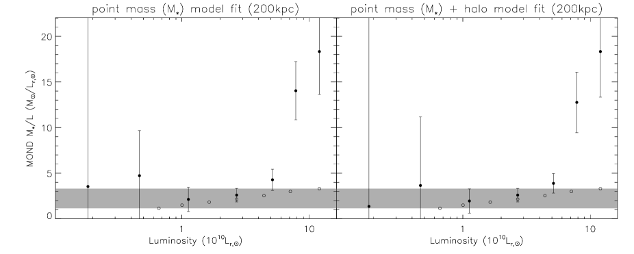
Figure 5: Left panel: the inferred MOND mass-to-light ratio as a function of luminosity. The derived MOND masses are obtained by fitting a point mass model to the SDSS lensing data within 200 kpc. Because there is no dark matter in MOND, we take the derived MOND mass to be the total stellar mass $M_{*}$ (we can ignore the contribution from HI). Right panel: The MOND mass-to-light ratio from a fit to the SDSS data when we add a neutrino halo to the stellar mass. The neutrino halo is assumed to have a $\beta$ profile and its total mass is three times of the stellar mass. The stellar mass-to-light ratios as a function of luminosity from Mandelbaum et al (2006) are indicated by the open circles. The shaded area indicates the range in those inferred stellar mass-to-light ratios.

4 results

Figure 3 shows the measurement of the Einstein radius as a function of the stellar mass of the lens. The left panel shows the results for the RCS data and the right panel corresponds to the results for the SDSS data. The Einstein radii in Fig. 3 have been scaled to $D_{ls}/D_{s}=1$. We assume a power-law relation between the Einstein radius and the stellar mass: $r_{E}\propto M_{*}^{\alpha}$. For reference, the dotted lines in Figure 3 show the best fit relation for $\alpha=0.5$, which is the expected slope for MOND.

Before we proceed with our determination of the scaling relation between lensing signal and stellar mass, we first examine whether the amplitudes of the signal agree between RCS and SDSS. For the comparison we adopt $\alpha=0.75$ and obtain a value of $r_{E}=0\hbox{$.\!\!^{\prime\prime}$}52\pm 0\hbox{$.\!\!^{\prime\prime}$}06$ for a galaxy with a stellar mass of $M_{*}=5\times 10^{10}M_{\odot}$ for the RCS measurements. For the SDSS data we obtain a value of $r_{E}=0\hbox{$.\!\!^{\prime\prime}$}42\pm 0\hbox{$.\!\!^{\prime\prime}$}03$, in fair agreement with the RCS results.

For the RCS data we find a best fit power-law slope of $\alpha=0.71\pm 0.15$ ($\chi_{\rm min}^{2}=4.5$ for 5 degrees of freedom; we marginalize over the normalization). The difference in $\chi^{2}$ $(\Delta\chi^{2}=\chi^{2}-\chi^{2}_{\rm min})$ as a function of $\alpha$ is indicated by the dotted line in Figure 4. For the SDSS data we find $\alpha=0.75\pm 0.09$ ($\chi_{\rm min}^{2}=4.9$ for 5 degrees of freedom) and the corresponding $\Delta\chi^{2}$ is indicated by the long-dashed curve in Figure 4. Combining the RCS and SDSS constraints yields a value $\alpha=0.74\pm 0.08$. (solid line in Figure 4). Hence we find good agreement between the RCS and SDSS data, with the SDSS data providing the best contraint. Furthermore, the inferred slope for the combined data is larger than $\alpha=0.5$ (which is the value predicted by MOND) with 99.7% confidence. Our results are also in good agreement with Conroy et al. (2007) who found that the velocity dispersion of satellite galaxies scales with the stellar mass of the host galaxy $\sigma\propto M_{*}^{0.4\pm 0.1}$, which corresponds to $r_{E}\propto M_{*}^{0.8}$ for an isothermal sphere model.

An alternative way to present our measurements is to consider the mass-to-light ratio as a function of luminosity. We expect the inferred MOND mass-to-light ratio to correspond to the stellar mass-to-light ratio, because in this case the stellar mass is the only source of gravity (we can ignore the contribution from neutral hydrogen). The left panel in Figure 5 shows the derived MOND mass-to-light ratio as a function of luminosity. The mass is determined from a fit to the SDSS lensing signal out to 200 kpc, assuming a point mass model for the galaxy.

Interestingly, at low luminosities the mass-to-light ratio is constant with values in agreement with what one might expect for an old population (the shaded region indicates the range of stellar M/L from Mandelbaum et al., 2006). At high luminosities, however, we observe a significant increase in $M/L$ which is inconsistent with the expected values for the stellar populations. Hence, these measurements suggest the need for additional (dark) matter.

4.1 Potential biases

The data points at high stellar mass in Figure 3 (and at high luminosity in Fig. 5 as well) carry much of the statistical weight, both for RCS and SDSS. It is apparent that if we were to remove or lower those measurements, the remaining data suggest a slope consistent with the MOND prediction, instead of the steeper relation determined in the previous section. Here we argue that those data points cannot be ignored, because they are in fact the more reliable measurements.

Compared to brighter galaxies, the lensing signal around a faint galaxy is more easily affected by the contribution of neighboring bright galaxies. Although we have selected ‘isolated’ or underdense lens samples for our analysis, the lensing signal in the low luminosity bins is potentially biased to higher values, thus lowering the inferred slope. In contrast, this will not be significant for the high luminosity bins, especially on small scales. To investigate this further we examined the effect of environment on the lensing signal around bright galaxies. The panels for L5b and L6f in Figure 3 from Mandelbaum et al (2006) correspond to our two highest luminosity bins. These results suggest there are no significant differences in the lensing signals on small scales ($\sim 200$ kpc) between the overdense and underdense samples. This implies that on these small scales the contribution of the environment to the lensing signals is negligible and the signal is dominated by the lens itself. Finally, the agreement between the RCS and SDSS results, which are based on different selection algorithms for the lenses, suggest the measurements are robust.

4.2 Neutrino Halos

The arguments presented in the previous section suggest the need for dark matter in luminous galaxies, even in the context of MOND. Similarly, MOND cannot explain observations of clusters of galaxies without invoking a significant dark matter component (Sanders, 2007): the MOND dynamical mass is about a factor $3-4$ times larger than the observed baryonic mass. Sanders (2007) suggests that active neutrinos with a mass $m_{\nu}\sim 2$eV might be able to reconcile these observations with MOND.

Neutrinos with masses in the range of a few eV cannot accumulate into dense halos around galaxies because of phase-space constraints (Tremaine & Gunn 1979). Nonetheless, as argued by Sanders (2007) galaxies may be able to acquire a neutrino halo, which would have a mass $\sim 1.4m_{\nu}$ times larger than the baryonic mass. This ratio of masses is set by the cosmological density of neutrinos and the baryon density inferred from CMB observations (Spergel et al., 2007). In this section we examine the effect of such a massive neutrino halo on the observed g-g lensing signal. Following Sanders (2007) we consider a mass of $m_{\nu}=2$eV. We note that this is the maximum mass allowed by $\beta$-decay experiments, which restrict the mass of the electron neutrino to a value less than 2eV (Yao et al., 2006).

We add a neutrino halo model to the stellar component (which we model by a point mass). A self-gravitating halo consisting of neutrinos (near the degeneracy limit) can be approximated by a $\gamma=5/3$ polytrope, which has a constant density core with a rapid decline beyond a core radius $R_{c}$ (Sanders, 2007). To simplify our calculations we approximate this polytrope by a $\beta$-model profile with $\beta=4/3$:

$$\rho(r)=\rho_{0}\left[1+\left(\frac{r}{R_{c}}\right)^{2}\right]^{-2},$$ (10)

where $\rho_{0}$ is the central density

$$\rho_{0}=\frac{3M_{\nu}}{\pi^{2}R_{c}^{3}}=\frac{3}{\pi^{2}R_{c}^{3}}\times 1.4m_{\nu}M_{*},$$ (11)

and the core radius $R_{c}$, which follows from the polytrope model, is given by (Sanders 2007)

$$R_{c}=1.8\left(\frac{m_{\nu}}{1eV}\right)^{-4/3}{(\frac{M_{\nu}}{10^{14}M_{\odot}}\frac{1}{0.06})}^{{1}\over{12}}{~{}\rm Mpc}.$$ (12)

We also explored a uniform density sphere with radius $R_{c}$, and found that the results are similar to the ones described below. The procedure used to compute the corresponding lensing signal in MOND is outlined in Appendix A. The (maximum) mass of the neutrino halo is set by the ratio of the cosmological baryon and neutrino densities, which for the adopted neutrino mass is approximately three times that of the stellar mass (e.g., Sanders, 2007). In doing so we assume that only the three known families of active neutrinos are relevant. A massive sterile neutrino cannot be ruled out by our analysis. However, invoking such a particle, which mimicks cold dark matter, would defeat the rationale behind developing an alternative theory of gravity.

Figure 6 shows the best fit model to the SDSS measurements for the highest luminosity bin. Note that the stellar mass is the only parameter in the fit. The best fit model, with a stellar mass of $(2.2\pm 0.6)\times 10^{12}M_{\odot}$, yields a core radius of $R_{c}=720$ kpc. Hence, the inferred mass-to-light ratio is $18.3\pm 4.7M/L_{r,\odot}$, much higher than what is expected from realistic stellar populations. Note that the model is fitted to the measurements within 200 kpc. Figure 6 shows that on these scales the stellar component dominates the lensing signal and that the neutrino halo only becomes relevant on large scales. This may seem surprising because the neutrino halo is much more massive than the stellar component. It is, however, important to recall that the weak lensing shear measures mass contrasts: for instance, a constant sheet of matter does not introduce a shear (Gorenstein et al. 1988). As a result, it is not the mass of the halo that is most relevant for our study, but the fact that the halo is very extended and has a large constant density core.

We verified that our results do not depend our choice of parameters. First of all, the results are robust against varying the value of $\beta$. This is not surprising because the size of the constant density core is the main relevant parameter. To examine possible (model) uncertainties in the calculation of the core radius, we also considered an extreme case with $R_{c}=360$ kpc. We find no qualitative difference: the core remains too large to produce a sufficiently large shear at small radii. Finally we note that adopting a different neutrino mass does not yield satisfactory results. A more massive neutrino results in a smaller core radius, but the resulting signal at large radii exceeds the lensing signal beyond 200kpc. We do not use those scales in our fits, because they may be biased high. They can, however, be considered upper limits and models that exceed the observed large scale values are therefore strongly disfavoured. A lower value for the neutrino mass results in an even larger core radius and lower lensing signal.

Figure 6: Fit to the SDSS data for the highest luminosity bin. A model consisting of a point mass of $M_{*}$ (stellar component) and a neutrino halo with a mass $3\times M_{*}$ is fitted to the measurements within 200 kpc. The compact stellar mass dominates the lensing signal on small scales and as a result, our results are insensitive to the effects of a neutrino halo.

Consequently, the inferred stellar mass-to-light ratio is reduced only slightly compared to our original results. This is clearly demonstrated in the right panel of Figure 5, which shows the resulting mass-to-light ratios. We therefore conclude that including a halo of active neutrinos around the lens galaxies cannot explain the high mass-to-light ratios. Similar conclusions have also been reached in studies of galaxy clusters (e.g., Takahashi & Chiba 2007; Natarajan & Zhao 2008). Finally we note that these findings suggest we can safely ignore the contribution from neutrinos in our study of the scaling relations.

A related issue arises from the fact that the most luminous galaxies are located in filaments. The filaments can in principle contribute a significant amount of mass along the line-of-sight, which was studied in Feix et al. (2007). In their model, the filament induces a shear which is uniform over scales much larger than the ones we study here. A constant shear will cancel when we compute the azimuthally averaged shear around the lenses, and we therefore argue that filaments do not affect our small scale g-g lensing signal.

Similar to massive clusters of galaxies, many elliptical galaxies are surrounded by hot, ionized gas. This gas is observed in X-ray observations (e.g., Humphrey et al., 2006) and we need to consider its impact on our results. Humphrey et al. (2006) used Chandra observations to study the ionized gas around NCG720, NGC4125 and NGC6482, which are three field ellipticals. Hence, these galaxies resemble the lenses studied in our analysis. In all three cases, the X-ray observations allow Humphrey et al. (2006) to study the relative distribution of the stars, gas and dark matter. From their Figure 6 it is clear that the gas is much more extended than the stellar mass. Furthermore, the amount of gas inferred from the data is less than the stellar mass within 200 kpc.

To study the effect of an extended gas distribution we considered a range of $\beta$ models where we varied to core radius from 1kpc to 30kpc. The mass within 200 kpc was fixed to the stellar mass (as suggested by the results in Humphrey et al., 2006). The smaller core radius of the hot gas distribution does boosts the shear on small scales compared to the neutrino halo, but can only reduce the MOND mass-to-light ratio values by $\sim 20\%$.

5 Conclusions

We study the amplitude of the weak gravitational lensing signal as a function of lens luminosity around a sample of relatively isolated galaxies. We demonstrate how such a study can be used to test Modified Newtonian Dynamics (Milgrom 1983a). Compared to previous work, our study is a test of MOND on relatively large scales, where the differences between MOND and $\Lambda$CDM are expected to be large. We show that MOND predicts a Tully-Fisher-like relation between the lensing signal (as quantified by the Einstein radius) and the stellar mass $M_{*}$.

Our analysis of data from RCS and SDSS shows that the amplitude of the lensing signal as a function of stellar mass is well described by a power law with a best fit slope of $\alpha=0.74\pm 0.08$. This result is inconsistent with $\alpha=0.5$, the predicted slope of MOND. Uncertainties in the stellar populations used to derive the stellar masses are expected to be small and should not alter our result.

As a related test, we determined the MOND mass-to-light ratio as a function of lens luminosity. Our results require dark matter to explain the amplitude of the lensing signal for the most luminous galaxies. We examined whether our findings can be reconciled with MOND by considering a massive halo of active neutrinos. Such a halo is found to be too extended to produce a significant change in the g-g lensing signal on scales less than 200 kpc. Similarly, hot ionized gas observed around elliptical galaxies (e.g., Humphrey et al. 2006) cannot explain our results in the context of MOND.

Although in this paper we focussed on MOND, we note that our findings are relevant for any alternative theory of gravity. Such theories should not just attempt to explain the Tully-Fisher relation (i.e., the scaling of rotation curves on small scales), but also need to explain our lensing measurements. In our opinion this is an important (and non-trivial) test to pass. Similarly, more exotic neutrino models have been proposed (e.g., Zhao 2008), which can also be tested through galaxy-galaxy lensing. Finally we note that much larger surveys, such as the Canada-France-Hawaii Telescope Legacy Survey (CFHTLS), will significantly improve the data in the coming years.

Appendix A MOND lensing signal

The development of a relativistic form of MOND, known as Tensor-Vector-Scalar gravity (TeVeS), by Bekenstein(2004) has opened the way to confront the theory to observations of gravitational lensing. Fortunately the steps to compute the lensing quantities in TeVeS the same as those in General Relativity, but with a modified gravitational potential (Zhao 2006). In this Appendix we outline the calculation of the lensing signal in the context of MOND for (spherically) symmetric cases.

The first step is the calculation of the gravitational potential. In highly symmetric systems (e.g., spherical halos), the TeVeS potential can be approximated by a MOND potential (just like GR can be approximated by Newtonian dynamics). The MOND gravitational potential $\phi$ is determined by the equation

$$\vec{\nabla}\cdot[\mu{(|\vec{\nabla}{\phi}|/a_{0})}\vec{\nabla}{\phi}]=4\pi G\rho,$$ (13)

where $\rho$ is the mass density and $a_{0}$ $\approx 10^{-8}$cms^-2 is the MOND characteristic acceleration. The function $\mu$ is required to satisfy $\mu(x\gg 1)\approx 1$, so that Newtonian dynamics is recovered in the limit of large accelerations and $\mu(x\ll 1)\approx x$.

Note that the Newtonian gravitational potential $\phi_{N}$ is determined by the Poisson equation $\nabla^{2}{\phi_{N}}=4\pi G\rho$ and that the Newtonian acceleration is given by $\vec{g}_{N}=-\vec{\nabla}{\phi_{N}}$. Similarly, the MOND acceleration is defined as $\vec{g}=-\vec{\nabla}{\phi}$. With these definitions, the Newtonian acceleration $g_{N}$ and MOND acceleration $g$ are related through a curl field (Bekenstein & Milgrom, 1984):

$$\mu{(g/a_{0})}\vec{g}=\vec{g}_{N}+\nabla\times\vec{h}.$$ (14)

In highly symmetric systems (i.e. those with spherical, planar, or cylindrical symmetry), the second curl term in Eq.(14) vanishes (Bekenstein & Milgrom, 1984) and we have the exact result

$$\mu{(g/a_{0})}\vec{g}=\vec{g}_{N}.$$ (15)

Thus, although equation (13) is non-linear and is generally difficult to solve, the MOND acceleration $\vec{g}$ can be readily obtained from the Newtonian acceleration $\vec{g}_{N}$ in symmetric cases. In this paper we consider spherically symmetric objects and we adopt $\mu(x)=x/sqrt(1+x^{2})$, where $x=g/a_{0}$. This yields an acceleration in the MOND regime of $g=\sqrt{a_{0}g_{N}}$.

The next step is the calculation of the lensing signal itself, following Zhao (2006). In MOND the steps are similar to the GR case, except that the real mass density $\rho$ is replaced by an effective density $\rho_{\rm eff}$ which is related to the MOND gravitational potential by the Poisson equation:

$$\rho_{\rm eff}=\nabla^{2}{\phi}/4\pi G.$$ (16)

We note that $\nabla^{2}{\phi}$ can be computed using Eqn.(15) and an explicit form of the $\mu$ function, because $\nabla^{2}{\phi}=\nabla\cdot(\nabla{\phi})=\nabla\cdot(-g)$. Hence, we can obtain the effective density $\rho_{\rm eff}$ through the known Newtonian acceleration $g_{N}$.

The next step is the calculation of the effective projected surface density $\Sigma_{\rm eff}$, which is obtained by integrating the effective density $\rho_{\rm eff}$ along the line of sight:

$$\Sigma_{\rm eff}(x,y)=\int_{-\infty}^{+\infty}\rho_{eff}(x,y,z)\,dz.$$ (17)

As discussed in §2, the convergence $\kappa$ in MOND is given by

$$\kappa(r)=\Sigma_{\rm eff}(r)/\Sigma_{\rm crit},$$ (18)

where the critical surface density is given by Eqn. (3). Finally, we compute the tangential shear using the relation between $\gamma_{T}$ and $\kappa$:

$$\gamma_{T}(r)={\bar{\kappa}(<r)}-\kappa(r),$$ (19)

where $\bar{\kappa}(<r)$ is the mean convergence within the radius $r$.

References

- (1) Adelman-McCarthy, J.K. et al. 2006, ApJS, 162, 38
- (2) Angus, G.W., H.Y., Zhao, H.S., Famaey, B., 2007, ApJ, 654, L13
- (3) Angus, G., Famaey, B., Tiret, O., Combes, F., Zhao, H.S., 2007 arXiv:0709.1966
- (4) Baumgardt H., Grebel E., Kroupa P., 2005, MNRAS, 359, L1
- (5) Bell, E.F., & de Jong, R.S. 2001, ApJ, 550, 212
- (6) Bekenstein, J. & Milgrom, M.: 1984, ApJ 286, 7
- (7) Bekenstein J., 2004, Phys. Rev. D, 70, 3509
- (8) Benjamin et al. 2007, MNRAS, 381, 702
- (9) Brainerd, T.G., Blandford, R.D., & Smail, I. 1996, ApJ, 466, 623
- (10) Chen, D.M. & Zhao H.S. 2006, ApJ, 650, L9
- (11) Chiu, M.-C., Ko, C.-M., Tian, Y. 2006, ApJ, 636, 565
- (12) Clowe, D., Bradac, M., Gonzalez, A.H., Markevitch, M., Randall, S.W., Jones, C. & Zaritski, D. 2006, ApJ, 648, L109
- (13) Corbelli, E., Salucci P., 2007, MNRAS, 374, 1051
- (14) Conroy. C, et al 2007 ApJ, 654, 153
- (15) Dodelson, S., & Liguori, M., 2006, Phys. Rev. Lett. 97, 231301
- (16) Famaey, B., & Binney, J., 2005, MNRAS, 363, 603
- (17) Ferreras, I., Saha, P., Williams, L.L.R., & Burles S. 2007, arXiv:0708.2151
- (18) Fischer, P., et al. 2000, AJ, 120, 1198
- (19) Gentile G., Famaey B., Combes F., Kroupa P., Zhao H. S., Tiret O., 2007, A&A, 472, L25
- (20) Gladders, M.D. & Yee, H.K.C. Yee 2005, ApJS, 157, 1
- (21) Gorenstein, M.V., Shapiro, I.I. & Falco, E.E. 1988, ApJ, 327, 693
- (22) Humphrey, P.J., Buote, D.A., Gastaldello, F., Zappacosta, L., Bullock, J.S., Brighenti, F., Mathews, W.G., 2006, ApJ, 646, 899
- (23) Hoekstra, H. & Jain, B. 2008, Ann. Rev. Nucl. and Part. Science, Volume 58, astro-ph/0805.0139
- (24) Hoekstra, H., Yee, H.K.C., Gladders, M.D., 2004, ApJ, 606, 67
- (25) Hoekstra, H., Hsieh, B.C., Yee, H.K.C., Lin, H., Gladders, M.D., 2005, ApJ, 635, 73 (H05)
- (26) Hsieh, B.C., Yee, H.K.C., Lin, H., & Gladders , M.D. 2005, ApJS, 158, 161
- (27) Klypin, A., Prada, F. 2007, preprint (arXiv:0706.3554)
- (28) Mandelbaum R., Seljak U., Kauffmann G., Hirata C. M., Brinkmann J., 2006, MNRAS, 368, 715 (M06)
- (29) McKay, T.A., et al. 2001, arXiv:astro-ph/0108013
- (30) McKay, T.A., et al., 2002, ApJ, 571, L85
- (31) Milgrom, M., 1983a, ApJ, 270, 365
- (32) Milgrom, M., 1983b, ApJ, 270, 371
- (33) Natarajan, P. & Zhao, H.S. 2008, MNRAS, in press, astro-ph/0806.3080
- (34) Navarro, J.F., Frenk, C.S., White, S.D.M., 1995, MNRAS, 275, 56
- (35) Nipoti, C., Londrillo, P., Zhao, H. S., Ciotti, L. 2007, MNRAS, 379, 597
- (36) Prada, F., et al. 2003, ApJ, 598
- (37) Parker, L.C., Hoekstra, H., Hudson, M.J., Van Waerbeke, L., Mellier, Y., et al., 2007, ApJ, 669, 21
- (38) Read, J.I., Moore, B., 2005, MNRAS, 361, 971
- (39) Sanders, R.H, McGaugh, S., 2002, ARA&A, 40, 263
- (40) Sanders, R.H., 2007, MNRAS, 380, 331
- (41) Seljak, U., 2000, MNRAS, 318, 203
- (42) Skordis C., Mota, D.F., Ferreira, P.G., Boehm, C., 2006, Phys. Rev. Lett., 96, 011301
- (43) Takahashi, R. & Chiba, T. 2007, ApJ, 671, 45
- (44) Tremaine, S.C. & Gunn, J.E. 1979, Phys. Rev. Lett., 42, 408
- (45) Spergel, D.N. et al. 2007, ApJS, 170, 377
- (46) Tully, R.B., Fisher, J.R., 1977, A&A, 54, 661
- (47) Feix, M., Xu, D., Shan, H.Y., Famaey, B., Limousin, M., Zhao, H.S., & Taylor, A. 2007, arXiv:0710.4935 (ApJ in press)
- (48) Yao, W.-M. et al. (Particle Data Group), 2006, J. Phys. G 33, 1 (URL:http://pdg.lbl.gov)
- (49) York, D.G. 2000, AJ, 120, 1579
- (50) Zaritsky, D., & White, S.D.M. 1994, ApJ, 435, 599
- (51) Zhao, H.S. 2005, A&A, 444, L25
- (52) Zhao, H.S., Bacon D., Taylor A.N., Horne K.D. 2006, MNRAS, 368, 171
- (53) Zhao, H.S., & Famaey, B. 2006, ApJ, 638, L9
- (54) Zhao, H.S. & Tian, L. 2006, A&A, 450, 1005
- (55) Zhao, H.S. 2006, astro-ph/0611777
- (56) Zhao, H.S. 2007, astro-ph/0704.0094
- (57) Zhao, H.S. 2008, arXiv:0805.4046
- (58) Zlosnik, T. G., Ferreira, P. G., Starkman, G. D., 2007, Phys. Rev. D, 75, 044017