Standard random walks and trapping on the Koch network
with scale-free behavior and small-world effect

Abstract

A vast variety of real-life networks display the ubiquitous presence of scale-free phenomenon and small-world effect, both of which play a significant role in the dynamical processes running on networks. Although various dynamical processes have been investigated in scale-free small-world networks, analytical research about random walks on such networks is much less. In this paper, we will study analytically the scaling of the mean first-passage time (MFPT) for random walks on scale-free small-world networks. To this end, we first map the classical Koch fractal to a network, called Koch network. According to this proposed mapping, we present an iterative algorithm for generating the Koch network, based on which we derive closed-form expressions for the relevant topological features, such as degree distribution, clustering coefficient, average path length, and degree correlations. The obtained solutions show that the Koch network exhibits scale-free behavior and small-world effect. Then, we investigate the standard random walks and trapping issue on the Koch network. Through the recurrence relations derived from the structure of the Koch network, we obtain the exact scaling for the MFPT. We show that in the infinite network order limit, the MFPT grows linearly with the number of all nodes in the network. The obtained analytical results are corroborated by direct extensive numerical calculations. In addition, we also determine the scaling efficiency exponents characterizing random walks on the Koch network.

I Introduction

Complex networks have been acknowledged as an invaluable tool for describing real-world systems in nature and society AlBa02 ; DoMe02 ; Ne03 ; BoLaMoChHw06 ; DoGoMe08 . Extensive empirical studies have uncovered that a lot of real networks share several remarkable features CoRoTrVi07 . One of the most relevant is the scale-free behavior, that is, various real networks exhibit a power-law degree distribution $P(k)\sim k^{-\gamma}$ BaAl99 . Another very important observation is that most real-life systems are characterized by ubiquitous small-world effect WaSt98 , including large clustering coefficient ZhZh07 and small average path length (APL) ZhZhChFaZhGu09 . Both the scale-free behavior and the small-world effect have a profound impact on almost all dynamical processes taking place on the networks Ne03 ; BoLaMoChHw06 ; DoGoMe08 ; AlJeBa00 ; CaNeStWa00 ; CoErAvHa00 ; CoErAvHa01 ; PaVe01a ; WaSt98 ; BaWe00 ; ZhZhZoCh08 .

Among various dynamical processes, random walks on networks are fundamental to many branches of science, and have received considerable attention from the scientific community NoRi04 ; SoRebe05 ; CoBeTeVoKl07 ; BeMeTeVo08 ; CoTeVoBeKl08 ; GaSoHaMa07 ; BaCaPa08 ; LeYoKi08 . As a primary dynamical process, random walks are related to a plethora of other dynamics such as transport in media HaBe87 , disease spreading LlMa01 , and target search JaBl01 ; Sh05 to name a few. On the other hand, random walks are useful for the study of topological structure (e.g. betweenness and average path length NoRi04 ; LeYoKi08 ) and community detection NeGi04 on networks. In particular, as an integral theme of random walks, trapping is related to a wide variety of contexts CaAb08 , such as photon-harvesting processes in photosynthetic cells Mo69 ; WhGo99 and characterizing similarities between the elements of a database FoPiReSa07 . It is thus of theoretical and practical interests to study standard random walks and trapping problem on complex networks.

The main interesting quantity closely related to random walks is the mean first-passage time (MFPT), and a central issue in the study of random walks is how the MFPT scales with the size of the system HaBe87 ; MeKl04 ; BuCa05 . In the past several years, a lot of endeavors have been devoted to studying the intrinsic relations between the scaling behavior of random walks and the underlying topological structure of networks NoRi04 ; SoRebe05 ; CaAb08 ; HuXuWuWa06 . The results of these investigations uncovered many unusual and exotic features of complex networks, especially of small-world and scale-free networks. In spite of their useful insight, most of previous jobs focused on numerical investigation, the analytical results of MFPT (in particular the average for all pairs of nodes) for standard random walks and trapping problem have been far less reported, with the exception of some graphs with simple topology, such as regular lattices Mo69 , Sierpinski fractals KaBa02PRE ; KaBa02IJBC , T fractal Ag08 , and deterministic scale-free trees Bobe05 ; ZhZhZhYiGu09 , as well as other structures CoBeTeVoKl07 ; BeMeTeVo08 ; CoTeVoBeKl08 , and exhaustive analytical research on scale-free and small-world networks with loops is still missing.

In this paper, we analytically investigate the scaling behavior of MFPT on complex networks with scale-free phenomenon and small-world effect. To achieve this goal, we first propose a relevant deterministic network, named Koch network, which is based on the classical fractal—Koch curve. We then suggest a minimal iterative algorithm generating the Koch network, on the basis of which we give in detail a scrutiny of the network architecture. The analysis results show that the Koch network is simultaneously scale free, small world, and has large clustering coefficient. Particularly, we show that the Koch network is completely two-point uncorrelated by exactly computing two relevant quantities of two-point correlations, which has never been previously found in other deterministically growing networks. Eventually, we study the scalings of MFPT on the proposed network for the standard random walks, together with a special case of trapping problem with the trap fixed at a hub node. We present that the MFPT averaged over all couples of nodes scales linearly with the network order (total number of nodes). We derive a closed-form solution for the MFPT characterizing the trapping process, which also grows as a linear function of the network order. We also compare the our results with those previously obtained for other scale-free networks.

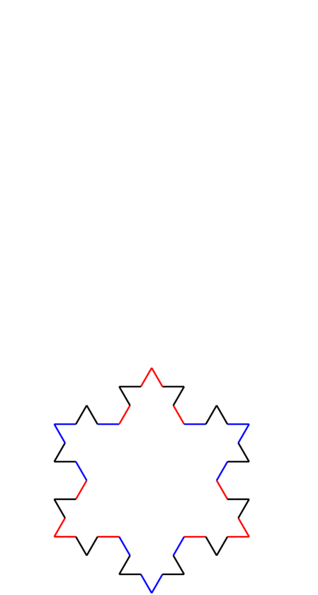
Figure 1: (Color online) The first two generations of the construction for Koch curve.

II Network construction

The network under consideration is derived from the Koch curve. To define the network, we first introduce the classical fractal, Koch island, also known as Koch curve, Koch snowflake or Koch triangle, which was proposed by Koch Ko1906 . This well-known fractal denoted by $S_{t}$ after $t$ generations is constructed as follows LaVaMeVa87 . Start with an equilateral triangle and denote this initial configuration as $S_{0}$. Perform a trisection of each side of this initial triangle and construct an equilateral triangle on each middle segment, so that the interior of the added triangle lies in the exterior of the base triangle, then remove the segment upon which the new triangle is established. Thus, we get $S_{1}$. For each line segment in $S_{1}$, trisect it and draw an equilateral triangle based on the resultant middle small segment to obtain $S_{2}$. Repeat recursively the procedure of trisection of existing line segments in last generation and addition of triangles. In the infinite $t$ limit, we obtain the famous Koch curve $S_{t}$, whose Hausdorff dimension is $d_{f}=\frac{2\ln 2}{\ln 3}$ Ma82 . In Fig. 1, we show schematically the structure of $S_{2}$. In fact, this fractal can be easily generalized to other dimensions LaVaMeVa87 .

From the Koch curve we can easily construct a network (called Koch network) using a simple mapping as follows. In the Koch network, nodes (vertices and sites) correspond to the sides (excluding those deleted) of the triangles constructed at all generations of the Koch curve as shown in Fig. 1. That is to say, for every triangle created at some generation, its two newly-born sides are mapped to two nodes, while the removed side is not. We make two nodes connected if the corresponding two sides of the Koch curves contact each other. For uniformity, the three sides of the initial equilateral triangle of $S_{0}$ also correspond to three different nodes. Note that after the birth of each side of a triangle constructed at a given generation, although some segments of it will be deleted at subsequent steps, we look upon its remaining segments as a whole and map it to only one node. Figure 2 shows the network associated with $S_{2}$.

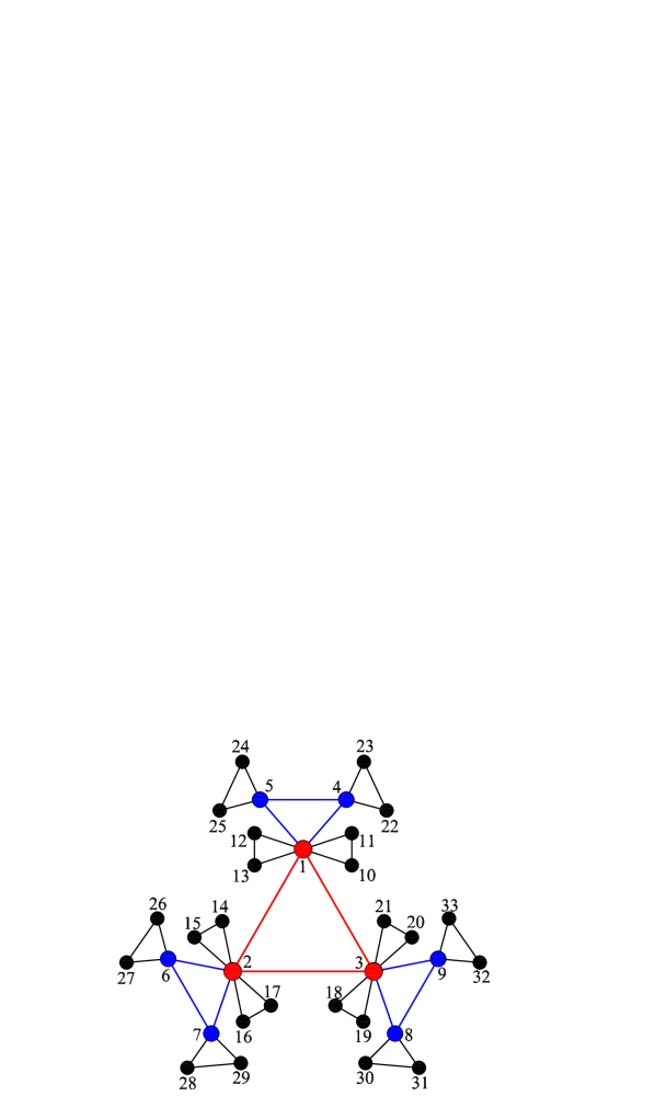
Figure 2: (Color online) Construction for the Koch network and labels of its nodes, showing the first two steps.

III Generation algorithm of Koch network

According to the construction process of Koch curve and the proposed mapping from Koch curve to Koch network, we can introduce with ease an iterative algorithm to create Koch network, denoted by $K(t)$ after $t$ generation evolutions. The algorithm is as follows. Initially ($t=0$), $K(0)$ consists of three nodes forming a triangle. Then, each of the three nodes of the initial triangle gives birth to two nodes. These two new nodes and its mother node are linked to each other shaping a new triangle. Thus we get $K(1)$ (see Fig. 3). For $t\geq 1$, $K(t)$ is obtained from $K(t-1)$. We replace each of the existing triangles of $K(t-1)$ with the connected cluster on the right-hand side (rhs) of Fig. 3 to obtain $K(t)$. The growing process is repeated until the network reaches a desired order. Figure 2 shows the network growth process for the first two steps.

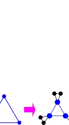
Figure 3: (Color online) Iterative construction method for the network.

Next we compute the order and the size (number of all edges) of Koch network $K(t)$. To this end, we first calculate the total number of triangles existing at step $t$, which we denote as $L_{\Delta}(t)$. By construction, this quantity increases by a factor of 4, i.e., $L_{\Delta}(t)=4\,L_{\Delta}(t-1)$. Considering the initial condition $L_{\Delta}(0)=1$, it follows that $L_{\Delta}(t)=4^{t}$. Let $L_{v}(t)$ and $L_{e}(t)$ be the respective number of nodes and edges created at step $t$. Notice that each triangle in $K(t-1)$ will lead to an addition of six new nodes and nine new edges at step $t$, then one can easily obtain the following relations: $L_{v}(t)=6\,L_{\Delta}(t-1)=6\times 4^{t-1}$ and $L_{e}(t)=9\,L_{\Delta}(t-1)=9\times 4^{t-1}$ for arbitrary $t>0$. From these results, we can compute the order and the size of Koch network. The total number of vertices $N_{t}$ and edges $E_{t}$ present at step $t$ is

$$N_{t}=\sum_{t_{i}=0}^{t}L_{v}(t_{i})=2\times 4^{t}+1$$ (1)

and

$$E_{t}=\sum_{t_{i}=0}^{t}L_{e}(t_{i})=3\times 4^{t},$$ (2)

respectively. Thus, the average degree is

$$\langle k\rangle=\frac{2E_{t}}{N_{t}}=\frac{6\times 4^{t}}{2\times 4^{t}+1},$$ (3)

which is approximately $3$ for large $t$, showing that Koch network is sparse as most real systems.

IV Structural properties of Koch network

Now we study some relevant characteristics of Koch network $K(t)$, focusing on degree distribution, clustering coefficient, average path length, and degree correlations.

IV.1 Degree distribution

We define $k_{i}(t)$ as the degree of a node $i$ at time $t$. When node $i$ is added to the network at step $t_{i}$ ($t_{i}\geq 0$), it has a degree of $2$, viz., $k_{i}(t_{i})=2$. To determine $k_{i}(t)$, we first determine the number of triangles involving node $i$ at step $t$ that is represented by $L_{\Delta}(i,t)$. These triangles will create new nodes connected to the node $i$ at step $t+1$. Then at step $t_{i}$, $L_{\Delta}(i,t_{i})=1$. By construction, $L_{\Delta}(i,t)=2\,L_{\Delta}(i,t-1)$. Since $L_{\Delta}(i,t_{i})=1$, one can derive $L_{\Delta}(i,t)=2^{t-t_{i}}$. Note that the relation between $k_{i}(t)$ and $L_{\Delta}(i,t)$ satisfies:

$$k_{i}(t)=2\,L_{\Delta}(i,t)=2^{t+1-t_{i}}.$$ (4)

In this way, at time $t$ the degree of node $i$ has been computed explicitly. From Eq. (4), one can see that at each step the degree of a node doubles, i.e.,

$$k_{i}(t)=2\,k_{i}(t-1).$$ (5)

Equation (4) shows that the degree spectrum of Koch network is discrete. It follows that the cumulative degree distribution Ne03 is given by

$$P_{\rm cum}(k)=\frac{1}{N_{t}}\,\sum_{\tau\leq t_{i}}L_{v}(\tau)={2\times 4^{t_{i}}+1\over 2\times 4^{t}+1}.$$ (6)

Substituting for $t_{i}$ in this expression using $t_{i}=t+1-\frac{\ln k}{\ln 2}$ gives

$$P_{\rm cum}(k)=\frac{2\times 4^{t}\times 4\times k^{-(\ln 4/\ln 2)}+1}{2\times 4^{t}+1}.$$ (7)

When $t$ is large enough, one can obtain

$$P_{\rm cum}(k)=4\times k^{-2}.$$ (8)

So the degree distribution follows a power-law form with the exponent $\gamma=3$. Note that this exponent of degree distribution is the same as that of the Barabási-Albert (BA) model BaAl99 .

Before closing this section, we compute another quantity $\langle k^{2}\rangle$, i.e., the fluctuations of the connectivity distribution, which is useful for the calculation of Pearson correlation coefficient that will be discussed in the following text. The quantity $\langle k^{2}\rangle$ is given by

$$\langle k^{2}\rangle=\frac{1}{N_{t}}\sum_{t_{i}=0}^{t}L_{v}(t_{i})\left[k(t_{i},t)\right]^{2},$$ (9)

where $k(t_{i},t)$ is the degree of a node at step $t$ which was generated at step $t_{i}$. Combining previously obtained results, we find

$$\langle k^{2}\rangle=\frac{2\times 4^{t}(3t+6)}{2\times 4^{t}+1}.$$ (10)

IV.2 Clustering coefficient

The clustering coefficient WaSt98 of a node $i$ with a degree $k_{i}$ is given by $C_{i}=2e_{i}/[k_{i}(k_{i}-1)]$, where $e_{i}$ is the number of existing triangles attached to node $i$, and $k_{i}(k_{i}-1)/2$ is the total number of possible triangles including $i$. Using the connection rules, it is straightforward to calculate analytically the clustering coefficient $C(k)$ for a single node with degree $k$. In the preceding section, we have obtained $2\,e_{i}=k_{i}$ for all nodes at all steps. So there is a one-to-one correspondence between the clustering coefficient of a node and its degree. For a node of degree $k$, we have

$$C(k)=\frac{1}{k-1},$$ (11)

which is inversely proportional to $k$ in the limit of large $k$. The scaling of $C(k)\sim k^{-1}$ has been observed in many real-world scale-free networks RaBa03 .

After $t$ generation evolutions, the clustering coefficient $C_{t}$ of the whole network, defined as the average of $C_{i}\,^{{}^{\prime}}s$ over all nodes in the network, is given by

$$C_{t}=\frac{1}{N_{t}}\sum_{r=0}^{t}\left[\frac{1}{M_{r}-1}L_{v}(r)\right],$$ (12)

where the sum runs over all the nodes and $M_{r}$ is the degree of those nodes created at step $r$, which is given by Eq. (4). In the limit of large $N_{t}$, Eq. (12) converges to a nonzero value $C=0.82008$, as shown in Fig. 4. Therefore, the Koch network is highly clustered.

Figure 4: Semilogarithmic plot of average clustering coefficient $C_{t}$ versus network order $N_{t}$.

IV.3 Average path length

Let $d_{t}$ denote the APL of the Koch network $K(t)$. Since the Koch network is self-similar, the APL can be computed analytically to obtain an explicit formula, by using a method similar to but different from those in Refs. HiBe06 ; ZhChZhFaGuZo08 . We represent all the shortest path lengths of $K(t)$ as a matrix in which the entry $d_{ij}$ is the shortest distance from node $i$ to node $j$, then $d_{t}$ is defined as the mean of $d_{ij}$ over all couples of nodes,

$$d_{t}=\frac{D_{t}}{N_{t}(N_{t}-1)/2}\,,$$ (13)

where

$$D_{t}=\sum_{\stackrel{{\scriptstyle i\in K(t),\,j\in K(t)}}{{i\neq j}}}d_{ij}$$ (14)

denotes the sum of the shortest path length between two nodes over all pairs. It should be mentioned that in Eq. (14), for a couple of nodes $i$ and $j$ ($i\neq j$), we only count $d_{ij}$ or $d_{ji}$, not both. In the Appendix, we provide the detailed derivation for the APL. The obtained analytical expression for $d_{t}$ is

$$d_{t}=\frac{4+14\times 4^{t}+12t\times 4^{t}}{3\,(4^{t}+1)},$$ (15)

which approximates $4t$ in the infinite $t$, implying that the APL shows a logarithmic scaling with the network order. Therefore, the Koch network exhibits a small-world behavior. We have checked our analytical result against numerical calculations for different network orders up to $t=10$ which corresponds to $N_{10}=1\,048\,577$. In all the cases we obtain a complete agreement between our theoretical formula and the results of numerical investigation (see Fig. 5).

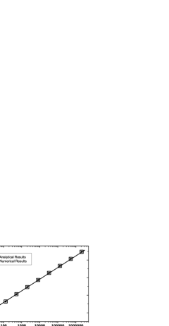
Figure 5: Average path length $d_{t}$ versus network order $N_{t}$ on a semilogarithmic scale. The solid line is a guide to the eye.

IV.4 Degree correlations

Degree correlations are a particularly interesting subject in the field of network science MsSn02 , because they can give rise to some interesting network structure effects. An interesting quantity related to degree correlations is the average degree of the nearest neighbors for nodes with degree $k$, denoted as $k_{\rm nn}(k)$, which is a function of node degree $k$ PaVaVe01 . When $k_{\rm nn}(k)$ increases with $k$, it means that nodes have a tendency to connect to nodes with a similar or larger degree. In this case the network is defined as assortative Newman02 . In contrast, if $k_{\rm nn}(k)$ is decreasing with $k$, which implies that nodes of large degree are likely to have near neighbors with small degree, then the network is said to be disassortative. If correlations are absent, $k_{\rm nn}(k)={\rm const}$.

We can exactly calculate $k_{\rm nn}(k)$ for Koch network using Eqs. (4) and (5) to work out how many links are made at a particular step to nodes with a particular degree. By construction, we have the following expression DoMa05 ; ZhZhZoChGu07 :

$$k_{\rm nn}(k) = {1\over L_{v}(t_{i})k(t_{i},t)}\Bigg{(}\sum_{t^{\prime}_{i}=0}^{t^{\prime}_{i}=t_{i}-1}L_{v}(t^{\prime}_{i})k(t^{\prime}_{i},t_{i}-1)k(t^{\prime}_{i},t)$$ (16)

$$+\sum_{t^{\prime}_{i}=t_{i}+1}^{t^{\prime}_{i}=t}L_{v}(t_{i})k(t_{i},t^{\prime}_{i}-1)k(t^{\prime}_{i},t)\Bigg{)}+1$$

for $k=2^{t+1-t_{i}}$. Here the first sum on the right-hand side accounts for the links made to nodes with larger degree (i.e., $t^{\prime}_{i}<t_{i}$) when the node was generated at $t_{i}$. The second sum describes the links made to the current smallest degree nodes at each step $t^{\prime}_{i}>t_{i}$. The last term 1 accounts for the link connected to the simultaneously emerging node. After some algebraic manipulations, we obtain exactly

$$k_{\rm nn}(k)=t+2.$$ (17)

Therefore, two node correlations do not depend on the degree. On the other hand, Eq. (17) shows that for large $t$, $k_{\rm nn}(k)$ is approximately a logarithmic function of the network order $N_{t}$, namely $k_{\rm nn}(k)\sim\ln N_{t}$. Note that the same behavior has also been observed in the BA model VapaVe02 .

Degree correlations can be also described by a Pearson correlation coefficient $r$ of degrees at either end of a link. It is defined as Newman02 ; DoMa05 ; RaDoPa04

$$r={\langle k\rangle\langle k^{2}k_{\rm nn}(k)\rangle-\langle k^{2}\rangle^{2}\over\langle k\rangle\langle k^{3}\rangle-\langle k^{2}\rangle^{2}}.$$ (18)

If the network is uncorrelated, the correlation coefficient equals zero. Disassortative networks have $r<0$, while assortative graphs have a value of $r>0$. Substituting Eqs. (3), (10), and (17) into Eq. (18), we can easily see that for arbitrary $t\geq 0$, the numerator of Eq. (18) is always equal to zero. Thereby, $r$ also equals zero, which again indicates that Koch network shows the absence of degree correlations.

V Random walks

As addressed in Sec. IV, the Koch network exhibits exclusive topological properties not simultaneously shared by other networks. Thus, it is worthwhile to study dynamical processes occurring on the network. In this section we consider simple random walks on the Koch network defined by a walker such that at each step the walker, located on a given node, moves to any of its nearest neighbors with equal probabilities.

V.1 Scaling efficiency

We follow the concept of scaling efficiency introduced in Bobe05 . Denote by $T_{ij}$ the first-passage time (FPT) between two nodes $i$ and $j$ in a network. Let $T_{ii}$ be the mean time for a walker returning to a node $i$ for the first time after the walker has left it. When the network order grows from $N$ to $gN$, one expects that in the infinite limit of $N$

$$T_{ij}(gN)\sim g^{\delta_{ij}}T_{ij}(N),$$ (19)

where $\delta_{ij}$ is defined as the scaling efficiency exponent. An analogous relation for $T_{ii}$ defines an exponent $\delta_{ii}$.

One can confine the scaling efficiency in the nodes already existing in the network before growth. Let $T^{\prime}_{ij}(gN)$ be the mean first-passage time in the network under consideration, averaged over the original class of nodes (before growth). Then the restricted scaling efficiency exponent $\lambda_{ij}$ is defined by the relation

$$T^{\prime}_{ij}(gN)\sim g^{\lambda_{ij}}T_{ij}(N).$$ (20)

Similarly, we can define $\lambda_{ii}$.

After introducing the concepts, in the following we will investigate random walks on the Koch network following a similar but obviously different method used in Bobe05 ; ZhZhZhYiGu09 .

V.2 First-passage time for old nodes

Consider an arbitrary node $i$ in the Koch network $K(t)$ after $t$ generation evolution. Note that for the sake of simplicity, we also denote $K(t)$ by $K_{t}$, and both denotations will be used alternatively in the following text. From Eq. (5), we know that upon growth of the network to generation $t+1$, the degree $k_{i}$ of node $i$ doubles, that is to say, it increases from $k_{i}$ to $2k_{i}$. Let the FPT for going from node $i$ to any of the $k_{i}$ old neighbors be $T$ and let the FPT for going from any of the $k_{i}$ new neighbors to one of the $k_{i}$ old neighbors be $A$. Then we can establish the following equations (see Fig. 6):

$$\left\{\begin{array}[]{ccc}T&=&\frac{1}{2}+\frac{1}{2}(1+A),\\ A&=&\frac{1}{2}(1+T)+\frac{1}{2}(1+A),\end{array}\right.$$ (23)

which leads to $T=4$. Therefore, the passage time from any node $i$ ($i\in K_{t}$) to any node $j$ ($j\in K_{t+1}$) increases four times, on average, upon growth of the network to generation $t+1$, i.e.,

$$T^{\prime}_{ij}(N_{t+1})=4\,T_{ij}(N_{t}).$$ (24)

For explanation, see Refs. Bobe05 ; HaBe87 and related references therein. Since the network order approximately grows by four times in the large $t$ limit [see Eq. (1)]. This indicates that the scaling efficiency exponent for old nodes is $\lambda_{ij}=1$, which is the same as that of the recursive scale-free tree addressed in Ref. Bobe05 .

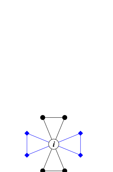
Figure 6: (Color online) Growth of trapping time in going from $K_{t}$ to $K_{t+1}$. Node $i\in K_{t}$ has $k_{i}$ neighbor nodes in generation $t$ ($\bullet$) and $k_{i}$ new neighbor nodes in generation $t+1$ ($\blacksquare$). A new neighbor of node $i$ has a degree of 2, and is simultaneously linked to another new neighbor of $i$.

Next we continue to consider the return of FPT to node $i$. Denote by $T^{\prime}_{ii}$ the FPT for returning to node $i$ in $K_{t+1}$. Denote by $T^{\prime}_{ji}$ the FPT from $j$—an old neighbor of $i$ ($i\in K_{t}$)—to $i$, in $K_{t+1}$. Analogously, denote by $T_{ii}$ the FPT for returning to $i$ in $K_{t}$ and denote by $T_{ji}$ the FPT from the same neighbor $j$, to $i$, in $K_{t}$. For $K_{t}$, we have

$$T_{ii}=\frac{1}{k_{i}}\sum_{j\in\Omega_{i}(t)}(1+T_{ji}),$$ (25)

where $\Omega_{i}(t)$ is the set of neighbors of node $i$, which belongs to $K_{t}$. On the other hand, for $K_{t+1}$,

$$T^{\prime}_{ii}=\frac{1}{2}\times 3+\left(1-\frac{1}{2}\right)\frac{1}{k_{i}}\sum_{j\in\Omega_{i}(t)}(1+T^{\prime}_{ji}).$$ (26)

The first term on the rhs of Eq. (26) accounts for the process in which the walker moves from node $i$ to its new neighbors and back. Since among all neighbors of node $i$, half of them are new, which is obvious from Eq. (5), such a process occurs with a probability of $\frac{1}{2}$ and takes three time steps. The second term on the rhs interprets the process where the walker steps from $i$ to one of the old neighbors $j$ previously existing in $K_{t}$ and back; this process happens with the complimentary probability $(1-\frac{1}{2})$.

Using Eq. (24) to simplify Eq. (26), we can obtain

$$T^{\prime}_{ii}=2\,T_{ii}=4^{1/2}\,T_{ii}.$$ (27)

In other words,

$$T^{\prime}_{ii}(N_{t+1})=4^{1/2}\,T_{ii}(N_{t}).$$ (28)

Thus, the scaling efficiency exponent $\lambda_{ii}=\frac{1}{2}$, which is less than 1. Recall that for the recursive scale-free tree, its scaling efficiency exponent is $\lambda_{ii}=1-\frac{\ln 2}{\ln 3}<\frac{1}{2}$ Bobe05 , which means that in the Koch network it is more difficult for the walker to return to the origin than in the recursive scale-free tree, when the networks grow in size.

V.3 First-passage time for all nodes

We continue to compute $T_{j^{\prime}j^{\prime}}$, which is the FPT to return to a new node $j^{\prime}\in K_{t}$ that is a neighbor of node $i\in K_{t-1}$. Notice that when $j^{\prime}$ was generated, another node $j^{\prime\prime}$ emerged simultaneously, connected to $i$ and $j^{\prime}$ (see Fig. 6). Denote by $T_{1}$ the FPT from $i$ to $j^{\prime}$ and denote by $B$ the FPT to return to $i$ (starting off from $i$) without ever visiting $j^{\prime}$ and $j^{\prime\prime}$. Then we have

$$T_{j^{\prime}j^{\prime}}=\frac{1}{2}(1+T_{1})+\frac{1}{2}(1+T_{j^{\prime\prime}j^{\prime}}),$$ (29)

$$T_{j^{\prime\prime}j^{\prime}}=\frac{1}{2}\times 1+\frac{1}{2}(1+T_{1}),$$ (30)

and

$$T_{1}=\frac{1}{k_{i}}+\frac{1}{k_{i}}(1+T_{j^{\prime\prime}j^{\prime}})+\frac{k_{i}-2}{k_{i}}(B+T_{1}).$$ (31)

Equation (31) can be interpreted as follows: with probability $\frac{1}{k_{i}}$ ($k_{i}$ being the degree of node $i$ in $K_{t}$), the walker starting from node $i$ would take one time step to go to node $j^{\prime}$; with probability $\frac{1}{k_{i}}$, the walker takes one time step to move to node $j^{\prime\prime}$ then takes time $T_{j^{\prime\prime}j^{\prime}}$ to reach $j^{\prime}$; and with the remaining probability $\frac{k_{i}-2}{k_{i}}$, the walker chooses uniformly a neighbor node except $j^{\prime}$ and $j^{\prime\prime}$ and spends on average time $B$ in returning to $i$ then takes time $T_{1}$ to arrive at node $j^{\prime}$.

In order to close Eqs. (29) and (31), we express the FPT to return to $i$ as

$$T_{ii}(N_{t})=\frac{1}{k_{i}}\times 3+\frac{1}{k_{i}}\times 3+\frac{k_{i}-2}{k_{i}}B.$$ (32)

Eliminating $T_{1}$, $T_{j^{\prime\prime}j^{\prime}}$, and $B$, we obtain

$$T_{j^{\prime}j^{\prime}}(N_{t})=\frac{k_{i}}{2}\,T_{ii}(N_{t}).$$ (33)

Combining Eqs. (4), (27), and (33), we have

$$T_{j^{\prime}j^{\prime}}(N_{t})=3\times 4^{t}\sim 3\,N_{t}.$$ (34)

Thus, in spite of the fact that simultaneously emerging new nodes are linked to different nodes with various degrees, they have the same mean return time. Iterating Eqs. (27) and (33), we have that in $K_{t}$ there are $L_{v}(\epsilon)$ ($0\leq\epsilon\leq t$) nodes with $T_{ii}=2^{t+1+\epsilon}$. This, together with Eqs. (2) and (4), means that for an arbitrary node $i$ (born at step $t_{i}$) with degree $k_{i}(t)=2^{t+1-t_{i}}$ at time $t$, the FPT to return to $i$ is $T_{ii}=\frac{2\,E_{t}}{k_{i}(t)}$. Note that a similar expression has been obtained for the periodic lattices Hu95 and random networks NoRi04 by using a different derivation method. Thus, the mean return time $T_{ii}$ is not reliant on the details of the global structure of Koch network. It only relies on the network size and the connectivity of the node: the larger the degree of the node, the smaller the FPT to return.

Taking the average of $T_{ii}$ over all nodes in $K_{t}$ leads to

$$\langle T_{ii}\rangle_{t} = \frac{1}{2\times 4^{t}+1}\big{(}3\times 2^{t+1}+6\times 2^{t+2}+6\times 4\times 2^{t+2}$$ (35)

$$\quad\quad\quad\quad\quad\quad\quad+6\times 4^{t-1}\times 2^{t+1+t}\big{)}$$

$$= \frac{1}{2\times 4^{t}+1}\left(\frac{24}{7}\times 16^{t}+\frac{18}{7}\times 2^{t}\right).$$

For infinite $t$, $\langle T_{ii}\rangle_{t}\approx\frac{12}{7}\times 4^{t}\sim N_{t}$, implying that $\delta_{ii}=1$, an efficiency scaling identical to that of the recursive scale-free tree Bobe05 . Therefore, the scalings of new nodes play a dominant role in the average of mean return time for all nodes.

Next we calculate $T_{ij}$ in $K_{t}$, which is FPT from an arbitrary node $i$ to another node $j$. Since each newly created node has a degree of 2 and is linked to an old node and a simultaneously emerging new node, and these three nodes form a triangle, the FPT $T_{i^{\prime}j}$ from node $i^{\prime}$—a new neighbor of the old node $i$—to $j$ equals $T_{ij}$ plus 2 (i.e., $T_{i^{\prime}i}$) and thus has little effect on the scaling when the network order $N$ is very large. Therefore, we need only to consider FPT $T_{ij^{\prime}}$ from $i$ to $j^{\prime}$—a new neighbor of $j$, which can be expressed as

$$T_{ij^{\prime}}=T_{ij}+T_{jj^{\prime}}.$$ (36)

Suppose that when $j^{\prime}$ was born, it connected to node $j$ and a simultaneously emerging node $j^{\prime\prime}$ (by construction, $j^{\prime\prime}$ was also linked to node $j$), then we have

$$T_{j^{\prime}j^{\prime}}=\frac{1}{2}(1+T_{jj^{\prime}})+\frac{1}{2}(1+T_{j^{\prime\prime}j^{\prime}}),$$ (37)

and

$$T_{j^{\prime\prime}j^{\prime}}=\frac{1}{2}+\frac{1}{2}(1+T_{jj^{\prime}}).$$ (38)

Inserting Eq. (38) to Eq. (37), we obtain

$$T_{jj^{\prime}}=\frac{4}{3}\,T_{j^{\prime}j^{\prime}}-2.$$ (39)

Substituting Eq. (39) and Eq. (34) for $T_{j^{\prime}j^{\prime}}$ into Eq. (36) results in

$$T_{ij^{\prime}}=T_{ij}+\frac{4}{3}\,T_{j^{\prime}j^{\prime}}-2\sim N_{t},$$ (40)

where Eq. (24) has been used. Therefore, we have

$$\langle T_{ij}\rangle_{t}\sim N_{t},$$ (41)

which shows that the mean transit time between arbitrary pairs of nodes is proportional to the network order. Equation (41) also reveals that $\delta_{ij}$ is a constant 1. Notice that the linear scaling of the average traverse time with network order has been previously obtained by numerical simulations for the Apollonian networks HuXuWuWa06 and the pseudofractal scale-free web Bobe05 , both of which have been well studied AnHeAnSi05 ; DoMa05 ; ZhCoFeRo06 ; ZhRoZh06 ; ZhGuXiQiZh09 ; KaHiBe09 ; DoGoMe02 ; CoFeRa04 ; ZhZhCh07 ; ZhRoZh07 ; RoHaAv07 ; ZhQiZhXiGu09 .

VI Random walk with a trap

In the preceding section, we have obtained the scaling between the MFPT and the network order. Although scaling theory is central in studying diffusive process on a variety of deterministic media, it has been noted that scaling laws do not provide a complete picture of dynamic phenomena on deterministic media, e.g., regular fractals Gi96 , and exact relationships are useful. In this section we study the trapping problem of a simple unbiased Markovian random walk of a particle on network $K_{t}$ in the presence of a trap or a perfect absorber located on a given node, which absorbs all particles visiting it. Our aim is to give some further insight into the trapping process and the independence of the average trapping time (TT) on the size of the underlying system, by providing a rigorous solution of the mean trapping time (MTT) as a function of the network order.

VI.1 Formulating the trapping problem

For the convenience of description, we distinguish different nodes by labeling all the nodes belonging to $K_{t}$ in the following way. The initial three nodes in $K_{0}$ are labeled as 1, 2, and 3, respectively. In each new generation, only the new nodes created at this generation are labeled, while the labels of all old nodes remain unchanged, i.e., we label new nodes as $M+1$, $M+2$, $\ldots$, $M+\Delta M$, where $M$ is the total number of the pre-existing nodes and $\Delta M$ is the number of newly created nodes. Eventually, every node is labeled by a unique integer, at time $t$ all nodes are labeled from 1 to $N_{t}=2\times 4^{t}+1$ (see Fig. 2).

Before proceeding further, we give the following definitions. Let $A_{ij}$ be an element of the adjacency matrix $\textbf{A}_{t}$ of network $K_{t}$ such that $A_{ij}=1$ if nodes $i$ and $j$ are connected by an edge and $A_{ij}=0$ otherwise. Thus, the degree of a vertex $i$ in $K_{t}$ is $d_{v_{i}}=\sum_{j}A_{ij}$. And the diagonal degree matrix $\textbf{D}_{t}$ of $K_{t}$ is defined by $\textbf{D}_{t}=\text{diag}(d_{v_{1}},d_{v_{2}},\ldots,d_{v_{i}},\ldots,d_{v_{N_{t}}})$. Finally, we define $\textbf{W}_{t}=\textbf{A}_{t}\cdot\textbf{D}_{t}^{-1}$, where $\textbf{D}_{t}^{-1}$ is the inverse matrix of $\textbf{D}_{t}$, then the normalized Laplacian matrix of network $K_{t}$ is $\textbf{L}_{t}=\textbf{I}_{t}-\textbf{W}_{t}$, in which $\textbf{I}_{t}$ is an identity matrix with order $N_{t}\times N_{t}$.

We locate the trap at node 1 (due to the symmetry, the trap can be also located at node 2 or 3, which does not have any effect on MFPT), denoted as $i_{T}$. Note that the particular selection we made for the trap location makes the analytical computation process (that will be shown in detail in the following text) easily iterated as we can identify the trap node $i_{T}$ since the first generation. At each time step (taken to be unity), the walker selects uniformly among the neighbors of the current node (excluding the trap) and takes a step to one of them. Since node 1 is one of the three nodes with the largest degree, it is easily seen that in the presence of the trap $i_{T}$ fixed on node 1, the walker will be inevitably absorbed Bobe05 .

This trapping process can be described by specifying the set of transition probabilities $W_{ij}$ for the particle of going from node $i$ (except the trap $i_{T}$) to node $j$. We can regard $W_{ij}$ as an element of the matrix $\textbf{W}_{t}^{T}$, which is a submatrix of $\textbf{W}_{t}$ with the row and the column corresponding to trap being removed. That is to say, $\textbf{W}_{t}^{T}$ is a $(N_{t}-1)$-order submatrix of $\textbf{W}_{t}$ with the first row and column being deleted. Similarly, one can define $\textbf{A}_{t}^{T}$, $\textbf{D}_{t}^{T}$, $\textbf{I}_{t}^{T}$ and $\textbf{L}_{t}^{T}$, thus we have $\textbf{W}_{t}^{T}=\textbf{A}_{t}^{T}\cdot(\textbf{D}_{t}^{T})^{-1}$ and $\textbf{L}_{t}^{T}=\textbf{I}_{t}^{T}-\textbf{W}_{t}^{T}$. The inverse of $\textbf{L}_{t}^{T}$, $(\textbf{L}_{t}^{T})^{-1}$, is the fundamental matrix of the Markovian chain representing the unbiased random walk with a trap.

An interesting quantity related to the trapping process is the mean residence time (MRT), which is the mean time that a random walker spends at a given site prior to being trapped. In fact, the MRT is the mean number of visitations of a given site by the walker before trapping occurs, and finding the MRT at node $i$, starting from node $j$, is equivalent to finding the element $L_{i,j}^{-1}$ of the fundamental matrix KeSn76 .

Another quantity of interest is the TT. In network $K_{t}$, the trapping time $T_{i}^{t}$ of a given site $i$ is the expected time for a walker starting from $i$ to first reach the trap. By definition, trapping time $T_{i}^{t}$ is the sum of the MRTs over all nodes except $i_{T}$, i.e.,

$$T_{i}^{t}=\sum_{j=2}^{N_{t}}{L_{ij}^{-1}}.$$ (42)

Then, the MTT or the mean first-passage time (MFPT), $\langle T\rangle_{t}$, which is the average of $T_{i}^{t}$ over all initial nodes distributed uniformly over nodes in $K_{t}$ other than the trap, is given by

$$\langle T\rangle_{t}=\frac{1}{N_{t}-1}\sum_{i=2}^{N_{t}}T_{i}^{t}=\frac{1}{N_{t}-1}\sum_{i=2}^{N_{t}}\sum_{j=2}^{N_{t}}{L_{ij}^{-1}}.$$ (43)

The quantities of TT and MTT are very important since they measure the efficiency of the trapping process: the smaller the two quantities, the higher the efficiency, and vice versa. Equations (42) and (43) show that the problem of calculating $T_{i}^{t}$ and $\langle T\rangle_{t}$ is reduced to finding the sum of elements of matrix $(\textbf{L}_{t}^{T})^{-1}$. In Tables 1 and 2, we list separately $T_{i}^{t}$ of some nodes and $\langle T\rangle_{t}$ for different network orders up to $t=6$. From Table 1, one can easily observe that for a given node $i$, the relation $T_{i}^{t+1}=4\,T_{i}^{t}$ holds. That is to say, upon growth of Koch network from $t$ generation to generation $t+1$, the trapping time to first reach the trap increases by a factor of 4, which is consistent with Eq. (24). This scaling relation is a basic character of the trapping process on the Koch network, which will be useful for deriving the formula of MTT that will be given in the following section.

Table 1: Trapping time $T_{i}^{t}$ for a random walker starting from node $i$ on $K_{t}$ for various $t$. Notice that owing to the obvious symmetry, nodes in a parentheses are equivalent, since they have the same trapping time. All the values are calculated straightforwardly from Eq. (42).

$t\backslash i$	$(2,3)$	$(4,5)$	$(6,7,8,9)$	$(10,11,12,13)$	$(14,15,16,17,18,19,20)$	$(22,23,24,25)$	$(26,27,28,29,30,31,32,33)$
0	$2$
1	$8$	$2$	$10$
2	$32$	$8$	$40$	$2$	$34$	$10$	$42$
3	$128$	$32$	$160$	$8$	$136$	$40$	$168$
4	$512$	$128$	$640$	$32$	$544$	$160$	$672$
5	$2048$	$512$	$2560$	$128$	$2176$	$640$	$2688$
6	$8192$	$2048$	$10240$	$512$	$8704$	$2560$	$10752$

Notice that the order of matrix $(\textbf{L}_{t}^{T})^{-1}$ is $(N_{t}-1)\times(N_{t}-1)$, where $N_{t}$ increases exponentially with $t$, as shown in Eq. (1). Thus, for large $t$, the computation of the TT and the MTT from Eqs. (42) and (43) is prohibitively time and memory consuming, making it difficult to obtain $T_{i}^{t}$ and $\langle T\rangle_{t}$ through direct calculation for large network; one can compute directly the MFPT only for the first several generations. However, the recursive construction of Koch network allows one to compute analytically the MTT to achieve a closed-form solution; the derivation details of which will be given in next section.

Table 2: Mean trapping time obtained by direct calculation from Eq. (43).

$t$	$N_{t}$	$\sum_{i=2}^{N_{t}}T_{i}^{t}$	$\langle T\rangle_{t}$
0	$3$	$4$	$4/2$
1	$9$	$60$	$60/8$
2	$33$	$896$	$896/32$
3	$129$	$13888$	$13888/128$
4	$513$	$219648$	$219648/512$
5	$2049$	$3501056$	$3501056/2048$
6	$8193$	$55951360$	$55951360/8192$

VI.2 Analytical solution for mean trapping time

We now determine the average of the mean time to absorption, aiming to derive an exact solution. We represent the set of nodes in $K_{t}$ as $\Lambda_{t}$ and denote the set of nodes created at generation $t$ by $\overline{\Lambda}_{t}$. Thus we have $\Lambda_{t}=\overline{\Lambda}_{t}\cup\Lambda_{t-1}$. For the convenience of computation, we define the following quantities for $m\leq t$:

$$T_{m,\text{sum}}^{t}=\sum_{i\in\Lambda_{m}}T_{i}^{t}$$ (44)

and

$$\overline{T}_{m,\text{sum}}^{t}=\sum_{i\in\overline{\Lambda}_{m}}T_{i}^{t}.$$ (45)

Then, we have

$$T_{t,\text{sum}}^{t}=T_{t-1,\text{sum}}^{t}+\overline{T}_{t,\text{sum}}^{t}.$$ (46)

Next we will explicitly determine the quantity $T_{t,\text{sum}}^{t}$. To this end, we should first determine $\overline{T}_{t,\text{sum}}^{t}$.

We examine the mean time to absorption for the first several generations of the Koch network. Obviously, for all $t\geq 0$, $T_{1}^{t}=0$; for $t=0$, it is a trivial case. We have $T_{2}^{0}=T_{3}^{0}=2$. In the case of $t=1$, by construction of the Koch network, it follows that $T^{1}_{4}=\frac{1}{2}(1+T^{1}_{1})+\frac{1}{2}(1+T^{1}_{5})$, $T^{1}_{5}=\frac{1}{2}(1+T^{1}_{1})+\frac{1}{2}(1+T^{1}_{4})$, $T^{1}_{6}=\frac{1}{2}(1+T^{1}_{2})+\frac{1}{2}(1+T^{1}_{7})$, $T^{1}_{7}=\frac{1}{2}(1+T^{1}_{2})+\frac{1}{2}(1+T^{1}_{6})$, $T^{1}_{8}=\frac{1}{2}(1+T^{1}_{3})+\frac{1}{2}(1+T^{1}_{9})$, and $T^{1}_{9}=\frac{1}{2}(1+T^{1}_{3})+\frac{1}{2}(1+T^{1}_{8})$. Thus,

$$\overline{T}_{1,\text{sum}}^{1} = \sum_{i\in\overline{\Lambda}_{1}}T^{1}_{i}=T^{1}_{4}+T^{1}_{5}+T^{1}_{6}+T^{1}_{7}+T^{1}_{8}+T^{1}_{9}$$ (47)

$$= 12+2(T^{1}_{1}+T^{1}_{2}+T^{1}_{3})=12+2\,\overline{T}_{0,\text{sum}}^{1}\,.$$

Similarly, for $t=2$ case, we have

$$\overline{T}_{2,\text{sum}}^{2} = \sum_{i\in\overline{\Lambda}_{2}}T^{2}_{i}=\sum_{i=10}^{33}T^{2}_{i}$$ (48)

$$= 48+2^{2}\,(T^{2}_{1}+T^{2}_{2}+T^{2}_{3})$$

$$+2\,(T^{2}_{4}+T^{2}_{5}+T^{2}_{6}+T^{2}_{7}+T^{2}_{8}+T^{2}_{9})$$

$$= 12\times 4^{1}+2^{2}\,\overline{T}_{0,\text{sum}}^{2}+2\,\overline{T}_{1,\text{sum}}^{2}\,.$$

Proceeding analogously, it is not difficult to derive that

$$\overline{T}_{t,\text{sum}}^{t}=12\times 4^{t-1} + 2\,\overline{T}^{t}_{t-1,\text{sum}}+2^{2}\,\overline{T}^{t}_{t-2,\text{sum}}+\cdots$$ (49)

$$+ 2^{t-1}\,\overline{T}^{t}_{1,\text{sum}}+2^{t}\,\overline{T}^{t}_{0,\text{sum}},$$

and

$$\overline{T}_{t+1,\text{sum}}^{t+1}=12\times 4^{t} + 2\,\overline{T}^{t+1}_{t,\text{sum}}+2^{2}\,\overline{T}^{t+1}_{t-1,\text{sum}}+\cdots$$ (50)

$$+ 2^{t}\,\overline{T}^{t+1}_{1,\text{sum}}+2^{t+1}\,\overline{T}^{n+1}_{0,\text{sum}}\,,$$

where $12\times 4^{t-1}$ and $12\times 4^{t}$ are indeed the double of node numbers, which were generated at generations $t$ and $t+1$, respectively. Equation (50) minus Eq. (49) times 8 and making use of the relation $T_{i}^{t+1}=4\,T_{i}^{t}$, one gets

$$\overline{T}^{t+1}_{t+1,\text{sum}}-12\times 4^{t}=2\,\overline{T}^{t+1}_{t,\text{sum}}+8\,\big{(}\overline{T}^{t}_{t,\text{sum}}-12\times 4^{t-1}\big{)},$$ (51)

which may be rewritten as

$$\overline{T}^{t+1}_{t+1,\text{sum}}=16\,\overline{T}^{t}_{t,\text{sum}}-12\times 4^{t}.$$ (52)

Using $\overline{T}_{1,\text{sum}}^{1}=44$, Eq. (52) is solved inductively as

$$\overline{T}^{t}_{t,\text{sum}}=5\times 2^{4t-1}+4^{t}\,.$$ (53)

Substituting Eq. (53) for $\overline{T}^{t}_{t,\text{sum}}$ into Eq. (46), we have

$$T_{t,\text{sum}}^{t} = T_{t-1,\text{sum}}^{t}+5\times 2^{4t-1}+4^{t}$$ (54)

$$= 4\,T_{t-1,\text{sum}}^{t-1}+5\times 2^{4t-1}+4^{t}\,.$$

Considering the initial condition $T_{0,\text{sum}}^{0}=4$, Eq. (54) is resolved by induction to yield

$$T_{t,\text{sum}}^{t}=\frac{4^{t}}{3}(10\times 4^{t}+3\,t+2)\,.$$ (55)

Plugging the last expression into Eq. (43), we arrive at the accurate formula for the average of the mean time to absorption at the trap located at node 1 on the $t$th of the Koch network:

$$\langle T\rangle_{t} = \frac{1}{N_{t}-1}\sum_{i=2}^{N_{t}}T_{i}=\frac{1}{N_{t}-1}T_{t,\text{sum}}^{t}$$ (56)

$$= \frac{5}{3}\times 4^{t}+\frac{t}{2}+\frac{1}{3}\,.$$

We continue to show how to represent mean trapping time as a function of network order, with the aim of obtaining the scaling between these two quantities. Recalling Eq. (1), we have $4^{t}=\frac{N_{t}-1}{2}$ and $t=\log_{4}(N_{t}-1)-\frac{1}{2}$. These two relations enable us to write Eq. (56) as

$$\langle T\rangle_{t}=\frac{5}{6}(N_{t}-1)+\frac{1}{2}\log_{4}(N_{t}-1)+\frac{1}{12}\,,$$ (57)

from which it is easy to see that for large network (i.e., $N_{t}\rightarrow\infty$), the following expression holds:

$$\langle T\rangle_{t}\approx\frac{5}{6}\,N_{t}\,.$$ (58)

Thus, the mean trapping time grows linearly with increasing order of the network, which is consistent with the conclusion obtained in the preceding section.

We have checked our analytical formulas, i.e., Eqs. (56)-(58), against numerical values quoted in Table 2. For the range of $1\leq t\leq 6$, the values obtained from Eq. (56) or Eq. (57) completely agree with those numerical results on the basis of the direct calculation through Eq. (43) (see also Fig. 7 for comparison). This agreement serves as an independent test of our theoretical formulae.

Notice that this linear scaling between the average trapping time and the network order has been previously obtained for three-dimensional regular lattice by using a method of generating function Mo69 . It is also interesting to stress that this linear scaling is in contrast to the sub-linear scaling of mean trapping time obtained for the two-dimensional Apollonian network ZhGuXiQiZh09 and the pseudofractal scale-free web ZhQiZhXiGu09 , in spite of the fact that they have a similar topological structure AnHeAnSi05 ; ZhCoFeRo06 ; ZhRoZh06 ; DoGoMe02 ; CoFeRa04 ; ZhZhCh07 as that of the Koch network. The reason for this disparity is worth studying in the future.

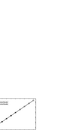
Figure 7: Mean first-passage time $\langle T\rangle_{t}$ versus $t$ on a semilogarithmic scale. The solid line corresponds to the relation between $\langle T\rangle_{t}$ and network order $N_{t}$: $\langle T\rangle_{t}\approx\frac{5}{6}\,N_{t}=\frac{5}{6}\,(2\times 4^{t}+1)$ as given by Eq. (58).

VII Conclusion

In this paper, on the basis of the well-known Koch fractal we have proposed a scale-free network that is called Koch network. We have provided a detailed exact analysis of the topological features. We have shown that the Koch network displays a rich structural behavior: it is simultaneously scale free and small world, and has a high clustering coefficient. In particular, we have shown that the Koch network is an absolutely two-point uncorrelated network. The especial structural characteristics make Koch network unique within the class of scale-free networks.

The uniqueness of the topological features for Koch network presented here makes it potentially interesting to study dynamical processes occurring on the network. We have investigated the random walk process and a particular trapping problem (with a trap located at a hub node) on the Koch network. We have obtained analytically the scaling efficiency exponents which are interesting to random walks. We have shown analytically that the mean first-passage time behaves linearly with the number of network nodes [see Eqs. (41) and (58)], which indicates that despite the presence of loops in the Koch network, the linear scaling of the MFPT for random walks is similar to that of a scale-free tree Bobe05 . Our analytical result confirms a previous conclusion obtained by numerical simulations that for scale-free networks (with loops or not): the MFPT of random walks increases linearly with the network order HuXuWuWa06 ; Bobe05 .

Acknowledgment

We thank Yichao Zhang and Ming Yin for their help. This research was supported by the National Basic Research Program of China under Grant No. 2007CB310806; the National Natural Science Foundation of China under Grants No. 60704044, No. 60873040, and No. 60873070; the Shanghai Leading Academic Discipline Project No. B114, and the Program for New Century Excellent Talents in University of China (Grant No. NCET-06-0376). W L Xie also acknowledges the support provided by Hui-Chun Chin and Tsung-Dao Lee Chinese Undergraduate Research Endowment (CURE).

Appendix A Derivation of the average path length

Figure 8: Second construction method of Koch network that highlights self-similarity. The graph after $t+1$ construction steps, $K(t+1)$, is composed of four copies of $K(t)$ denoted as $K_{t}^{\theta}$ $(\theta=1,2,3,4)$, which are connected to one another as above.

The Koch network has a self-similar structure that allows one to calculate $d_{t}$ analytically. The self-similar structure is obvious from an equivalent network construction method: to obtain $K(t+1)$, one can make four copies of $K(t)$ and join them at the hub nodes. As shown in Fig. 8, network $K(t+1)$ may be obtained by the juxtaposition of four copies of $K(t)$, which are labeled as $K_{t}^{1}$, $K_{t}^{2}$, $K_{t}^{3}$, and $K_{t}^{4}$, respectively. Then we can write the sum $D_{t+1}$ as

$$D_{t+1}=4\,D_{t}+\Delta_{t}\,,$$ (59)

where $\Delta_{t}$ is the sum over all shortest paths whose end points are not in the same $K_{t}$ branch. The solution of Eq. (59) is

$$D_{t}=4^{t-1}D_{1}+\sum_{x=1}^{t-1}4^{t-x-1}\Delta_{x}\,.$$ (60)

The paths that contribute to $\Delta_{t}$ must all go through at least one of the three edge nodes (i.e., $X$, $Y$ and $Z$ in Fig. 8) at which the different $K_{t}$ branches are connected. The analytical expression for $\Delta_{t}$, called the length of crossing paths, is found below.

Denote $\Delta_{t}^{\alpha,\beta}$ as the sum of length for all shortest paths with end points in $K_{t}^{\alpha}$ and $K_{t}^{\beta}$, respectively. If $K_{t}^{\alpha}$ and $K_{t}^{\beta}$ meet at an edge node, $\Delta_{t}^{\alpha,\beta}$ rules out the paths where either end point is that shared edge node. For example, each path contributing to $\Delta_{t}^{1,2}$ should not end at node $X$. If $K_{t}^{\alpha}$ and $K_{t}^{\beta}$ do not meet, $\Delta_{t}^{\alpha,\beta}$ excludes the paths where either end point is any edge node. For instance, each path contributive to $\Delta_{t}^{2,3}$ should not end at node $X$ or $Y$. Then the total sum $\Delta_{t}$ is

$$\Delta_{t}= \,\Delta_{t}^{1,2}+\Delta_{t}^{1,3}+\Delta_{t}^{1,4}+\Delta_{t}^{2,3}+\Delta_{t}^{2,4}+\Delta_{t}^{3,4}.$$ (61)

By symmetry, $\Delta_{t}^{1,2}=\Delta_{t}^{1,3}=\Delta_{t}^{1,4}$ and $\Delta_{t}^{2,3}=\Delta_{t}^{2,4}=\Delta_{t}^{3,4}$, so that

$$\Delta_{t}=3\Delta_{t}^{1,2}+3\Delta_{t}^{2,3}\,.$$ (62)

In order to find $\Delta_{t}^{1,2}$ and $\Delta_{t}^{2,3}$, we define

$$s_{t}=\sum_{\stackrel{{\scriptstyle i\in K(t)}}{{i\neq X}}}d_{iX}\,.$$ (63)

Considering the self-similar network structure, we can easily know that at time $t+1$, the quantity $s_{t+1}$ evolves recursively as

$$s_{t+1} = 2\,s_{t}+\left[s_{t}+(N_{t}-1)\right]+\left[s_{t}+(N_{t}-1)\right]$$ (64)

$$= 4\,s_{t}+4\times 4^{t}.$$

Using $s_{1}=12$, we have

$$s_{t}=4^{t}\,(t+2).$$ (65)

On the other hand, by definition given above, we have

$$\Delta_{t}^{1,2} = \sum_{\begin{subarray}{c}i\in K_{t}^{1},\,\,j\in K_{t}^{2}\\ i,j\neq X\end{subarray}}d_{ij}$$ (66)

$$= \sum_{\begin{subarray}{c}i\in K_{t}^{1},\,\,j\in K_{t}^{2}\\ i,j\neq X\end{subarray}}(d_{iX}+d_{jX})$$

$$= (N_{t}-1)\sum_{\begin{subarray}{c}i\in K_{t}^{1}\\ i\neq X\end{subarray}}d_{iX}+(N_{t}-1)\sum_{\begin{subarray}{c}j\in K_{t}^{2}\\ j\neq X\end{subarray}}d_{jX}$$

$$= 2(N_{t}-1)\sum_{\begin{subarray}{c}i\in K_{t}^{1}\\ i\neq X\end{subarray}}d_{iX}$$

$$= 2(N_{t}-1)\,s_{t},$$

and

$$\Delta_{t}^{2,3} = \sum_{\begin{subarray}{c}i\in K_{t}^{2},\,i\neq X\\ j\in K_{t}^{3},\,j\neq Y\end{subarray}}d_{ij}$$ (67)

$$= \sum_{\begin{subarray}{c}i\in K_{t}^{2},\,i\neq X\\ j\in K_{t}^{3},\,j\neq Y\end{subarray}}(d_{iX}+d_{XY}+d_{jY})$$

$$= 2(N_{t}-1)\,s_{t}+(N_{t}-1)^{2}\,,$$

where $d_{XY}=1$ has been used. Substituting Eqs. (66) and (67) into Eq. (62), we obtain

$$\Delta_{t} = 12(N_{t}-1)\,s_{t}+3\,(N_{t}-1)^{2}\,$$ (68)

$$= (12t+27)\times 16^{t}.$$

Inserting Eq. (68) for $\Delta_{x}$ into Eq. (60) and using $D_{1}=72$, we have

$$D_{t}=\frac{4^{t}}{3}\times\left(2+7\times 4^{t}+6t\times 4^{t}\right).$$ (69)

Inserting Eq. (69) into Eq. (13), one can obtain the analytical expression for $d_{t}$ as shown in Eq. (15).

References

- (1) R. Albert and A.-L. Barabási, Rev. Mod. Phys. 74, 47 (2002).
- (2) S. N. Dorogovtsev and J. F. F. Mendes, Adv. Phys. 51, 1079 (2002).
- (3) M. E. J. Newman, SIAM Rev. 45, 167 (2003).
- (4) S. Boccaletti, V. Latora, Y. Moreno, M. Chavez, and D.-U. Hwanga, Phys. Rep. 424, 175 (2006).
- (5) S. N. Dorogovtsev, A. V. Goltsev and J. F. F. Mendes, Rev. Mod. Phys. 80, 1275 (2008).
- (6) L. da. F. Costa, F. A. Rodrigues, G. Travieso, and P. R. V. Boas, Adv. Phys. 56, 167 (2007).
- (7) A.-L. Barabási and R. Albert, Science 286, 509 (1999).
- (8) D.J. Watts and H. Strogatz, Nature (London) 393, 440 (1998).
- (9) Z. Z. Zhang and S. G. Zhou, Physica A 380, 621 (2007).
- (10) Z. Z. Zhang, L. C. Chen, L. J. Fang, S. G. Zhou, Y. C. Zhang, and J. H. Guan, J. Stat. Mech.: Theory Exp. (2009) P02034.
- (11) R. Albert, H. Jeong, and A.-L. Barabási, Nature (London) 406, 378 (2000).
- (12) D. S. Callaway, M. E. J. Newman, S. H. Strogatz, and D. J. Watts, Phys. Rev. Lett. 85, 5468 (2000).
- (13) R. Cohen, K. Erez, D. ben-Avraham, and S. Havlin, Phys. Rev. Lett. 85, 4626 (2000).
- (14) R. Cohen, K. Erez, D. ben-Avraham, and S. Havlin, Phys. Rev. Lett. 86, 3682 (2001).
- (15) R. Pastor-Satorras and A. Vespignani, Phys. Rev. Lett. 86, 3200 (2001).
- (16) A. Barrat and M. Weigt, Eur. Phys. J. B 13, 547 (2000).
- (17) Z. Z. Zhang, S. G. Zhou, T. Zou, and G. S. Chen, J. Stat. Mech.: Theory Exp. (2008) P09008.
- (18) J. D. Noh and H. Rieger, Phys. Rev. Lett. 92, 118701 (2004).
- (19) V. Sood, S. Redner, and D. ben-Avraham, J. Phys. A: Math. Gen. 38, 109 (2005).
- (20) S. Condamin, O. Bénichou, V. Tejedor, R. Voituriez, and J. Klafter, Nature (London) 450, 77 (2007).
- (21) O. Bénichou, B. Meyer, V. Tejedor, and R. Voituriez, Phys. Rev. Lett. 101, 130601 (2008).
- (22) S. Condamin, V. Tejedor, R. Voituriez, O. Bénichou and J. Klafter, Proc. Natl. Acad. Sci. USA 105, 5675 (2008).
- (23) L. K. Gallos, C. Song, S. Havlin, and H. A. Makse, Proc. Natl. Acad. Sci. USA 104, 7746 (2007).
- (24) A. Baronchelli, M. Catanzaro, and R. Pastor-Satorras, Phys. Rev. E 78, 011114 (2008).
- (25) S. M. Lee, S. H. Yook, and Y. Kim, Physica A 387, 3033 (2008).
- (26) S. Havlin and D. ben-Avraham, Adv. Phys. 36, 695 (1987).
- (27) A. L. Lloyd, and R. M. May, Science, 292, 1316 (2001).
- (28) F. Jasch and A. Blumen, Phys. Rev. E 63, 041108 (2001).
- (29) M. F. Shlesinger, Nature (London) 443, 281 (2006).
- (30) M. E. J. Newman and M. Girvan, Phys. Rev. E 69, 026113 (2004).
- (31) A. G. Cantú and E. Abad, Phys. Rev. E 77, 031121 (2008).
- (32) E. W. Montroll, J. Math. Phys. 10, 753 (1969).
- (33) J. Whitmarsh and Govindjee, Concepts in Photobiology: Photosynthesis and Photomorphogenesis (Narosa, New Delhi, 1999).
- (34) F. Fouss, A. Pirotte, J. M. Renders, and M. Saerens, IEEE Trans. Knowl. Data Eng. 19, 355 (2007).
- (35) R. Metzler and J. Klafter, J. Phys. A: Math. Gen. 37, R161 (2004).
- (36) R Burioni and D Cassi, J. Phys. A: Math. Gen. 38, R45 (2005).
- (37) Z.-G. Huang, X.-J. Xu, Z.-X. Wu, and Y.-H. Wang, Eur. Phys. J. B 51, 549 (2006).
- (38) J. J. Kozak and V. Balakrishnan, Phys. Rev. E 65, 021105 (2002).
- (39) J. J. Kozak and V. Balakrishnan, Int. J. Bifurcation Chaos Appl. Sci. Eng. 12, 2379 (2002).
- (40) E. Agliari, Phys. Rev. E 77, 011128 (2008).
- (41) E. M. Bollt, D. ben-Avraham, New J. Phys. 7, 26 (2005).
- (42) Z. Z. Zhang, Y. C. Zhang, S. G. Zhou, M. Yin, and J. H. Guan, J. Math. Phys. 50, 033514 (2009).
- (43) H. von Koch, Acta Math. 30, 145 (1906).
- (44) A. Lakhtakia, V. K. Varadan, R. Messier, and V. V. Varadan, J. Phys. A: Math. Gen. 20, 3537 (1987).
- (45) B. Mandlebrot, The Fractal Geometry of Nature (Freeman, San Francisco, 1982).
- (46) E. Ravasz and A.-L. Barabási, Phys. Rev. E 67, 026112 (2003).
- (47) M. Hinczewski and A. N. Berker, Phys. Rev. E 73, 066126 (2006).
- (48) Z. Z. Zhang, L. C. Chen, S. G. Zhou, L. J. Fang, J. H. Guan, and T. Zou, Phys. Rev. E 77, 017102 (2008).
- (49) S. Maslov and K. Sneppen, Science 296, 910 (2002).
- (50) R. Pastor-Satorras, A. Vázquez, and A. Vespignani, Phys. Rev. Lett. 87, 258701 (2001).
- (51) M. E. J. Newman, Phys. Rev. Lett. 89, 208701 (2002).
- (52) J. P. K. Doye and C. P. Massen, Phys. Rev. E 71, 016128 (2005).
- (53) Z. Z. Zhang, S. G. Zhou, T. Zou, L. C. Chen, and J. H. Guan, Eur. Phys. J. B 60, 259 (2007).
- (54) A. Vázquez, R. Pastor-Satorras and A. Vespignani, Phys. Rev. E 65, 066130 (2002).
- (55) J. J. Ramasco, S. N. Dorogovtsev, and R. Pastor- Satorras, Phys. Rev. E 70, 036106 (2004).
- (56) R. D. Hughes, Random Walks: Random Walks and Random Environments (Clarendon, Oxford, 1995), Vol. 1.
- (57) J.S. Andrade Jr., H.J. Herrmann, R.F.S. Andrade and L.R. da Silva, Phys. Rev. Lett. 94, 018702 (2005).
- (58) Z.Z. Zhang, F. Comellas, G. Fertin and L.L. Rong, J. Phys. A: Math. Gen. 39, 1811 (2006).
- (59) Z. Z. Zhang, L. L. Rong, and S. G. Zhou, Phys. Rev. E, 74, 046105 (2006).
- (60) Z. Z. Zhang, J. H. Guan, W. L. Xie, Y. Qi, and S. G. Zhou, EPL, 86, 10006 (2009).
- (61) C. N. Kaplan, M. Hinczewski, and A. N. Berker arXiv: 0811.3437.
- (62) S.N. Dorogovtsev, A.V. Goltsev, J.F.F. Mendes, Phys. Rev. E 65, 066122 (2002).
- (63) F. Comellas, G. Fertin, A. Raspaud, Phys. Rev. E 69, 037104 (2004).
- (64) Z. Z. Zhang, S. G. Zhou, and L. C. Chen, Eur. Phys. J. B 58, 337 (2007).
- (65) Z. Z. Zhang, L. L. Rong, S. G. Zhou, Physica A 377, 329 (2007).
- (66) H. D. Rozenfeld, S. Havlin, and D. ben-Avraham, New J. Phys. 9, 175 (2007).
- (67) Z. Z. Zhang, Y. Qi, S. G. Zhou, W. L. Xie, and J. H. Guan, Phys. Rev. E 79, 021127 (2009).
- (68) M. Giona, Chaos, Solitons Fractals 7, 1371 (1996).
- (69) J. G. Kemeny and J. L. Snell, Finite Markov Chains (Springer, New York, 1976).