Clifford Algebra with Mathematica

1 Introduction

The importance of Clifford algebra was recognized for the first time in quantum field theory. Lately, there has been a tendency to exploit their power in many others fields. These fields include projective geometry [10], electrodynamics [12], analysis on manifolds and differential geometry [9], crystallography [19, 3] to name a few. A recent account of the applications of Clifford algebra in fields such as robotics, computer vision, computer graphics, engineering, neural and quantum computing, etc., can be found in [4] and [20].

General introductions to Clifford algebra can be found in several books (see for instance Refs. [18] and [5]). Here, a gently introduction to the Clifford algebra of $\mathbb{R}^{n}$ is presented together with some examples to show the generality of this algebra in order to provide a general language comprising vectors, complex numbers and quaternions. The main goal is to implement the basic operations of Clifford algebras in Mathematica, resulting in a package for doing Clifford algebra computations. There exists some other packages and specialized programs for doing Clifford algebra; CLIFFORD/Bigebra is a Maple package which include additional specialized packages such as SchurFkt (for the Hopf Algebra of Symmetric Functions) and GfG - Groebner for Grassmann (for Computing Groebner Bases for Ideals in Grassmann Algebra) [2]; TCliffordAlgebra is as add-on application for the Mathematica package Tensorial that implements Clifford algebra operations [17]; CLICAL is a stand-alone calculator-type computer program for MS-DOS [16]. While the first two packages requires more specialized knowledge of Clifford algebras, CLICAL and the package presented here is easy to use and can be used by non mathematicians. More recently, Clifford Multivector Toolbox, a toolbox for computing with Clifford algebras in MATLAB, has been released [7]. A more specialized package is GAViewer package, designed for computation and visualization of objects in conformal geometric algebra [6] (for a more recent account and application see Ref. [13]). We must emphasise that with the exception of the Maple packages, the other packages and toolboxes only allow numeric computations. Our Clifford Mathematica package allow us to carry out numerical and symbolic computations with complex numbers, quaternions, the hyperbolic plane, Grassmann algebra and, Dirac and Pauli algebras, all defined within the Clifford algebra framework. Our package clifford.m is available for download at:

https://github.com/jlaragonvera/Geometric-Algebra

2 The Clifford algebra of $\mathbb{R}^{n}$

The set of n-tuples of the form $(x_{1},x_{2},...,x_{n})$ with the standard operations of addition and multiplication for real numbers is a vector space, over the field of real numbers, which we denote as $\mathbb{R}^{n}$. It means that the addition of $n$-tuples, and multiplication by real numbers satisfy certain properties which are those of a vector space [14]. The canonical basis of $\mathbb{R}^{n}$ is the set of $n$-dimensional vectors $\{{\mathbf{e}}_{1},{\mathbf{e}}_{2},...,{\mathbf{e}}_{n}\}$ where $\langle{\mathbf{e}}_{i},{\mathbf{e}}_{j}\rangle=\delta_{ij}$ and $\langle\;,\;\rangle$ is a inner product in $\mathbb{R}^{n}$. An element ${\mathbf{v}}$ of $\mathbb{R}^{n}$ is written as a linear combination of this canonical basis:

$$v=x_{1}{\mathbf{e}}_{1}+x_{2}{\mathbf{e}}_{2}+\cdots+x_{n}{\mathbf{e}}_{n}.$$

It is said therefore that the n-tuple $(x_{1},x_{2},...,x_{n})$ is the coordinate vector of ${\mathbf{v}}$ with respect to the canonical basis $\{{\mathbf{e}}_{1},{\mathbf{e}}_{2},...,{\mathbf{e}}_{n}\}$.

The vector space $\mathbb{R}^{n}$ has two operations defined: addition of vectors and multiplication of vectors by scalars. The multiplication by vectors between themselves is not defined. The algebraic structure which considers multiplication between vectors is called an algebra.

An algebra ${\mathcal{A}}$ is a vector space over a field ${\mathcal{F}}$ together with a binary multiplication $\mathbf{ab}$ in ${\mathcal{A}}$ such that form any ${\mathbf{a}},{\mathbf{b}},{\mathbf{c}}\in{\mathcal{A}}$ and $\alpha\in{\mathcal{F}}$ [11]:

$$({\mathbf{a}}+{\mathbf{b}}){\mathbf{c}} = \mathbf{ac}+\mathbf{bc}$$

$${\mathbf{a}}({\mathbf{b}}+{\mathbf{c}}) = \mathbf{ab}+\mathbf{ac}$$

$$\alpha(\mathbf{ab}) = (\alpha{\mathbf{a}}){\mathbf{b}}={\mathbf{a}}(\alpha{\mathbf{b}}).$$

In the case of the vector space $\mathbb{R}^{n}$, the field ${\mathcal{F}}$ is the set of real numbers. In order to construct an algebra from $\mathbb{R}^{n}$, it is required to define a product $\mathbf{ab}$ between vectors in $\mathbb{R}^{n}$. One particular product in $\mathbb{R}^{n}$ can be defined as follows.

Let us consider the vector space $\mathbb{R}^{n}$ with the inner product $\langle{\mathbf{a}},{\mathbf{b}}\rangle$ and an orthonormal basis $\{{\mathbf{e}}_{1},{\mathbf{e}}_{2},...,{\mathbf{e}}_{n}\}$. We construct an algebra from $\mathbb{R}^{n}$ by introducing a product between vectors in $\mathbb{R}^{n}$ that satisfies the condition

$$\mathbf{ab}+\mathbf{ba}=2\langle{\mathbf{a}},{\mathbf{b}}\rangle{\mathbf{1}},$$ (1)

where ${\mathbf{1}}$ is the identity of the algebra. The product so defined is associative:

$${\mathbf{a}}(\mathbf{bc})=(\mathbf{ab}){\mathbf{c}},$$

and we are constructing an algebra ${\mathcal{A}}$ equipped with an identity ${\mathbf{1}}$.

With the vector space and the product (1), the resulting algebra of all possible sums and products of vectors in $\mathbb{R}^{n}$ is called the Clifford algebra of $\mathbb{R}^{n}$ and is denoted by ${\mathcal{C}l}_{n}$. Note in particular that

$${\mathbf{a}}^{2} = \langle{\mathbf{a}},{\mathbf{a}}\rangle$$

$${\mathbf{e}}_{i}^{2} = {\mathbf{1}}$$ (2)

$${\mathbf{e}}_{i}{\mathbf{e}}_{j} = -{\mathbf{e}}_{j}{\mathbf{e}}_{i},\;\;\;\;i\neq j.$$

The Clifford algebra ${\mathcal{C}l}_{n}$ is itself a vector space of dimension $\sum_{p=0}^{n}{\binom{n}{p}}=2^{n}$, with basis

$$\left\{1,{\mathbf{e}}_{1},\ldots,{\mathbf{e}}_{n},{\mathbf{e}}_{1}{\mathbf{e}}_{2},\ldots,{\mathbf{e}}_{1}{\mathbf{e}}_{n},\ldots,{\mathbf{e}}_{1}{\mathbf{e}}_{2}\cdots{\mathbf{e}}_{n}\right\},$$

such that an element ${\mathcal{A}}$ in ${\mathcal{C}l}_{n}$ is written as

$$A = a_{0}+a_{11}{\mathbf{e}}_{1}+\cdots+a_{1i}{\mathbf{e}}_{n}+a_{21}{\mathbf{e}}_{1}{\mathbf{e}}_{2}+$$ (3)

$$+\cdots a_{2i}{\mathbf{e}}_{1}{\mathbf{e}}_{n}+\cdots+a_{di}{\mathbf{e}}_{1}{\mathbf{e}}_{2}\cdots{\mathbf{e}}_{n},$$

where $d=2^{n}-1$ and $i={\binom{n}{p}}$ for the real numbers $a_{pi}$. Consequently, the vector space ${\mathcal{C}l}_{n}$ can be decomposed in $n+1$ subspaces as:

$${\mathcal{C}l}_{n}=\Lambda^{0}\mathbb{R}^{n}\oplus\Lambda^{1}\mathbb{R}^{n}\oplus\cdots\oplus\Lambda^{n}\mathbb{R}^{n}.$$ (4)

Each subspace is of dimension ${\binom{n}{p}}$.

The elements ${\mathcal{A}}$ (Eqn. 3) of the Clifford algebra ${\mathcal{C}l}_{n}$ are called multivectors, and those of $\Lambda^{p}\mathbb{R}^{n}$, $p$-vectors. In particular, $0$-vectors are real numbers and $\dim(\Lambda^{0}\mathbb{R}^{n})=1$. $\Lambda^{1}\mathbb{R}^{n}$ has the basis $\{{\mathbf{e}}_{1},{\mathbf{e}}_{2},\ldots,{\mathbf{e}}_{n}\}$, so $1$-vectors are simply vectors and $\dim(\Lambda^{1}\mathbb{R}^{n})=n$. $\Lambda^{2}\mathbb{R}^{n}$ has the basis $\{{\mathbf{e}}_{1}{\mathbf{e}}_{2},{\mathbf{e}}_{1}{\mathbf{e}}_{3},\ldots,{\mathbf{e}}_{1}{\mathbf{e}}_{n}\}$ and their elements ($2$-vectors) are also called bivectors. Finally, $\Lambda^{n}\mathbb{R}^{n}$ has as basis $\{{\mathbf{e}}_{1}{\mathbf{e}}_{2}\cdots{\mathbf{e}}_{n}\}$ and since $\dim(\Lambda^{n}\mathbb{R}^{n})=1$, the $n$-vectors of ${\mathcal{C}l}_{n}$ are referred as pseudoscalars.

In this paper, arbitrary multivectors will be denoted by non bold upper case characters without ornamentation such as $A$. $p$-vectors will be denoted by $A_{p}$, with the exception of vectors ($1$-vectors), that will be denoted by bold lower case characters such as ${\mathbf{a}}$.

Bearing in mind that the decomposition of the vector space ${\mathcal{C}l}_{n}$ as the direct sum of the subspaces $\Lambda^{p}\mathbb{R}^{n}$, $0\leq p\leq n$, given in (4), any multivector $A$ can be written as

$$A=\langle A\rangle_{0}+\langle A\rangle_{1}+\cdots+\langle A\rangle_{n},$$ (5)

where $\langle A\rangle_{p}$, the $p$-vector part of $A$, is the projection of $A\in{\mathcal{C}l}_{n}$ into $\Lambda^{p}\mathbb{R}^{n}$. $\langle\;\;\rangle$ is called the grade operator.

2.1 Innner and outer products

Given the decomposition (4), an important property of a Clifford algebra is the existence of products that allows us to move from one subspace of ${\mathcal{C}l}_{n}$ to another. Let us first consider the product of two $1$-vectors. For all $\mathbf{u},\mathbf{v}\in\Lambda^{1}\mathbb{R}^{n}$, their product $\mathbf{u}\mathbf{v}$ can be written as

$$\mathbf{u}\mathbf{v}=\frac{1}{2}\left(\mathbf{u}\mathbf{v}+\mathbf{v}\mathbf{u}\right)+\frac{1}{2}\left(\mathbf{u}\mathbf{v}-\mathbf{v}\mathbf{u}\right).$$

Now define the “inner” and “outer” products as follows

$$\mathbf{u}\cdot\mathbf{v} = \frac{1}{2}\left(\mathbf{u}\mathbf{v}+\mathbf{v}\mathbf{u}\right)=\langle{\mathbf{a}},{\mathbf{b}}\rangle,$$

$$\mathbf{u}\wedge\mathbf{v} = \frac{1}{2}\left(\mathbf{u}\mathbf{v}-\mathbf{v}\mathbf{u}\right).$$

The inner product is symmetric and notice that vectors $\mathbf{u}$ and $\mathbf{v}$ are orthogonal if an only if $\mathbf{u}\mathbf{v}=-\mathbf{v}\mathbf{u}$. The outer product $\mathbf{u}\wedge\mathbf{v}$ is antisymmetric (and associative) and vanishes whenever the two vectors are collinear, that is, $\mathbf{u}$ and $\mathbf{v}$ are collinear (or linearly dependent) if an only if $\mathbf{u}\mathbf{v}=\mathbf{v}\mathbf{u}$. Thus, the product $\mathbf{u}\mathbf{v}$ provides information about the relative directions of the vectors. Anticommutativity means orthogonality and commutativity means collinearity. Notice that for the bases vectors of $\mathbb{R}^{n}$, we have

$$\mathbf{e}_{i}\mathbf{e}_{j} = \mathbf{e}_{i}\wedge\mathbf{e}_{j},\;\;\;i\neq j,$$

$$\mathbf{e}_{i}\cdot\mathbf{e}_{i} = \mathbf{e}_{i}^{2}=1.$$

From the following equality

$$\mathbf{u}\mathbf{v} = \mathbf{u}\cdot\mathbf{v}+\mathbf{u}\wedge\mathbf{v},$$

$$= \langle\mathbf{u}\mathbf{v}\rangle_{0}+\langle\mathbf{u}\mathbf{v}\rangle_{2},$$

we can extend the notions of inner and outer product to the case of $p$- and $q$-vectors in the following way. For a $p$-vector $A_{p}\in\Lambda^{p}\mathbb{R}^{n}$ and a $q$-vector $B_{q}\in\Lambda^{q}\mathbb{R}^{n}$, the inner product $A_{p}\cdot B_{q}$ is defined by

$$A_{p}\cdot B_{q}=\left\{\begin{array}[]{ll}\left\langle A_{p}B_{q}\right\rangle_{\left|p-q\right|}&\text{if}\quad p,q>0,\\ 0&\text{if}\quad p=0\text{ or }q=0.\end{array}\right.$$ (6)

Analogously, the outer product $A_{p}\wedge B_{q}$ is defined by

$$A_{p}\wedge B_{q}=\left\langle A_{p}B_{q}\right\rangle_{p+q}.$$ (7)

Since arbitrary multivectors can be decomposed as in (5), inner and outer product can be extended by linearity to ${\mathcal{C}l}_{n}$. Then, given $A,B\in{\mathcal{C}l}_{n}$, we have

$$A\cdot B=\sum_{k,l=1}^{n}\langle A\rangle_{k}\cdot\langle B\rangle_{l},$$

$$A\wedge B=\sum_{k,l=1}^{n}\langle A\rangle_{k}\wedge\langle B\rangle_{l},$$

2.2 Geometric interpretation

Bivectors have an interesting geometric interpretation. Just as a vector describes an oriented line segment, with the direction of the vector representing the oriented line and the magnitude of the vector, the length of the segment; a bivector ${\mathbf{a}}\wedge{\mathbf{b}}$ describes an oriented plane segment, with the direction of the bivector representing the oriented plane and the magnitude of the bivector measuring the area of the plane segment (Figure 1). The same interpretation is extended to high-order terms: ${\mathbf{a}}\wedge{\mathbf{b}}\wedge{\mathbf{c}}$ represents an oriented volume. In general, multivectors contain information about orientation of subspaces.

2.3 The main involution

The magnitude or modulus of a multivector $A$ is defined by the equation

$$\left|A\right|=\left\langle\widetilde{A}A\right\rangle_{0}^{1/2},$$ (8)

where $\sim$ denotes the operation reverse defined as

$$\left({\mathbf{e}}_{1}{\mathbf{e}}_{2}\cdots{\mathbf{e}}_{p}\right)^{\sim}={\mathbf{e}}_{p}\cdots{\mathbf{e}}_{2}{\mathbf{e}}_{1}.$$

The operation reverse is distributive [9] so that the reverse of an arbitrary multivector $A$ can be easily calculated. If the inverse of a multivector $A$ exists, it is denoted by $A^{-1}$ or ${\mathbf{1}}/A$, and is defined by the equation $AA^{-1}={\mathbf{1}}$.

2.4 General metrics

In many physical applications one considers real vector spaces $\mathbb{R}^{n}$ with metrics that are not positive definite with the bilinear form $\langle\;,\;\rangle$, in (1), such that

$$\langle{\mathbf{x}},{\mathbf{x}}\rangle=x_{1}^{2}+x_{2}^{2}+\cdots+x_{p}^{2}-x_{p+1}^{2}-\cdots-x_{p+q}^{2},$$

where $n=p+q$. In this case, the vector space is denoted as $\mathbb{R}^{p,q}$, giving rise to the Clifford algebra ${\mathcal{C}l}_{p,q}$. Using the orthonormal basis $\{{\mathbf{e}}_{1},{\mathbf{e}}_{2},\ldots,{\mathbf{e}}_{n}\}$ of $\mathbb{R}^{p,q}$, the relations (2) are now:

$${\mathbf{e}}_{i}^{2} = {\mathbf{1}}\;\;\;\;1<i\leq p$$

$${\mathbf{e}}_{i}^{2} = -{\mathbf{1}}\;\;\;\;p<i\leq n$$ (9)

$${\mathbf{e}}_{i}{\mathbf{e}}_{j} = -{\mathbf{e}}_{j}{\mathbf{e}}_{i},\;\;\;\;i\neq j.$$

The scalar $p$ is called the signature of the bilinear form $\langle\;,\;\rangle$.

3 Clifford algebra calculations with Mathematica

According to Eqns. (6), (7) and (8), all that we should need to manipulate multivectors in a computer algebra program such as Mathematica, would be to define the two basic operations: geometric product and grade operator. In the first case, a simple algorithm for the computation of the geometric product between multivectors can be devised by noticing that a general multivector (3) in ${\mathcal{C}l}_{p,q}$ is formed by a linear combination of terms in the form

$${\mathbf{e}}_{1}^{m_{1}}{\mathbf{e}}_{2}^{m_{2}}\cdots{\mathbf{e}}_{n}^{m_{n}},$$ (10)

where $m_{i}=1,0$, $(i=1,...,n)$. Let us call blades to multivectors of the form (10). The geometric product of two of these blades is:

$$\left({\mathbf{e}}_{1}^{m_{1}}{\mathbf{e}}_{2}^{m_{2}}\cdots{\mathbf{e}}_{n}^{m_{n}}\right)\left({\mathbf{e}}_{1}^{r_{1}}{\mathbf{e}}_{2}^{r_{2}}\cdots{\mathbf{e}}_{n}^{r_{n}}\right)=$$

$$\qquad(-1)^{s}{\mathbf{e}}_{1}^{m_{1}+r_{1}}{\mathbf{e}}_{2}^{m_{2}+r_{2}}\cdots{\mathbf{e}}_{n}^{m_{n}+r_{n}},$$ (11)

where the sum $m_{i}+r_{i}$ is evaluated modulus two, and

$$s=\sum\limits_{1\leq i<j\leq n}r_{i}m_{j}.$$

If $m_{i}+r_{i}=2$ then, in order to have the right hand side in the form (10) when considering the signature of the bilinear form, ${\mathbf{e}}_{i}^{m_{i}+r_{i}}$ will be replaced with $\langle{\mathbf{e}}_{i},{\mathbf{e}}_{i}\rangle{\mathbf{e}}_{i}^{0}$, and in this case we have:

$${\mathbf{e}}_{1}^{m_{1}+r_{1}}\cdots{\mathbf{e}}_{i}^{m_{i}+r_{i}}\cdots{\mathbf{e}}_{n}^{m_{n}+r_{n}}=$$

$$\qquad\langle{\mathbf{e}}_{i},{\mathbf{e}}_{i}\rangle{\mathbf{e}}_{1}^{m_{1}+r_{1}}\cdots{\mathbf{e}}_{i}^{0}\cdots{\mathbf{e}}_{n}^{m_{n}+r_{n}}.$$

Equation (10) enables us to establish an isomorphism between blades and n-tuples $(m_{1},m_{2},...,m_{n})$ that can be manipulated more easily from a computational point of view. The grade of a blade such as (10) is simply $m_{1}+m_{2}+\cdots+m_{n}$.

If, in Mathematica code, we denote the $j$-th basis vector ${\mathbf{e}}_{j}$ as e[j], a blade such as ${\mathbf{e}}_{1}{\mathbf{e}}_{3}{\mathbf{e}}_{4}$, ( ${\mathbf{e}}_{1}^{1}{\mathbf{e}}_{2}^{0}{\mathbf{e}}_{3}^{1}{\mathbf{e}}_{4}^{1}$ using the nomenclature of Eqn. 10) is written as:

$$\verb|e[1]e[3]e[4]|,$$ (12)

and can be internally represented simply by $(1,0,1,1)$. Care must be taken in preserving the canonical order of the expression, since for instance e[1]e[3] is a geometric product of two vectors and e[1]e[3] $\neq$ e[3]e[1].

Let us consider the Clifford algebra ${\mathcal{C}l}_{p,q}$. If dim $=p+q$ is the dimension of the vector space, the following Mathematica code implements the transformation of a blade onto a $n$-tuple:

ntuple[x_, dim_]:=
     ReplacePart[Table[0,{dim}],1,List @@
                           x /. e[k_]->{k}]

The signature of the bilinear form can be set by using $SetSignature = p. Relations (2.4) can be coded as:

bilinearform[e[i_],e[i_]]:=
        If[i <= $SetSignature, 1, -1]

With some exceptions, it is not necessary to define the dimension of the vector space since it can be calculated directly. The maximum dimension of the space where a blade is embedded can be extracted from the list:

dimensions[x_]:=
    List @@ x /. e[k_?Positive] -> k

and, therefore, enables us to perform computations in any dimension with any given signature. For a general multivector, we need the relations that include the distributivity of addition:

dimensions[x_Plus]:=
   List @@ Distribute[tmp[x]] /.
                        tmp -> dimensions
dimensions[a_]:=
   {0} /; FreeQ[a,e[_?Positive]]
dimensions[a_ x_]:=
   dimensions[x] /; FreeQ[a,e[_?Positive]]

From (3), the geometric product between two blades with a bilinear form of signature p can therefore be evaluated with geoprod:

geoprod[x_,y_]:= Module[{q=1,s,r={}},
  p1= ntuple[x, Max[dimensions[x],
               dimensions[y]]],
  p2= ntuple[y, Max[dimensions[x],
               dimensions[y]]],
  s= Sum[p2[[m]]*p1[[n]],
   {m,Length[p1]-1},{n,m+1,Length[p2]}];
  r1=p1+p2;
  r=Mod[p1+p2,2];
  Do[
    If[r1[[i]]==2,
     q*=bilinearform[e[i],e[i]]];
    If[r[[i]]==1, q*=e[i]],
  {i, Length[r]}];
    (-1)^s*q ]

The latter function evaluates the geometric product of two blades in a Clifford algebra ${\mathcal{C}l}_{p,q}$. One step further consists in to calculate the geometric product of two arbitrary multivectors such as (3). This can be achieved from geoprod by providing the transformation rules which contains the properties of the geometric product under multiplication of blades by real numbers and addition of blades. Here is the behavior under scalar multiplication:

geoprod[a_,y_]:=
   a y /; FreeQ[a,e[_?Positive]]
geoprod[x_,a_]:=
   a x /; FreeQ[a,e[_?Positive]]
geoprod[a_ x_,y_]:=
   a geoprod[x,y] /; FreeQ[a,e[_?Positive]]
geoprod[x_,a_ y_]:=
   a geoprod[x,y] /; FreeQ[a,e[_?Positive]]

and the distributivity of addition:

geoprod[x_, y_Plus]:=
   Distribute[tmp[x,y,p],Plus] /.
                        tmp -> geoprod
geoprod[x_Plus, y_]:=
   Distribute[tmp [x,y,p],Plus] /.
                        tmp -> geoprod

Therefore, the function to calculate the geometric product of arbitrary multivectors is defined as

GeometricProduct[_]:= $Failed
GeometricProduct[m1_,m2_,m3__]:=
    tmp[ GeometricProduct[m1,m2],m3] /.
                tmp -> GeometricProduct
GeometricProduct[m1_,m2_]:=
    geoprod[Expand[m1], Expand[m2]]

To complete the basic operations of a Clifford algebra, we must define and implement the grade operator. The following auxiliary function calculates the grade of a blade

gradblade[a_]:=
     0 /; FreeQ[a,e[_?Positive]]
gradblade[x_]:=
     Plus @@ ntuple[x, Max[dimensions[x]]]
gradblade[a_ x_]:=
     gradblade[x] /; FreeQ[a,e[_?Positive]]

Now, Grade[x,n] should extract the term of grade $n$ from the multivector $X$. Firstly, we consider the case when the multivector $X$ is a blade of grade $r$: $\langle X\rangle_{n}=0$ if $r\neq n$ and $\langle X\rangle_{n}=X$ if $r=n$. The code reads:

Grade[x_, n_?NumberQ]:=
                  If[gradblade[x]==n,x,0]]

For a general multivector $X$, we have:

Grade[x_Plus, n_?NumberQ]:=
  Distribute[tmp[x,n],Plus] /. tmp -> Grade

Functions GeometricProduct and Grade enable us to construct all the operations which can be defined in a Clifford algebra, such as outer product (OuterProduct[v,w,..]), inner product (InnerProduct[v,w,..]), magnitude (Magnitude[v]), reverse (Turn[v]}), inverse (MultivectorInverse[v]), dual (Dual[v,dim]), and many others, all included in the package Clifford.m. This package works with general multivectors of the form (3), but particular cases can help to envisage the power of multivector calculus, as it is made explicit in what follows.

4 Vectors

Let us consider the Clifford algebra ${\mathcal{C}l}_{p,0}$. $n$-dimensional vectors are $1$-vectors and lie in the subspace $\Lambda^{1}\mathbb{R}^{p,0}$. A vector ${\mathbf{a}}$ is therefore ${\mathbf{a}}=\langle A\rangle_{1}$, where $A$ is a general multivector.

The inner product defined in (6) becomes now the standard “dot product”  between vectors. The “cross product”  ${\mathbf{a}}\times{\mathbf{b}}$ of vector calculus is defined in $\mathbb{R}^{3}$ and is related to the outer product of vectors ${\mathbf{a}}$ and ${\mathbf{b}}$. The vector ${\mathbf{a}}\times{\mathbf{b}}$ is perpendicular to ${\mathbf{a}}\wedge{\mathbf{b}}$ and with the same magnitude: $\left|{\mathbf{a}}\wedge{\mathbf{b}}\right|=\left|{\mathbf{a}}\times{\mathbf{b}}\right|$. The explicit algebraic relation between them is [8]:

$${\mathbf{a}}\times{\mathbf{b}}=(-{\mathbf{e}}_{1}{\mathbf{e}}_{2}{\mathbf{e}}_{3})({\mathbf{a}}\wedge{\mathbf{b}}),$$ (13)

where ${\mathbf{e}}_{1}{\mathbf{e}}_{2}{\mathbf{e}}_{3}$ is the pseudoscalar of ${\mathcal{C}l}_{3,0}$. We may actually take this as a definition of the cross product.

From (13), it is easy to define the function crossprod[v,w] that gives the cross product between two three-dimensional vectors ${\mathbf{v}}$ and ${\mathbf{w}}$:

crossprod[v_,w_]:=
      GeometricProduct[-e[1]e[2]e[3],
                         OuterProduct[v,w]]

The associativity property of the geometric product allows algebraic manipulations typical of real numbers that are not possible in the Gibbs’ vector algebra since the cross and dot products are not generally associative. For example

$${\mathbf{a}}\times({\mathbf{b}}\times{\mathbf{c}})\neq({\mathbf{a}}\times{\mathbf{b}})\times{\mathbf{c}}.$$

Even more, many products such as ${\mathbf{a}}\cdot({\mathbf{b}}\cdot{\mathbf{c}})$ are not even defined. With Clifford algebra all products are not only well defined but associative making simpler many algebraic manipulations and allowing to define derivatives and integrals just as they are defined for real functions of real variables, provided that we are careful to maintain the order of the factors since geometric product is not commutative.

One specific example that shows the simplicity of some expressions if the geometric product is used, is concerning rotations. Consider a vector ${\mathbf{v}}$ in $\mathbb{R}^{n}$ which is rotated by an angle $\theta$ in the oriented plane characterized by the bivector ${\mathbf{a}}\wedge{\mathbf{b}}$. After the rotation, the vector ${\mathbf{v}}$ is transformed into ${\mathbf{v}}^{\prime}$, given by [8]:

$${\mathbf{v}}=\widetilde{U}{\mathbf{v}}U,$$ (14)

where

$$U=\cos(\theta/2)+\frac{{\mathbf{a}}\wedge{\mathbf{b}}}{\left|{\mathbf{a}}\wedge{\mathbf{b}}\right|}\sin(\theta/2).$$

The direction of the rotation (clockwise or counter clockwise) is specified by the orientation of the bivector ${\mathbf{a}}\wedge{\mathbf{b}}$. Eqn. 14 gives the rotated vector ${\mathbf{v}}^{\prime}$ regardless of the dimension of the space in which it is embedded. No corresponding simple expression exists in vector algebra.

As an example, which can be easily visualized, consider the vector ${\mathbf{v}}=(1,1,1)$, to be rotated $90^{o}$ maintaining invariant the plane $xy$. To characterize the plane $xy$, we can use ${\mathbf{a}}\wedge{\mathbf{b}}$ where ${\mathbf{a}}=(1,0,0)$ and ${\mathbf{b}}=(0,1,0)$, in which case we get a rotation counterclockwise and is easy to see that ${\mathbf{v}}^{\prime}=(-1,1,1)$, but if we use ${\mathbf{b}}\wedge{\mathbf{a}}$ then the rotation is clockwise and ${\mathbf{v}}^{\prime}=(1,-1,1)$. Here is this example solved with Clifford:

In[1]:= << Clifford.m
In[2]:= v = e[1]+e[2]+e[3];
In[3]:= plane = OuterProduct[e[1],e[2]]/
         Magnitude[OuterProduct[e[1],e[2]]]
Out[3]= e[1]e[2]

The operator $U$ is now defined ($\widetilde{U}$ is the reverse of $U$):

In[4]:= u = Cos[Pi/4] + plane Sin[Pi/4];
In[5]:= vprime = GeometricProduct[Turn[u],
                     GeometricProduct[v,u]]
Out[5]= -e[1]+e[2]+e[3]

So we get a counterclockwise rotation where the vector ${\mathbf{v}}=(1,1,1)$ becomes ${\mathbf{v}}^{\prime}=(-1,1,1)$. The implementation in Mathematica of this rotation is the function Rotation[v,a,b].

5 Drawing multivectors in the 3-dimensional space.

The elements of the Clifford algebra ${\mathcal{C}l}_{3,0}$ can be visualized in the $3$-dimensional space, providing geometrical insights. The package include a function to draw multivectors belonging to ${\mathcal{C}l}_{3,0}$, called GADraw, that will be described in what follows.

GADraw includes embedded functions to draw vectors, bivectors and the pseudoscalar of ${\mathcal{C}l}_{3,0}$. For example let us draw the multivector ${\mathbf{e}}_{3}+{\mathbf{e}}_{1}{\mathbf{e}}_{2}+{\mathbf{e}}_{2}{\mathbf{e}}_{3}+{\mathbf{e}}_{1}{\mathbf{e}}_{2}{\mathbf{e}}_{3}$:

In[1]:= << Clifford.m
In[2]:= A = e[3] + e[1]e[2] +
                     e[2]e[3]+e[1]e[2]e[3];
In[3]:= GADraw[A];
Out[3]=

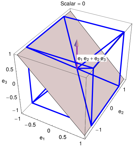
Figure 1: A vector, a bivector (plane) and the pseudoscalar (cube) drawn with the aid of the function GADraw.

The result is shown in Fig. 1. The bivector is represented by an area and the pseudoscalar as a scalable cube. In the particular case of the vector $(0,0,1)$, the arrow in its tip was generated by the following code [23]:

mat[1] = Sin[t]*(e[1]/14)+Cos[t]*(e[2]/14),
mat[2] = Sin[t+0.25]*(e[1]/14) +
                     Cos[t+0.25]*(e[2]/14),
mat[3] = e[3]/5,

This arrow is then translated and rotated (in this case to the tip of the vector $(0,0,1)$) with the aid of the function Rotation[mat,w,p], where $w=e_{3}$ and $p$ is the vector that points the site where the tip of the arrow must be located. If sc=Sqrt[p[[1]]^2 +p[[2]]^2 +p[[3]]^2]/2 is a scale factor then all this procedure can be encoded as:

If[OuterProduct[ToBasis[p], e[3]] === 0,
cone =
 Table[Array[ToVector[mat[#],3] &,3] +
   p-ToVector[mat[3],3],{t,0.25,2*Pi,0.25}],
elms =
 Array[sc*ToVector[Grade[Rotation[
         mat[#],e[3], ToBasis[p]],1],3]&,3];
cone=
 Table[elms+p-res[[3]],{t,0.25,2*Pi,0.25}]];

 arrow = Graphics3D[{FaceForm[color],
              EdgeForm[], Polygon /@ cone}]

Where ToBasis and ToVector are functions, defined on the same package Clifford; the former changes from the coordinates of a vector to the basis notation (12) and the last one does the opposite.

We must emphasize that the above code was included with the aim to show that symmetry operations, rotations in this case, can be carried out by using the elements of the Clifford algebra without requiring matrices. This algebra provides a consistent computational framework with significant applications in computer graphics, vision and robotics [6].

6 Complex numbers

Let us consider the Clifford algebra of the most simple space that has a geometrical structure: the plane $\mathbb{R}^{2,0}$. Taking the canonical basis $\{{\mathbf{e}}_{1},{\mathbf{e}}_{2}\}$, a basis for the Clifford algebra ${\mathcal{C}l}_{2,0}$ is $\{{\mathbf{1}},{\mathbf{e}}_{1},{\mathbf{e}}_{2},{\mathbf{e}}_{1}{\mathbf{e}}_{2}\}$ and a general multivector $A\in{\mathcal{C}l}_{2,0}$ has the form

$$A=k_{0}+k_{1}{\mathbf{e}}_{1}+k_{2}{\mathbf{e}}_{2}+k_{3}{\mathbf{e}}_{1}{\mathbf{e}}_{2}.$$

We can decompose ${\mathcal{C}l}_{2,0}$ as ${\mathcal{C}l}_{2,0}={\mathcal{C}l}_{2,0}^{+}\oplus{\mathcal{C}l}_{2,0}^{-}$, such that ${\mathcal{C}l}_{2,0}^{+}$ contains even grade elements and ${\mathcal{C}l}_{2,0}^{-}$ contains odd grade elements. Therefore, $A$ can be expressed as the sum of two multivectors: $A=A^{+}+A^{-}$, where $A^{+}\in{\mathcal{C}l}_{2,0}^{+}$ and $A^{-}\in{\mathcal{C}l}_{2,0}^{-}$. That is

$$A = A^{+}+A^{-},$$

$$A^{+} = k_{0}+k_{3}{\mathbf{e}}_{1}{\mathbf{e}}_{2},$$

$$A^{-} = k_{1}{\mathbf{e}}_{1}+k_{2}{\mathbf{e}}_{2}.$$

We focus our attention into ${\mathcal{C}l}_{2,0}^{+}$; it is itself an algebra so that it is called the even subalgebra of ${\mathcal{C}l}_{2,0}$. By taking

$${\mathbf{i}}={\mathbf{e}}_{1}{\mathbf{e}}_{2},$$ (15)

an element of ${\mathcal{C}l}_{2,0}^{+}$ can be written as

$$z=k_{0}+k_{3}{\mathbf{i}}.$$

Since ${\mathbf{i}}^{2}=({\mathbf{e}}_{1}{\mathbf{e}}_{2})({\mathbf{e}}_{1}{\mathbf{e}}_{2})=-({\mathbf{e}}_{1}{\mathbf{e}}_{2}{\mathbf{e}}_{2}{\mathbf{e}}_{1})=-1$, and ${\mathbf{i}}$ is itself a generator of rotations [8], we see that ${\mathcal{C}l}_{2,0}^{+}$ is equivalent to the algebra of complex numbers.

The algebraic operations of complex numbers can therefore be worked out with Clifford. In order to get a more standard notation we firstly define the function

In[6]:= transform[x]:= x /. i -> e[1]e[2]

which makes the identification (15). Here we have two complex numbers:

In[7]:= w = a + b i;
In[8]:= z = c + d i;

The product $(a+b{\mathbf{i}})(c+d{\mathbf{i}})$ becomes

In[9]:= GeometricProduct[transform[w],
             transform[z]] /. e[1]e[2] -> i
Out[9]:= a c - b c + b c i + a d i

The equivalence between some built-in basic operations of complex numbers in Mathematica and those of a Clifford algebra defined the package is shown in the following table:

Built-in Objects	Clifford.m Objects
Re[z]	Grade[z,0]
Im[z]	GeometricProduct[
	Grade[z,2],-e[1]e[2]]
Conjugate[z]	Turn[z]
Abs[z]	Magnitude[z]

The inverse of the complex number $w$ can be calculated with MultivectorInverse:

In[10]:= MultivectorInverse[transform[w]]
                           /. e[1]e[2] -> i

           a - bi
Out[10]= ----------
            2    2
           a  + b

7 Quaternions

Extending from the previous section, we now develop the Clifford algebra of $\mathbb{R}^{3,0}$, equipped with the canonical basis $\{{\mathbf{e}}_{1},{\mathbf{e}}_{2},{\mathbf{e}}_{3}\}$. The Clifford algebra ${\mathcal{C}l}_{3,0}$ is an eighth-dimensional vector space with the basis $\{{\mathbf{1}},{\mathbf{e}}_{1},{\mathbf{e}}_{2},{\mathbf{e}}_{3},{\mathbf{e}}_{1}{\mathbf{e}}_{2},{\mathbf{e}}_{2}{\mathbf{e}}_{3},{\mathbf{e}}_{1}{\mathbf{e}}_{3},{\mathbf{e}}_{1}{\mathbf{e}}_{2}{\mathbf{e}}_{3}\}$. A general multivector $A\in{\mathcal{C}l}_{3,0}$ is written as

$$A = k_{0}+k_{1}{\mathbf{e}}_{1}+k_{2}{\mathbf{e}}_{2}+k_{3}{\mathbf{e}}_{3}+k_{4}{\mathbf{e}}_{1}{\mathbf{e}}_{2}+$$

$$k_{5}{\mathbf{e}}_{2}{\mathbf{e}}_{3}+k_{6}{\mathbf{e}}_{1}{\mathbf{e}}_{3}+k_{7}{\mathbf{e}}_{1}{\mathbf{e}}_{2}{\mathbf{e}}_{3},$$

which can be also expressed as $A=A^{+}+A^{-}$, where

$$A^{+} = k_{0}+k_{4}{\mathbf{e}}_{1}{\mathbf{e}}_{2}+k_{5}{\mathbf{e}}_{2}{\mathbf{e}}_{3}+k_{6}{\mathbf{e}}_{1}{\mathbf{e}}_{3}$$

$$A^{-} = k_{1}{\mathbf{e}}_{1}+k_{2}{\mathbf{e}}_{2}+k_{3}{\mathbf{e}}_{3}+k_{7}{\mathbf{e}}_{1}{\mathbf{e}}_{2}{\mathbf{e}}_{3}.$$

The even-grade elements $A^{+}$ form the subalgebra ${\mathcal{C}l}_{3,0}^{+}$ of ${\mathcal{C}l}_{3,0}$, equivalent to the algebra of quaternions. Hence, we have:

$${\mathbf{i}} = -{\mathbf{e}}_{2}{\mathbf{e}}_{3},$$

$${\mathbf{j}} = {\mathbf{e}}_{1}{\mathbf{e}}_{3}$$ (16)

$${\mathbf{k}} = -{\mathbf{e}}_{1}{\mathbf{e}}_{2},$$

leading to the famous equations

$${\mathbf{i}}^{2} = {\mathbf{j}}^{2}={\mathbf{k}}^{2}=-1,$$ (17)

$$\mathbf{ijk} = -1.$$

With the identifications given in (7), an element of ${\mathcal{C}l}_{3,0}^{+}$ can be written now as

$$Q=q_{0}+q_{1}{\mathbf{i}}+q_{2}{\mathbf{j}}+q_{3}{\mathbf{k}},$$

which, in view of the properties (17), is a quaternion.

The algebra of quaternions is therefore comprised in the same package. The basic operations of this algebra are carried out by the function already defined, such as GeometricProduct, MultivectorInverse, Magnitude and Turn. To simplify the operations, we have incorporated the definitions (7) and redefined some functions to work only with quaternions and complex numbers. The new functions begin with the word Quaternion, namely, QuaternionProduct, QuaternionInverse, QuaternionMagnitude and QuaternionTurn. So, for instance the inverse of the quaternion $q=a+3{\mathbf{i}}+6{\mathbf{j}}-10{\mathbf{k}}$ is

In[11]:= q = a + 3 i + 6 j - 10 k;
In[12]:= QuaternionInverse[q]

         a - 3 i - 6 j + 10 k
Out[12]= ---------------------
                     2
              145 + a

8 Grassmann algebra

The outer product (OuterProduct) defined in (7) is associative and the identity ${\mathbf{1}}$, in a Clifford algebra ${\mathcal{C}l}_{n,0}$, is also the identity for the outer product. Consequently, the vector space $\mathbb{R}^{p,0}$ with the outer product already defined is an algebra of dimension $2^{n}$, which is called the Grassmann algebra of $\mathbb{R}^{p,0}$. Notice that it does not depend on the inner product of the vector space, but just on the alternation of the outer product.

Grassmann algebra has relevance in modern theoretical physics [15] and has the right structure for the theory of determinants. The structure of this algebra contained in Clifford algebra allows us to reformulate Grassmann calculus [15], and to give an extensive treatment of determinants [9], both in terms of Clifford algebra.

9 The hyperbolic plane

Perhaps the simplest example of a problem involving non positive definite metrics is the Minkowsky model of the hyperbolic plane. Here we shall develop some basic ideas and calculations just to give a flavor of this kind of application of Clifford algebra and the use of the package Clifford for non positive definite metrics. In the next section, one extra dimension is introduced and the resulting algebras have great relevance in relativity theory and quantum mechanics.

One can always visualize a surface of constant positive Gaussian curvature $1/R^{2}$ (see for instance [21] for concepts related to differential geometry) as a sphere, with radius $R$, embedded in a three dimensional Euclidean space. The surface is described by the equation $x_{1}^{2}+x_{2}^{2}+x_{3}^{2}=R^{2}$. A surface of constant negative curvature, however, cannot be embedded in a Euclidean space, so alternative possibilities must be developed to visualize such surfaces. The simplest surface of constant negative curvature is often called the hyperbolic plane, the Bolyai-Lobachevsky plane, or the pseudosphere. This surface can be globally embedded in a space equipped with the Minkowsky metrics instead of the Euclidean one. A three-dimensional Minkowsky space can be identified by the fact that if $(x_{1},x_{2},x_{3})$ are the coordinates of a vector ${\mathbf{x}}$ in this space, then the distance to the origin is $\left|x\right|^{2}=x_{1}^{2}+x_{2}^{2}-x_{3}^{2}$.

The equation

$$x_{1}^{2}+x_{2}^{2}-x_{3}^{2}=-R^{2},$$ (18)

defines a hyperboloid of two sheets intersecting the $x_{3}$ axis at the points $\pm 1$. Either sheet (upper or lower) models an infinite surface without a boundary (the Minkowsky metric becomes positive definite upon it) that, as we shall see, has constant Gaussian curvature $-1/R^{2}$.

We can easily convince ourselves that ${\mathcal{C}l}_{2,1}$ is indeed the three-dimensional Minkowsky space (the signature of the bilinear form is $2$). We shall proceed to calculate the Gaussian curvature of the hyperboloid (18) with the standard formulas of differential geometry but with the metrics of ${\mathcal{C}l}_{2,1}$. In three dimensions, the Gaussian curvature of a surface $f(x_{1},x_{2},x_{3})=0$ can be written as [22]:

$$k=\frac{1}{2}\left[{\mathbf{n}}\cdot\nabla^{2}{\mathbf{n}}+\left(\nabla\cdot{\mathbf{n}}\right)^{2}\right],$$

where ${\mathbf{n}}=\nabla f(x_{1},x_{2},x_{3})/\left|\nabla f(x_{1},x_{2},x_{3})\right|$ is the normal to the surface. In a three-dimensional space with metrics non positive definite, the gradient of a scalar function $\phi$ and the divergence and Laplacian of a vector function ${\mathbf{f}}=(f_{1},f_{2},f_{3})$ are defined as

$$\nabla\phi = ({\mathbf{e}}_{1}\cdot{\mathbf{e}}_{1})\frac{\partial\phi}{\partial x_{1}}{\mathbf{e}}_{1}+({\mathbf{e}}_{2}\cdot{\mathbf{e}}_{2})\frac{\partial\phi}{\partial x_{2}}{\mathbf{e}}_{2}+$$

$$({\mathbf{e}}_{3}\cdot{\mathbf{e}}_{3})\frac{\partial\phi}{\partial x_{3}}{\mathbf{e}}_{3},$$

$$\nabla\cdot{\mathbf{f}} = ({\mathbf{e}}_{1}\cdot{\mathbf{e}}_{1})^{2}\frac{\partial f_{1}}{\partial x_{1}}+({\mathbf{e}}_{2}\cdot{\mathbf{e}}_{2})^{2}\frac{\partial f_{2}}{\partial x_{2}}+$$

$$({\mathbf{e}}_{3}\cdot{\mathbf{e}}_{3})^{2}\frac{\partial f_{3}}{\partial x_{3}},$$

$$\nabla^{2}{\mathbf{f}} = \left[({\mathbf{e}}_{1}\cdot{\mathbf{e}}_{1})^{3}\frac{\partial^{2}}{\partial x_{1}^{2}}+({\mathbf{e}}_{2}\cdot{\mathbf{e}}_{2})^{3}\frac{\partial^{2}}{\partial x_{2}^{3}}+\right.$$

$$\left.({\mathbf{e}}_{3}\cdot{\mathbf{e}}_{3})^{3}\frac{\partial^{2}}{\partial x_{3}^{2}}\right]\left(f_{1}{\mathbf{e}}_{1}+f_{2}{\mathbf{e}}_{2}+f_{3}{\mathbf{e}}_{3}\right).$$

We can use Clifford to evaluate all these expressions:

In[1]:= << Clifford.m

The adequate metrics is defined

In[2]:= $SetSignature = 2

Here are the differential operators:

In[3]:= var = {x1,x2,x3};
In[4]:= GeoGrad[g_]:=
         Sum[InnerProduct[e[k],e[k]]
           *D[g,var[[k]]]*e[k],{k,3}]
In[5]:= GeoDiv[v_]:=
         Sum[InnerProduct[e[k],e[k]]^2
           D[Coeff[v,e[k]],var[[k]]],{k,3}]
In[6]:= GeoLap[v_]:=
         Sum[(InnerProduct[e[k],e[k]]^3)*
           D[v,{var[[k]],2}],{k,3}]

The function Coeff[m,b], extracts the coefficient of the blade b in the multivector m. The surface and their normal are:

In[7]:= f := x1^2 + x2^2 - x3^2 + R^2;
In[8]:= norm = GeoGrad[f] /
                     Magnitude[GeoGrad[f]];

and, finally, the Gaussian curvature is:

In[9]:= kGauss =
          (InnerProduct[norm,GeoLap[norm]]+
           (GeoDiv[norm])^2)/2  // Simplify

                 1
Out[9]= --------------------
            2     2     2
          x1  + x2  - x3

Points in the surface fulfills:

In[10]:= x3 = Sqrt[x1^2 + x2^2 + R^2],

and therefore:

In[11]:= kGauss

           -2
Out[11]= -R

which is the Gaussian curvature of the hyperboloid.

Some considerations concerning the isometries (distance-preserving transformations) of the hyperbolic plane are pertinent before leaving this section. Like the Euclidean ones, the isometries of the hyperbolic plane can be described in terms of reflections about given axes. All these isometries have simple expressions in terms of Clifford algebra. For instance, Eqn. (14) for rotations in a given plane remains valid in ${\mathcal{C}l}_{2,1}$ but now is called a Lorentz transformation. In general, given the vectors ${\mathbf{u}}_{1},{\mathbf{u}}_{2},\ldots,{\mathbf{u}}_{k}$ in ${\mathcal{C}l}_{p,q}$, such that $({\mathbf{u}}_{1},{\mathbf{u}}_{2},\ldots,{\mathbf{u}}_{k})({\mathbf{u}}_{k},{\mathbf{u}}_{k-1},\ldots,{\mathbf{u}}_{1})=1$, the transformation

$${\mathbf{v}} \longmapsto (-1)^{k}({\mathbf{u}}_{k}{\mathbf{u}}_{k-1}\cdots{\mathbf{u}}_{1}){\mathbf{v}}({\mathbf{u}}_{1}{\mathbf{u}}_{2}\cdots{\mathbf{u}}_{k})$$

$$=(-1)^{k}\widetilde{U}{\mathbf{v}}U,$$

is an isometry [9]. If $k$ is even, the isometry is a rotation, if $k$ is odd, it is a reflection [3]. Now, if $q=0$ ($\in{\mathcal{C}l}_{p,q}$), transformations such as the previous one are orthogonal. For $q=1$ (as the case of the Minkoswky space) they are Lorentz transformations.

10 Dirac and Pauli algebras

Now let us add one extra dimension to the space of the previous example and consider ${\mathcal{C}l}_{3,1}$. This vector space is fifteen-dimensional with basis

$$\left\{\mathbf{1},\mathbf{e}_{1},\mathbf{e}_{2},\mathbf{e}_{3},\mathbf{e}_{4},\mathbf{e}_{1}\mathbf{e}_{2},\mathbf{e}_{1}\mathbf{e}_{3},\mathbf{e}_{1}\mathbf{e}_{4},\mathbf{e}_{2}\mathbf{e}_{3},\mathbf{e}_{2}\mathbf{e}_{4},\mathbf{e}_{3}\mathbf{e}_{4},\right.$$

$$\left.\mathbf{e}_{1}\mathbf{e}_{2}\mathbf{e}_{3},\mathbf{e}_{1}\mathbf{e}_{3}\mathbf{e}_{4},\mathbf{e}_{2}\mathbf{e}_{3}\mathbf{e}_{4},\mathbf{e}_{1}\mathbf{e}_{2}\mathbf{e}_{3}\mathbf{e}_{4}\right\}.$$

The basis vectors $\mathbf{e}_{i}$ satisfy the relations:

$${\mathbf{e}}_{1}^{2}={\mathbf{e}}_{2}^{2}={\mathbf{e}}_{3}^{2}={\mathbf{1}},\;\;\;\;{\mathbf{e}}_{4}^{2}=-{\mathbf{1}},$$

which is the algebra of the Dirac matrices in relativistic quantum theory. Due to this isomorphism, ${\mathcal{C}l}_{3,1}$ is often referred as the Dirac algebra.

The even subalgebra ${\mathcal{C}l}_{3,1}^{+}$ has a basis $\{{\mathbf{1}},{\mathbf{e}}_{1}{\mathbf{e}}_{2},{\mathbf{e}}_{1}{\mathbf{e}}_{3},{\mathbf{e}}_{1}{\mathbf{e}}_{4},{\mathbf{e}}_{2}{\mathbf{e}}_{3},{\mathbf{e}}_{2}{\mathbf{e}}_{4},{\mathbf{e}}_{3}{\mathbf{e}}_{4},{\mathbf{e}}_{1}{\mathbf{e}}_{2}{\mathbf{e}}_{3}{\mathbf{e}}_{4}\}$ and is equivalent to the algebra of the Pauli matrices used in quantum mechanics of spin-$\frac{1}{2}$ particles. This can be seen with the identifications

$$\sigma_{1}={\mathbf{e}}_{1}{\mathbf{e}}_{4},\;\;\;\sigma_{2}={\mathbf{e}}_{2}{\mathbf{e}}_{4},\;\;\;\sigma_{3}={\mathbf{e}}_{3}{\mathbf{e}}_{4}.$$

By taking ${\mathbf{i}}={\mathbf{e}}_{1}{\mathbf{e}}_{2}{\mathbf{e}}_{3}{\mathbf{e}}_{4}=\sigma_{1}\sigma_{2}\sigma_{3}$, we get

$$\sigma_{i}^{2} = {\mathbf{1}},\;\;\;i=1,2,3$$

$$\sigma_{1}\sigma_{2} = {\mathbf{i}}\sigma_{3}$$

$$\sigma_{2}\sigma_{3} = {\mathbf{i}}\sigma_{1}$$

$$\sigma_{3}\sigma_{1} = {\mathbf{i}}\sigma_{2},$$

which are the familiar Pauli matrix relations. ${\mathcal{C}l}_{3,1}^{+}$ is also called the Pauli algebra.

Following the same reasoning, we can prove that the even subalgebra of the Pauli algebra is isomorphic to the quaternions. The even subalgebra of the quaternions is isomorphic to the complex numbers. The even subalgebra of the complex numbers is $\mathbb{R}$.

11 Conclusion

The basic ideas of the Clifford algebra of a vector space are presented and a Mathematica package for calculations within this algebra is developed and demonstrated for complex numbers, quaternions, the hyperbolic plane, Grassmann algebra and, Dirac and Pauli algebras. The relevance of Clifford algebra in physics and mathematics lies in the fact that it provides a complete algebraic framework of geometric concepts such as directed lines, areas, volumes, etc. (For this reason, Clifford algebra is also referred as Geometric algebra [9]). Quantities such as vectors, complex numbers, quaternions, Pauli and Dirac matrices, have been normally described by physicists with a mixture of disjoint mathematical systems. All of them are naturally contained in a Clifford algebra. It becomes therefore an efficient mathematical language in a vast domain of physics. Future work comprises extending our Mathematica package to other high-level programming languages in order to facilitate its adoption within the community.

Acknowledgements:  JLA wishes to thank UNAM-DGAPA-PAPIIT for financially support this research through grant IN106115.

References:

- [1]
- [2] R. Abłamowicz and B. Fauser. Clifford/bigebra, a maple package for clifford (co)algebra computations, 2007. ©1996-2007, RA&BF. Available at www.math.tntech.edu/rafal/.
- [3] G. Aragón-González, J.L. Aragón, and M.A. Rodríguez. The decomposition of an orthogonal transformation as a product of reflections. J. Math. Phys. 47, 2006, Art. No. 013509 (10 pages).
- [4] E. Bayro-Corrochano and G. Sobczyk. Geometric Algebra with Applications in Science and Engineering. Birkhauser, Boston 2001.
- [5] R. Delanghe, F. Sommen, and V. Soucek. Clifford Algebra and Spinor-Valued Functions. D. Reidel Publishing Co., Holland 1992.
- [6] L. Dorst, D. Fontijne, and S. Mann. Geometric Algebra for Computer Science: An Object-Oriented Approach to Geometry. Morgan Kauffman, San Francisco, CA 2007.
- [7] S. Sangwine, and E. Hitzer. Clifford Multivector Toolbox: A toolbox for computing with Clifford algebras in Matlab. http://clifford-multivector-toolbox.sourceforge.net. Created June 22, 1025. Last accessed December 1, 2015.
- [8] D. Hestenes. New Fundations for Classical Mechanics. D. Reidel Publishing Co., Holland 1987.
- [9] D. Hestenes and G. Sobczyk. Clifford Algebra to Geometric Calculus. A unified Language for Mathematics and Physics. D. Reidel Publishing Co., Holland 1985.
- [10] D. Hestenes and R. Ziegler. Projective geometry with clifford algebra. Acta Appl. Math., 23, 1991, 25–63.
- [11] N. Jacobson. Lectures in Abstract Algebra II: Linear Algebra. Springer, New York 1984.
- [12] B. Jancewicz. Multivectors and Clifford Algebra in Electrodynamics. World Scientific, Singapore 1988.
- [13] K. Kanatani. Understanding Geometric Algebra: Hamilton, Grassmann, and Clifford for Computer Vision and Graphics. A K Peters/CRC Press, Florida 2015.
- [14] S. Lang. Linear Algebra. Addison-Wesley, New York 1969.
- [15] A. Lasenby, C. Doran, and S. Gull. Grassmann calculus, pseudoclassical mechanics, and geometric algebra. J. Math. Phys. 34, 1993, pp. 3683–3712.
- [16] P. Lounesto. Clifford Algebras and Spinors. Cambridge University Press, Cambridge, 2001.
- [17] D. Park, R. Cabrera, and J.-F. Gouyet. Tensorial 4.0 - a mathematica package for tensor calculus. MiER 12, 2097, pp. 109–122.
- [18] Ian Porteous. Clifford Algebras and the Classical Groups. Cambridge University Press, Cambridge, 1995.
- [19] M.A. Rodríguez, J.L. Aragón, and L. Verde-Star. Clifford algebra approach to the coincidence problem for planar lattices. Acta Crystallogr. A 61, 2005, pp. 173–184.
- [20] G. Sommer. Geometric Computing with Clifford Algebras Theoretical Foundations and Applications in Computer Vision and Robotics. Springer, Heidelberg 2001.
- [21] D.J. Struik. Differential Geometry. Addison-Wesley, New York 1961.
- [22] C.E. Weatherburn. Differential Geometry of Three Dimensions. Vol. 1. Cambridge University Press, Cambridge 1965.
- [23] T. Wickam-Jones. Mathematica Graphics: Techniques & Applications. Springer –Verlag, New York 1994.