Elastic theory of unconstrained non-Euclidean plates

Abstract

Non-Euclidean plates are a subset of the class of elastic bodies having no stress-free configuration. Such bodies exhibit residual stress when relaxed from all external constraints, and may assume complicated equilibrium shapes even in the absence of external forces. In this work we present a mathematical framework for such bodies in terms of a covariant theory of linear elasticity, valid for large displacements. We propose the concept of non-Euclidean plates to approximate many naturally formed thin elastic structures. We derive a thin plate theory, which is a generalization of existing linear plate theories, valid for large displacements but small strains, and arbitrary intrinsic geometry. We study a particular example of a hemispherical plate. We show the occurrence of a spontaneous buckling transition from a stretching dominated configuration to bending dominated configurations, under variation of the plate thickness.

1 Introduction

Elasticity theory, in its most fundamental formulations, describes the statics and dynamics of three-dimensional (3D) elastic bodies. Such “fundamental” models are extremely complex, due to both high dimensionality and nonlinearity. This intrinsic complexity has motivated over the years the development of simplified, or reduced models of elasticity. In particular, models of lower spatial dimension have been developed to describe the mechanics of slender bodies, such as columns, shells and plates. These models are based on various approximations, such as lateral inextensibility, small deflections and small deformations. In particular, the Kirchhoff-Love assumptions [1] allow the derivation of reduced two-dimensional (2D) theories of plates. The Föppl-Von Kármán (FVK) plate equations are one of the successful reduced descriptions of plates mechanics. It expresses the elastic energy of a deformed elastic plate as a sum of stretching and bending energies of a 2D surface. The stretching energy, which accounts for in-plane deformations, is linear in the plate thickness, $h$. The bending energy, which depends on the curvature of the deformed plate, is cubic in $h$. Other reduced 2D theories usually bear the same structure, i.e., their energy is given by the sum of a stretching term and a bending term [2]. The validity of the dimensional reduction from 3D to 2D models, based on the Kirchhoff-Love assumptions, has been the subject of many scientific disputes [3]. Recently, the FVK theory has been derived from a 3D elastic theory by means of an asymptotic expansion [4]. The stretching and bending terms in the FVK theory have also been derived as two different vanishing thickness $\Gamma$-limits of the 3D elastic energy [5].

2D elastic theories distinguish between two types of thin bodies: plates and shells. Plates are elastic bodies that bear no structural variation across their thin dimension, and possess a planar rest configuration. Shells are elastic bodies that bear structural variations across their thin dimension, and as a result, possess a non-planar rest configuration. In both cases the postulated existence of a stress-free, rest configuration is of paramount importance.

Recent technological developments have extended the range of mechanical structures that can be engineered and constructed. Plates of nanometer scale thickness can be manufactured [12], responsive nano-structures are being developed [13, 14], and the use of shape memory materials that lead to large shape transformations has been extended [15]. In addition, the application of mechanics to biological systems, such as in the study of plant mechanics and motility [16] and the study of mechanically induced cell differentiation [17], is a rapidly developing field. Such developments have renewed the interest in elasticity. Several recent theoretical works have focused on the onset of various mechanical instabilities and the scaling of the generated patterns [12, 18], and other thoroughly analyzed the assumptions underlying some of the dimensionally reduced models [5].

The modeling of growing elastic bodies is an area in which current theories of elasticity face difficulties. Growing tissues, such as leaves, exhibit very complex configurations even in the absence of external forces [6]. Although leaves (and many other growing tissues) are relatively thin (compared to their lateral dimensions), there are no reduced 2D elastic theories that model their shaping mechanisms. Another class of systems for which current theories do not apply are elastic bodies undergoing irreversible plastic deformations. The main difficulty in applying elasticity theory to growing bodies, or elastic bodies having undergone plastic deformations, is their lack of a stress-free configuration. Specifically, in most models, the elastic energy density of a deformed body depends on the local elastic modulus and the strain tensor. The latter is defined by the gradient of the mapping between a stress-free configuration and the deformed configuration. It can be shown, for example, that a general growth process of an elastic material leads to a body that has no stress-free configuration, thus exhibiting residual stress in the absence of external loading [7].

To formulate an elastic theory for bodies that do not have stress-free configurations, one needs an alternative definition of the strain tensor. At present, certain 3D formulations use the concepts of virtual configuration [8, 9] and intermediate configuration [19, 20] to describe natural growth processes as well as plastic deformations leading to residual stress. The growth process in these theories is decomposed into a growth step, which maps a stress-free configuration into a virtual configuration, and an elastic relaxation step, which maps the virtual configuration into an elastic equilibrium configuration that contains residual stress. These theories use a multiplicative decomposition of the deformation gradient into an elastic and a plastic part. Other theories decompose the strain tensor additively [21].

In the current work, we focus on the elastic response of the body after its “rest configuration” has been modified either by growth, or by plastic deformation. We do not consider the thermodynamic limitations on plastic deformations (which are not relevant to naturally growing tissue). We assume that the distorted “rest configuration” (or virtual configuration) is a known quantity. If an elastic body is capable of assuming the virtual configuration, then there exists a stress-free configuration, which is unique; the solution to the elastic problem is then trivial. If, however, no elastic body can assume the virtual configuration, then no stress-free configuration exists, and we face a non-trivial problem which exhibits residual stress. We term such bodies as “non-Euclidean” because their internal geometry is not immersible in three-dimensional Euclidean space.

We consider now two model examples of elastic structures that belong to the class of systems we have termed non-Euclidean plates, and discuss qualitatively some of their properties. Consider an elastic square slab of lateral dimensions $2L$, and thickness $h$. Suppose we cut out from it a square segment of dimension $L$, leaving out a U-shaped structure (see Figure 1.1$a$). Next, the square is replaced by a trapezoid that has three edges of equal length $L$, and a fourth edge of longer size $L^{\prime}$. Of course, the trapezoid is too large to fit in the square slot. Suppose, however, that we forcefully insert the trapezoid into the slot, gluing its three sides of length $L$ to the corresponding edges of the U-shape. As a result, the U-shape will slightly open, whereas the trapezoid will experience compression. This plane-stress configuration is shown schematically in Figure 1.1$b$. If the plates are sufficiently thin, the trapezoid is unable to sustain the compression and buckles out of plane to form a shape qualitatively described in Figure 1.1$c$.

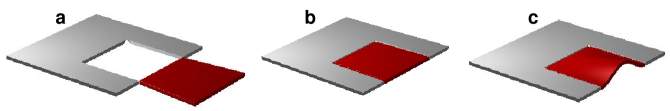
Figure 1.1: Schematic illustration of an unconstrained plate exhibiting residual stress. (a) The two elements composing the plate are shown side by side. (b) As the red trapezoid is too large to fit into the square opening, it is compressed. (c) For a plate sufficiently thin, the induced compression exceeds the buckling threshold, and the trapezoid buckles out of plane . Note that there are many shapes that preserve all lengths along the faces of the plate, yet they cannot be planar.

We note the following points for this toy problem:

1. The three dimensional metric that describes the rest lengths of the compound body (U-shape plus trapezoid) is continuous.

2. If $x^{3}$ denotes the vertical coordinate (say, the distance from the bottom face), then all $x^{3}=const$ surfaces are identical. It is this property that causes the body to remain flat (for sufficiently thick samples), and will later be used to rigorously define non-Euclidean plates.

3. The body exhibits residual stress in the absence of external constraints: in Figure 1.1$b$ the body is in a state of non-trivial plane-stress, identical for all $x^{3}=const$ sections. In the buckled state (Figure 1.1$c$) symmetry is broken. The upper surface is longer then the lower surface, hence at least one of them must be strained. It may easily be shown that the compound body has no unstressed configuration.

4. The problem is purely geometric: As both pieces (the confining U and the trapezoid) are made of the same material, the stiffness of the material (Young’s modulus) has no effect on the equilibrium shape, and we expect to see the same behavior for metals and rubbers (as long as the strains are sufficiently small and the stresses are below the yield stress).

5. The toy problem presented here may easily be solved numerically using commercial software (In fact, a very similar problem was addressed experimentally and analytically in [24]). The treatment used for solving such problems is limited to discrete geometric incompatibilities: two (or more) regular elastic problems that are coupled through their boundary conditions are solved simultaneously. Plastic deformations and non-homogeneous growth processes, however, cannot be mapped into such discrete geometries.

Recent experiments in torn plastic sheets [22] and environmentally responsive gel discs [23] have attracted attention to a specific class of non-Euclidean elastic bodies: thin bodies whose shaping mechanism is essentially two-dimensional. Growing leaves display such behavior, as their growth is believed to be nearly homogeneous across their thin dimension, and inhomogeneous in the lateral dimensions. The gel discs reported in [23] mimic a growing thin 3D body shaped by a 2D growth process. In these experiments initially flat stress-free objects shrink according to a pre-determined chemical gradient in their composition. The shrinking is homogeneous across the thickness, but inhomogeneous in the lateral directions (see Figure 1.2 for an example). The resulting body shows no structural variation across its thin dimension, yet the lateral equilibrium distances, specified by the differential shrinking, define a 2D non-Euclidean metric tensor. Thus, they cannot be preserved in any flat configuration of the disc. Such bodies may not be considered as plates (due to their non-planar intrinsic geometry), nor as shells (as there are no structural variations across the thin dimension). We name such bodies non-Euclidean plates.

The configurations of non-Euclidean plates in the absence of external forces are not flat (Figure 1.2$c$ and 1.2$d$), and may exhibit multi-scale, and fractal-like configurations [22, 23]. Finite element simulations devised to describe such bodies [10, 11], were able to obtain such multi-scale configurations as energy minima. In both computational and theoretical works, it was assumed that the elastic energy can be written as a sum of bending and stretching terms. The bending was measured with respect to a locally flat configuration (as in the FVK plate model), and the stretching was evaluated with respect to a reference 2D metric tensor. None of these works, however, was backed up with a theoretical justification for such assumptions.

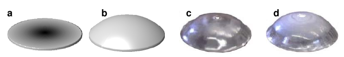
Figure 1.2: An initially flat disc shrinking differentially. (a) The peripheral areas (light grey) shrink significantly, while the center of the disc (dark grey) shrinks moderately. (b) In order to accommodate the center of the disc within the “too short” peripheral ring, the plate must buckle out of plane. While the newly prescribed lateral lengths are satisfied on average (over the thickness), the symmetry breaking causes the upper surface to be tensed, while the lower surface is compressed. (c-d) Experimental realization of non-Euclidean plates, using environmentally responsive gels as described in [23]. The differential shrinkage prescribes a two dimensional geometry of constant positive Gaussian curvature $K=0.11$cm^-2. The thicknesses of the gels are $h_{c}=0.75$mm and $h_{d}=0.6$mm.

In the present work we derive a reduced 2D elastic theory for non-Euclidean plates and discuss their characteristics. The derivation starts from a model of a 3D covariant “incompatible” elasticity, that is, a model for 3D bodies whose intrinsic metric cannot be immersed in a 3D Euclidean space. We advocate that the common definition of strains with respect to a stress-free configuration is too restrictive. Instead, strains can be measured with respect to a reference metric tensor, which is not necessarily immersible in 3D Euclidean space (incompatibility). When the strain tensor is defined with respect to a metric tensor, growth (or any other metric prescription) is naturally decoupled from the elastic relaxation. The second Cauchy-Piola stress tensor (which is linear in the strain for small strains), may be written explicitly in terms of the difference between two metric tensors. In such a formulation residual stress appears inevitably as a result of the lack of immersibility. .

We apply this formulation to thin elastic plates, using the Kirchhoff-Love assumptions. When applied to ordinary plates, our theory coincides with the Koiter plate theory [2]. As in the FVK and Koiter theories, the energy of the plate is a sum of stretching and bending terms. The bending term is cubic in $h$ and quadratic in surface curvatures. The stretching term is linear in $h$ and depends on the difference between the 2D metric tensor of the configuration and the reference metric $\bar{g}$, (in [10] it was termed “target metric”) The covariant elasticity formulation, together with the bending term measures deviations from a flat configuration, while the stretching term measures deviations from the 2D reference metric (which may be non-flat). The resulting model is simple to use, and has an intuitive structure, which clarifies the underlying physics. We end this paper with an application of the theory to a simple case of a hemispherical plate.

2 Theoretical framework: covariant linear elasticity theory

In this section we derive the energy functional of a three-dimensional elastic body as a function of its metric using general curvilinear coordinates. We will show that the energy functional takes the following form,

$$E(g)=\int_{\mathcal{D}}w(g)\sqrt{|\bar{g}|}dx^{1}dx^{2}dx^{3}\qquad w={\textstyle\frac{1}{2}}A^{ijkl}\varepsilon_{ij}\varepsilon_{kl},$$

where we use the Einstein summation convention and

$$A^{ijkl}=\lambda\bar{g}^{ij}\bar{g}^{kl}+\mu\left(\bar{g}^{ik}\bar{g}^{jl}+\bar{g}^{il}\bar{g}^{jk}\right)\qquad\varepsilon_{ij}={\textstyle\frac{1}{2}}\left(g_{ij}-\bar{g}_{ij}\right).$$ (2.1)

Here $g_{ij}$ is the metric tensor, $\bar{g}_{ij}$ is a symmetric positive-definite tensor, which we term the reference metric, and $\lambda,\mu$ are elasticity (Lamè) constants; for tensors $|\cdot|$ denotes the determinant. This energy functional neglects terms that are of order higher than quadratic in $\varepsilon_{ij}$, which is the deviation of the metric from the reference metric. For bodies which possess a stress-free configuration, $\bar{g}$ may be called the rest metric and must comply with six additional differential constraints (the vanishing of the Ricci curvature tensor). Precise definitions will be provided in the following subsections. For a thorough treatment of bodies that have a stress-free configuration, the reader is referred to the recent introductory book by Ciarlet [25], which contains the mathematical background to the subject. A similar treatment, which we consider as a starting point for our generalization, can be found in Koiter [2]. We derive the energy functional in a slightly different manner, yet we try as far as possible to use the notations of [2], later adopted in [25].

2.1 “Incompatible” covariant three-dimensional elasticity

When a body (a compact domain $\Omega\subset\mathbb{R}^{3}$) is endowed with a regular set of material curvilinear coordinates $\boldsymbol{x}=(x^{1},x^{2},x^{3})$, it is also endowed with an induced metric tensor. Specifically, if $\boldsymbol{r}$ denotes the mapping from the domain of parametrization, $\mathcal{D}\subset\mathbb{R}^{3}$, into $\Omega$ (we call $\boldsymbol{r}$ the configuration of the body), then the endowed metric is $g_{ij}=\partial_{i}\boldsymbol{r}\cdot\partial_{j}\boldsymbol{r}$. Here and below we use roman lower-case letters $,i,j,\dots$ for indices $\{1,2,3\}$; the operator $\partial_{i}$ denotes the partial derivative with respect to $x^{i}$. Any deformation of the body (carrying the coordinates along with every material point) will result in a different metric tensor. A rigidity theorem states that if the induced metrics of two configurations $\boldsymbol{r}(\boldsymbol{x})\in\Omega$ and $\tilde{\boldsymbol{r}}(\boldsymbol{x})\in\tilde{\Omega}$ satisfy $g_{ij}(\boldsymbol{x})=\tilde{g}_{ij}(\boldsymbol{x})$ for every $\boldsymbol{x}\in\mathcal{D}$, then the two configurations can only differ by a rigid motion (a uniform translation and a rigid rotation). Thus, the metric (provided that it is immersible in $\mathbb{R}^{3}$) uniquely defines the physical configuration of a three-dimensional body.

Our main postulate, which may be viewed as a modification of the hyper-elasticity principle originally formulated by Truesdell [26], is:

The elastic energy stored within a deformed elastic body can be written as a volume integral of a local elastic energy density, which depends only on (i) the local value of the metric tensor, and (ii) local metrial properties that are independent of the configuration.

The tensors that characterize the material and the body—the elastic tensors—contain all the information about the elastic moduli and the intrinsic geometry of the body. Truesdell’s hyper-elasticity principle is formulated in terms of the strain tensor, which requires the existence of a stress-free reference configuration. In contrast, our postulate is formulated in terms of the metric tensor. This obviates the need of a rest configuration, hence allows for residual stress.

Let $\tilde{w}$ be the energy density per unit volume. The total elastic energy is

$$E=\int_{\mathcal{D}}\tilde{w}\sqrt{|g|}dx^{1}dx^{2}dx^{3}.$$

Our postulate states that the function $\tilde{w}$ depends on the metric $g$ and on the coordinates $\boldsymbol{x}$ (through the elastic tensors), i.e. $\tilde{w}=\tilde{w}(g,\boldsymbol{x})$. We make the following additional assumptions:

1. $\tilde{w}(g,\boldsymbol{x})\geq 0$.

2. For every $\boldsymbol{x}\in\mathcal{D}$ there exists a unique metric $\bar{g}=\bar{g}(\boldsymbol{x})$ such that $\tilde{w}(\bar{g}(\boldsymbol{x}),\boldsymbol{x})=0$. We call $\bar{g}$ the reference metric.

In the present work we consider the reference metric $\bar{g}$ to be a known quantity, whereas the unknown is $g$, the “actual” metric of the configuration. It turns out to be more convenient to define the energy density per unit volume with respect to the volume element induced by the reference metric. We therefore define $w=\sqrt{|g|/|\bar{g}|}\tilde{w}$ as the new energy density. Note that the previous assumptions on $\tilde{w}$ carry over to $w$, i.e.

$$w(g,\boldsymbol{x})\geq 0,\qquad w(g,\boldsymbol{x})=0\Leftrightarrow g=\bar{g}.$$

If we additionally assume that $w(g,\boldsymbol{x})$ is twice-differentiable with respect to $g$ in the vicinity of $\bar{g}$, then for small deviations of the metric $g$ from the reference metric $\bar{g}$ our assumptions imply that

$$w={\textstyle\frac{1}{2}}A^{ijkl}\varepsilon_{ij}\varepsilon_{kl}+O(\varepsilon^{4}),$$

where

$$\varepsilon_{ij}={\textstyle\frac{1}{2}}(g_{ij}-\bar{g}_{ij})$$

is the deviation of the metric from the reference metric, and $A^{ijkl}$ can depend on $\bar{g}$ but not on $g$.

Note that if there exists a rest configuration ($\bar{g}$ is an immersible metric), then we may choose the coordinates $\boldsymbol{x}$ to be the standard Cartesian coordinates on the undeformed configuration, thus setting $\bar{g}_{ij}=\delta_{ij}$. In such case we may define the displacement vector $\boldsymbol{u}=\boldsymbol{r}-\boldsymbol{x}$ to obtain

$$\varepsilon={\textstyle\frac{1}{2}}(g-\mathbf{I})={\textstyle\frac{1}{2}}((\boldsymbol{\nabla}\boldsymbol{r})^{T}\boldsymbol{\nabla}\boldsymbol{r}-\mathbf{I})={\textstyle\frac{1}{2}}(\boldsymbol{\nabla}\boldsymbol{u}+(\boldsymbol{\nabla}\boldsymbol{u})^{T}+(\boldsymbol{\nabla}\boldsymbol{u})^{T}\boldsymbol{\nabla}\boldsymbol{u}),$$

where $(\boldsymbol{\nabla}\boldsymbol{r})_{ij}=\partial r_{i}/\partial x_{j}$. We therefore identify $\varepsilon$ as the Green-St. Venant strain tensor. The Frechet derivative of the energy density $w$ with respect to $\varepsilon$ is the contravariant second Piola-Kirchhoff stress tensor [25]

$$S^{ij}=\frac{dw}{d\varepsilon_{ij}}.$$ (2.2)

For small strains we only need to determine the rank-four contravariant elasticity tensor $A^{ijkl}$. Regardless of what $\bar{g}$ is at any given point $p\in\Omega$, we may always choose a re-parametrization $\boldsymbol{x}^{\prime}$ such that the reference metric with respect to the new (local) system of coordinates satisfies $\bar{g}^{\prime}_{ij}=\delta_{ij}$ at $p$. If the medium is isotropic, then the tensor $(A^{\prime})^{ijkl}$ at $p$ is isotropic in the Cartesian coordinates $\boldsymbol{x}^{\prime}$, hence must be of the form

$$(A^{\prime})^{ijkl}=\lambda\delta^{ij}\delta^{kl}+\mu(\delta^{ik}\delta^{jl}+\delta^{il}\delta^{jk})$$ (2.3)

for some constants $\lambda$ and $\mu$ [25]. For a body with a reference rest configuration, we may identify these constants as the Lamé coefficients.

It remains to transform the contravariant tensor $A^{\prime}$, defined on the local Euclidean coordinates $\boldsymbol{x}^{\prime}$, back to the original curvilinear coordinates $\boldsymbol{x}$ using the transformation rules for tensors,

$$A^{nmpq}=(\Lambda^{-1})_{i}^{n}(\Lambda^{-1})_{j}^{m}(\Lambda^{-1})_{k}^{p}(\Lambda^{-1})_{l}^{q}(A^{\prime})^{ijkl},$$ (2.4)

where $\Lambda=d\boldsymbol{x}^{\prime}/d\boldsymbol{x}$ is the Jacobian of the transformation (see Appendix A). As the strain tensor transforms with the jacobian

$$g_{ij}-\bar{g}_{ij}=2\varepsilon_{ij}=2\Lambda^{k}_{i}\Lambda^{l}_{j}\varepsilon^{\prime}_{kl}=\Lambda^{k}_{i}\Lambda^{l}_{j}(g^{\prime}_{kl}-\delta_{kl})=g_{ij}-\Lambda^{k}_{i}\Lambda^{l}_{j}\delta_{kl},$$

we obtain that $\Lambda^{k}_{i}\Lambda^{l}_{j}\delta_{kl}=\bar{g}_{ij}$. Since all the orientation-preserving Cartesian coordinate transformations differ only by a proper orthogonal rotation, this equation holds independently of the particular local Cartesian set $\boldsymbol{x}^{\prime}$. The only implication of this calculation is that $\bar{g}$ must be symmetric and positive-definite, i.e. it is indeed a metric. Yet, this metric is not required to be immersible in $\mathbb{R}^{3}$, which is why we refer to our theory as “incompatible” elasticity.

If we now define the reciprocal reference metric by $\bar{g}^{jk}\bar{g}_{ki}=\delta^{j}_{i}$, and substitute (2.3) in (2.4), using the fact that $(\Lambda^{-1})^{ik}(\Lambda^{-1})^{jk}\delta_{kl}=\bar{g}^{ij}$, we obtain expression (2.1) for the energy density. As described in Appendix A, differentiation and the lowering and raising of indices are both defined with respect to the reference metric. It should be emphasized that $\Lambda_{i}^{j}$ and $\delta_{ij}$ are not tensors in the sense defined in Appendix A ($\delta_{ij}$ is Kronecker’s delta and not the lowered-index unit tensor). Moreover, given a metric $g_{ij}$ there exists a reciprocal metric tensor $(g^{-1})^{ij}$ which is a contravariant tensor of rank two and satisfies $(g^{-1})^{ij}g_{jk}=\delta^{i}_{k}$, however it is not obtained by raising the indices of $g_{ij}$, i.e. $(g^{-1})^{ij}\neq\bar{g}^{ik}\bar{g}^{jl}g_{kl}=g^{ij}$. The reference metric is the only tensor for which the inverse is obtained by raising both indices.

The equations of elastic equilibrium are obtained from the energy functional by a variational principle. We express the energy as a functional of the metric tensor, $g$, yet variations of $g$ must take into account that its components satisfy six differential constraints, which are the vanishing of the Ricci curvature tensor. Alternatively, we may vary the configuration $\boldsymbol{r}$, in which case the induced variation in $g$ trivially satisfies the six constraints. Thus,

$$\begin{split}\delta E&=\int_{\mathcal{D}}\frac{dw}{d\varepsilon_{ij}}\delta\varepsilon_{ij}\sqrt{|\bar{g}|}\,d\boldsymbol{x}={\textstyle\frac{1}{2}}\int_{\mathcal{D}}S^{ij}\delta g_{ij}\sqrt{|\bar{g}|}\,d\boldsymbol{x}\\ &=\int_{\mathcal{D}}S^{ij}\partial_{i}\boldsymbol{r}\cdot\partial_{j}\delta\boldsymbol{r}\,\sqrt{|\bar{g}|}\,d\boldsymbol{x}.\end{split}$$

Integrating by parts, and using the fact that

$$\partial_{j}\partial_{k}\boldsymbol{r}=\Gamma^{i}_{jk}\partial_{i}\boldsymbol{r},$$

where

$$\Gamma^{i}_{jk}={\textstyle\frac{1}{2}}(g^{-1})^{il}(\partial_{j}g_{kl}+\partial_{k}g_{jl}-\partial_{l}g_{jk})$$

are the Christoffel symbols associated with the configuration $\boldsymbol{r}$, we obtain after straightforward algebra the following boundary value problem,

$$\begin{gathered}\bar{\nabla}_{j}S^{ij}+(\Gamma^{i}_{jk}-\bar{\Gamma}^{i}_{jk})S^{jk}=0\qquad\text{ in $\mathcal{D}$}\\ S^{ij}n_{j}=0\qquad\text{ on $\partial\mathcal{D}$},\end{gathered}$$ (2.5)

where

$$\bar{\Gamma}^{i}_{jk}={\textstyle\frac{1}{2}}\bar{g}^{il}(\partial_{j}\bar{g}_{kl}+\partial_{k}\bar{g}_{jl}-\partial_{l}\bar{g}_{jk})$$

are the Christoffel symbols associated with the reference metric, $n_{j}$ is the unit normal (in $\mathbb{R}^{3}$) to $\partial\mathcal{D}$, and

$$\bar{\nabla}_{j}S^{ij}=\frac{1}{\sqrt{|\bar{g}|}}\partial_{j}(\sqrt{|\bar{g}|}S^{ij})+\bar{\Gamma}^{i}_{jk}S^{jk}$$

is the covariant derivative with respect to the reference metric (see Appendix A). As the elastic body is immersed in $\mathbb{R}^{3}$ the six independent components of the symmetric Ricci curvature tensor of the metric $g$

$$\begin{split}R_{li}&=\frac{1}{2}(g^{-1})^{kj}\left(\partial_{k}\partial_{i}g_{lj}-\partial_{k}\partial_{j}g_{li}+\partial_{j}\partial_{l}g_{ki}-\partial_{i}\partial_{l}g_{kj}\right)\\ &+(g^{-1})^{kj}g_{pq}\left(\Gamma^{p}_{lj}\Gamma^{q}_{ki}-\Gamma^{p}_{kj}\Gamma^{q}_{li}\right)\end{split}$$ (2.6)

must all vanish. The three equations (2.5) together with the six immersibility conditions for $g$ (2.6), form a set of nine equations, for the six unknowns in $g$. There are two possible ways to resolve this seemingly over-determination. The first is by noticing that the six independent components of the Ricci curvature tensor satisfy differential relations: their derivatives are related through the second Bianchi identity. The second way of resolving this issue is by identifying the immersion $\boldsymbol{r}$ as the three unknown functions, in which case the six equations in (2.6) are solvability conditions for the PDE (2.5). However, as the equations in $\boldsymbol{r}$ are of higher order we need to supply additional conditions, namely set the position and the orientation of the body, in order to obtain a unique solution for $\boldsymbol{r}$.

Eq. (2.5) is our fundamental model for three-dimensional elasticity. The only (yet fundamental) difference with standard models of finite displacement elasticity is that the reference metric does not necessarily have an immersion in $\mathbb{R}^{3}$.

3 The elastic theory of non-Euclidean plates

We define a plate as an elastic medium for which there exists a curvilinear set of coordinates in which the reference metric takes the form

$$\bar{g}_{ij}=\begin{pmatrix}\bar{g}_{11}&\bar{g}_{12}&0\\ \bar{g}_{21}&\bar{g}_{22}&0\\ 0&0&1\end{pmatrix},\quad\text{ where}\quad\partial_{3}\bar{g}_{ij}=0.$$ (3.1)

A plate is called even if the domain $\mathcal{D}\subset\mathbb{R}^{3}$ of the curvilinear coordinates can be decomposed into $\mathcal{D}=\mathcal{S}\times[-\frac{h}{2},\frac{h}{2}]$, where $\mathcal{S}\subset\mathbb{R}^{2}$ and $h$ is constant. Thus an even plate is fully characterized by the metric of its mid-surface $x^{3}=0$. Let

$$dA=\sqrt{\bar{g}_{11}\bar{g}_{22}-\left(\bar{g}_{12}\right)^{2}}dx^{1}dx^{2}$$

denote an area element on the mid-surface, and $A=\int_{\mathcal{S}}dA$ be the total area of the mid-surface. An even plate will be called thin if $h\ll\sqrt{A}$. A plate will be called non-Euclidean if the Ricci curvature tensor of its reference metric does not vanish. An equivalent condition is that the mid-surface (considered as a two-dimensional manifold) has a non vanishing Gaussian curvature. A non-Euclidean plate has no immersion with zero strain in $\mathbb{R}^{3}$, i.e. the equilibrium state of a non-Euclidean plate must be a frustrated state exhibiting residual stress. This statement is rather intuitive: If the plate fully complies with its given two-dimensional metric, then it must assume a three-dimensional form that violates the invariance along the thin direction. If, on the other hand, it remains planar, then it cannot comply with a non-vanishing Gaussian curvature, hence it must contain in-plane deformations.

3.1 The reduced energy density

Although thin plates are three-dimensional bodies, one would like to take advantage of their large aspect ratio and model them as two-dimensional surfaces, thus reducing the dimensionality of the problem. Ideally, one would hope to obtain a reduced two-dimensional theory as an assumption-free small-$h$ limit of the three-dimensional theory. Unfortunately, such an analysis is still lacking, and one must introduce additional assumptions. We adopt the Kirchhoff-Love assumptions regarding the structure of the configuration metric $g$. The standard formulation of the Kirchhoff-Love assumptions is:

1. The body is in a state of plane-stress (the stress is parallel to the deformed mid-surface).

2. Points which are located in the undeformed configuration on the normal to the mid-surface at a point $p$, remain in the deformed state on the normal to the mid-surface at $p$, and their distance to $p$ remains unchanged.

The first assumption may be reformulated as

$$S^{i3}=0.$$

In our case, where no reference configuration exists, the second assumption may be rewritten as

$$g_{ij}=\begin{pmatrix}g_{\alpha\beta}&0\\ 0&1\end{pmatrix},\quad\text{or equivalently}\quad\varepsilon_{i3}=0,$$

where following [25, 2] Greek indices $\alpha,\beta,\dots$ assume the values $\{1,2\}$. It is important to note that the assumptions $S^{i3}=0$ and $\varepsilon_{i3}=0$ represent two different elastic problems—plane-stress versus plane-strain problems respectively. The two stand in contradiction for all $\lambda\neq 0$. As a result, the two assumptions do not “commute”, i.e. the order in which the two assumptions are applied is crucial. The key assumption is the first one, $S^{i3}=0$. It states that most of the elastic energy is stored in lateral (in-plane) deformations of the various constant-$x^{3}$ planes. Estimates of deviations from this assumption may be found in [27]. Let $k_{1}$ and $k_{2}$ be the principal curvatures of the mid-surface, $k_{max}=\max(k_{1},k_{2})$, and let $L$ be the smallest lateral length scale appearing in the elastic equilibrium. It may be shown that the plane-stress approximation holds for

$$k_{max}h\ll 1,\quad\text{and}\quad h\ll L.$$

The second assumption, $\varepsilon_{i3}=0$, is introduced only after we already have a reduced energy density, containing only plane-stress contributions. It determines the actual three-dimensional configuration the body assumes and the variation of the plane-stress along the thin dimension. It enables us to relate the elastic energy density to geometric properties of the midplane which is considered as a two-dimensional surface. Following [2] we denote by $\gamma$ the maximal plane-stress of the midplane and note that adding terms of orders $\gamma^{2}$, $hk_{max}\gamma$ and $h^{2}k_{max}^{2}$ to the energy density would not modify the order of the approximation. Thus the second assumption may be considered as a subsidiary assumption, used to bring the elastic energy density to the simplest consistent form. Although the assumptions are physically plausible, reducing the three-dimensional energy functional into a two-dimensional functional by means of $\Gamma$-convergence would set the current theory of firmer grounds.

We now exploit the modified Kirchhoff-Love assumptions to derive a reduced two-dimensional model. Combining (2.2) and (2.1) and using the tensorial rules for raising indices we get

$$S^{ij}=\lambda\bar{g}^{ij}\bar{g}^{kl}\varepsilon_{kl}+2\mu\bar{g}^{ik}\bar{g}^{jl}\varepsilon_{kl}=\lambda\bar{g}^{ij}\varepsilon^{k}_{k}+2\mu\varepsilon^{ij}.$$

From the first assumption, $S^{33}=0$, and the fact that $\varepsilon_{k}^{k}=\varepsilon_{\alpha}^{\alpha}+\varepsilon_{3}^{3}$ and $\varepsilon_{33}=\varepsilon_{3}^{3}=\varepsilon^{33}$, follows that

$$\varepsilon_{33}=-\frac{\lambda}{\lambda+2\mu}\varepsilon^{\alpha}_{\alpha}.$$ (3.2)

We use (3.2) to rewrite the energy density (2.1) only in terms of the two-dimensional strain,

$$w={\textstyle\frac{1}{2}}A^{ijkl}\varepsilon_{ij}\varepsilon_{kl}={\textstyle\frac{1}{2}}\left(\lambda\varepsilon^{i}_{i}\varepsilon^{k}_{k}+2\mu\varepsilon^{k}_{j}\varepsilon^{j}_{k}\right)=\mu\left(\frac{\lambda}{\lambda+2\mu}\varepsilon^{\alpha}_{\alpha}\varepsilon^{\beta}_{\beta}+\varepsilon^{\alpha}_{\beta}\varepsilon^{\beta}_{\alpha}\right),$$

or equivalently

$$w={\textstyle\frac{1}{2}}\mathcal{A}^{\alpha\beta\gamma\delta}\varepsilon_{\alpha\beta}\varepsilon_{\gamma\delta},\qquad\mathcal{A}^{\alpha\beta\gamma\delta}=2\mu\left(\frac{\lambda}{\lambda+2\mu}\bar{g}^{\alpha\beta}\bar{g}^{\gamma\delta}+\bar{g}^{\alpha\gamma}\bar{g}^{\beta\delta}\right).$$

Note that as we contract the tensors $A$ and $\mathcal{A}$ with symmetric tensors we only retain their symmetric part. So far we have only used the first of the Kirchhoff-Love assumptions.

We now use the second assumption to express the energy functional as a two-dimensional integral over the mid-surface, by integrating $w$ over the thin coordinate $x^{3}$. As $g_{33}=\partial_{3}\boldsymbol{r}\cdot\partial_{3}\boldsymbol{r}=1$ and $g_{\alpha 3}=\partial_{\alpha}\boldsymbol{r}\cdot\partial_{3}\boldsymbol{r}=0$, we identify $\partial_{3}\boldsymbol{r}=\boldsymbol{\hat{N}}$ as the unit vector normal to the constant-$x^{3}$ surfaces. Moreover, it can be shown that $\partial_{3}\partial_{3}\boldsymbol{r}=0$, implying that $\boldsymbol{\hat{N}}=\boldsymbol{\hat{N}}(x^{1},x^{2})$ is the unit normal to the mid-surface, and $\partial_{3}\partial_{3}\partial_{3}g_{\alpha\beta}=0$.

The most general form of the metric is therefore given by

$$g_{\alpha\beta}=a_{\alpha\beta}(x^{1},x^{2})-2x^{3}\,b_{\alpha\beta}(x^{1},x^{2})+(x^{3})^{2}c_{\alpha\beta}(x^{1},x^{2}).$$ (3.3)

The tensors $a,b,c$ can be identified as follows: we define the mid-surface

$$\boldsymbol{R}(x^{1},x^{2})=\boldsymbol{r}(x^{1},x^{2},0),$$

and note that

$$\partial_{3}g_{\alpha\beta}|_{x^{3}=0}=\left[\partial_{3}\partial_{\alpha}\boldsymbol{r}\cdot\partial_{\beta}\boldsymbol{r}+\partial_{\alpha}\boldsymbol{r}\cdot\partial_{3}\partial_{\beta}\boldsymbol{r}\right]_{x^{3}=0}=-2\partial_{\alpha}\partial_{\beta}\boldsymbol{R}\cdot\boldsymbol{\hat{N}}$$

and

$$\left.\partial_{3}\partial_{3}g_{\alpha\beta}\right|_{x^{3}=0}=2\partial_{\alpha}\boldsymbol{\hat{N}}\cdot\partial_{\beta}\boldsymbol{\hat{N}},$$

which shows that $a,b,c$ are the first, second and third fundamental forms of the mid-surface. i.e.

$$a_{\alpha\beta}=\partial_{\alpha}\boldsymbol{R}\cdot\partial_{\beta}\boldsymbol{R}\qquad b_{\alpha\beta}=\partial_{\alpha}\partial_{\beta}\boldsymbol{R}\cdot\boldsymbol{\hat{N}}\qquad c_{\alpha\beta}=\partial_{\alpha}\boldsymbol{\hat{N}}\cdot\partial_{\beta}\boldsymbol{\hat{N}}=(a^{-1})^{\gamma\delta}b_{\alpha\gamma}b_{\beta\delta}.$$ (3.4)

A metric of the form (3.3) with $a,b,c$ given by (3.4) corresponds to a three-dimensional configuration of the form

$$\boldsymbol{r}(x^{1},x^{2},x^{3})=\boldsymbol{R}(x^{1},x^{2})+x^{3}\boldsymbol{\hat{N}}(x^{1},x^{2}).$$ (3.5)

Having deduced the $x^{3}$ dependence of the metric in (3.3),we may integrate the energy density over the thin dimension,

$$w_{2D}={\textstyle\frac{1}{2}}\int^{\frac{h}{2}}_{-\frac{h}{2}}\mathcal{A}^{\alpha\beta\gamma\delta}\varepsilon_{\alpha\beta}\varepsilon_{\gamma\delta}dx^{3}$$

which reduces to

$$w_{2D}=\frac{h}{2}\mathcal{A}^{\alpha\beta\gamma\delta}\varepsilon_{\alpha\beta}^{2D}\varepsilon_{\gamma\delta}^{2D}+\frac{h^{3}}{24}\mathcal{A}^{\alpha\beta\gamma\delta}\left(b_{\alpha\beta}b_{\gamma\delta}+\varepsilon^{2D}_{\alpha\beta}(a^{-1})^{\mu\nu}b_{\gamma\mu}b_{\delta\nu}\right)+\mathcal{O}(h^{5}),$$

where $\varepsilon_{\alpha\beta}^{2D}={\textstyle\frac{1}{2}}(a_{\alpha\beta}-\bar{g}_{\alpha\beta})$ is the strain evaluated at the mid-surface. Omitting terms of order five and higher in the thickness $h$, and neglecting $\varepsilon$ with respect to the unit tensor yields the final form of the reduced two-dimensional energy density,

$$w_{2D}=\frac{h}{2}\mathcal{A}^{\alpha\beta\gamma\delta}\varepsilon_{\alpha\beta}^{2D}\varepsilon_{\gamma\delta}^{2D}+\frac{h^{3}}{24}\mathcal{A}^{\alpha\beta\gamma\delta}b_{\alpha\beta}b_{\gamma\delta},$$ (3.6)

where

$$\mathcal{A}^{\alpha\beta\gamma\delta}=\frac{Y}{1+\nu}\left(\frac{\nu}{1-\nu}\bar{g}^{\alpha\beta}\bar{g}^{\gamma\delta}+\bar{g}^{\alpha\gamma}\bar{g}^{\beta\delta}\right).$$

We have introduced here the physical constants $Y$ (Young’s modulus) and $\nu$ (the Poisson ratio), defined by

$$2\mu=\frac{Y}{1+\nu}\qquad\text{ and }\qquad\frac{\lambda}{2\mu+\lambda}=\frac{\nu}{1-\nu}.$$

The total elastic energy is obtained by integration over the mid-surface

$$E=\int_{\mathcal{S}}w_{2D}\sqrt{|\bar{g}|}\,dx^{1}dx^{2}.$$ (3.7)

We identify the two terms in (3.6) as stretching and bending terms, respectively, and write the total energy as

$$E=hE_{S}+h^{3}E_{B},$$

where

$$E_{S}=\int_{\mathcal{S}}w_{S}\,\sqrt{|\bar{g}|}\,dx^{1}dx^{2}\qquad E_{B}=\int_{\mathcal{S}}w_{B}\,\sqrt{|\bar{g}|}\,dx^{1}dx^{2},$$

and

$$w_{S} =\frac{Y}{8(1+\nu)}\left(\frac{\nu}{1-\nu}\bar{g}^{\alpha\beta}\bar{g}^{\gamma\delta}+\bar{g}^{\alpha\gamma}\bar{g}^{\beta\delta}\right)(a_{\alpha\beta}-\bar{g}_{\alpha\beta})(a_{\gamma\delta}-\bar{g}_{\gamma\delta})$$

$$w_{B} =\frac{Y}{24(1+\nu)}\left(\frac{\nu}{1-\nu}\bar{g}^{\alpha\beta}\bar{g}^{\gamma\delta}+\bar{g}^{\alpha\gamma}\bar{g}^{\beta\delta}\right)b_{\alpha\beta}b_{\gamma\delta}.$$

Comments:

1. The quantities $E_{S}$ and $E_{B}$ are called the stretching and bending contents (measures for the amount of stretching and bending that do not vanish in the limit $h\to 0$), and $w_{S}$ and $w_{B}$ are their respective densities. By application of the Cayley-Hamilton theorem, the density of the bending content can be rewritten in the form

$$w_{B}=\frac{Y}{24(1+\nu)}\left(\frac{1}{1-\nu}(\bar{g}^{\alpha\beta}b_{\alpha\beta})^{2}-2\frac{|b|}{|\bar{g}|}\right).$$

2. A two-dimensional configuration has zero stretching energy if and only if $a_{\alpha\beta}=\bar{g}_{\alpha\beta}$, i.e., if the two-dimensional metric coincides with the reference metric (such a configuration is an isometric immersion of $\bar{g}$). In this case $(a^{-1})^{\alpha\beta}=\bar{g}^{\alpha\beta}$ and we identify the density of the bending content as the density of the Willmore functional [28]

$$w_{W}=\frac{Y}{24(1+\nu)}\left(\frac{4H^{2}}{1-\nu}-2K\right),$$ (3.8)

where $K$ and $H$ are the Gaussian and mean curvatures of the mid-surface.

3. The total energy (3.7) is a functional of the mid-surface immersion $\boldsymbol{R}$, i.e., $E=E(\boldsymbol{R})$. It has two terms: the stretching energy, which scale linearly with $h$, and the bending energy, which scales like the third power of $h$. The equilibrium configuration $\boldsymbol{R}^{*}$ is the one that minimizes the energy functional. For thin plates, the total energy is dominated by the stretching term, and we expect the equilibrium configuration to have a two-dimensional metric very close to the reference metric $\bar{g}$. For thick plates, it is the bending energy which is dominant, and equilibrium is expected to have a minimal amount of bending.

3.2 The reduced equilibrium equations

As in the three-dimensional case, we can derive the Euler-Lagrange equilibrium equations that correspond to the reduced energy functional (3.7) in two alternative ways. The first uses independent variations of the six components of the symmetric tensors $a_{\alpha\beta}$ and $b_{\alpha\beta}$, adding three Lagrange multipliers to impose the three Gauss-Mainardi-Peterson-Codazzi (GMPC) equations:

$$\begin{gathered}K=\frac{|b|}{|a|}=\frac{1}{2}(a^{-1})^{\alpha\beta}\left(\partial_{\gamma}\Gamma^{\gamma}_{\alpha\beta}-\partial_{\beta}\Gamma^{\gamma}_{\alpha\gamma}+\Gamma^{\gamma}_{\gamma\delta}\Gamma^{\delta}_{\alpha\beta}-\Gamma^{\gamma}_{\beta\delta}\Gamma^{\delta}_{\alpha\gamma}\right),\\ \partial_{2}b_{\alpha 1}+\Gamma^{\beta}_{\alpha 1}b_{\beta 2}=\partial_{1}b_{\alpha 2}+\Gamma^{\beta}_{\alpha 2}b_{\beta 1}.\end{gathered}$$ (3.9)

The GMPC equations are the necessary and sufficient condition for $a_{\alpha\beta}$ and $b_{\alpha\beta}$ to be the first and second fundamental forms of a surface in $\mathbb{R}^{3}$. It is noteworthy that the satisfaction of the GMPC equations is a sufficient condition for the immersibility of a metric of the form (3.3) [25]. Again this mathematical result is rather intuitive: If the tensors $a_{\alpha\beta}$ and $b_{\alpha\beta}$ satisfy the GMPC equations, then there exists a mid-surface $\boldsymbol{R}(x^{1},x^{2})$, for which they constitute the first two fundamental forms. If such a surface exists then the explicit construction (3.5) ensures the existence of an immersion in $\mathbb{R}^{3}$ of the three-dimensional body.

The second and more natural path is to preform variations in the mid-surface $\boldsymbol{R}$, [25, 2]. Let us define the reduced two-dimensional stress and moment tensors by

$$s^{\alpha\beta}=\frac{\partial w_{2D}}{\partial\varepsilon^{2D}_{\alpha\beta}}=h\mathcal{A}^{\alpha\beta\gamma\delta}\varepsilon^{2D}_{\alpha\beta}\qquad m^{\gamma\delta}=\frac{\partial w_{2D}}{\partial b_{\gamma\delta}}=\frac{h^{3}}{12}\mathcal{A}^{\alpha\beta\gamma\delta}b_{\alpha\beta}.$$

Consider then a variation $\boldsymbol{R}\rightarrow\boldsymbol{R}+\delta\boldsymbol{R}$. To first order in $\delta\boldsymbol{R}$ we have

$$\delta\varepsilon^{2D}_{\alpha\beta} ={\textstyle\frac{1}{2}}\left(\partial_{\alpha}\boldsymbol{R}\cdot\partial_{\beta}\delta\boldsymbol{R}+\partial_{\beta}\boldsymbol{R}\cdot\partial_{\alpha}\delta\boldsymbol{R}\right)$$

$$\delta b_{\alpha\beta} =\partial_{\alpha}\partial_{\beta}\delta\boldsymbol{R}\cdot\boldsymbol{\hat{N}}+\partial_{\alpha}\partial_{\beta}\boldsymbol{R}\cdot\delta\boldsymbol{\hat{N}}=\partial_{\alpha}\partial_{\beta}\delta\boldsymbol{R}\cdot\boldsymbol{\hat{N}}-\Gamma^{\gamma}_{\alpha\beta}\boldsymbol{\hat{N}}\cdot\partial_{\gamma}\delta\boldsymbol{R},$$

where from now on the Christoffel symbols $\Gamma^{\gamma}_{\alpha\beta}$ are defined with respect to the two-dimensional surface $\boldsymbol{R}$ (they are the restriction of $\Gamma^{i}_{jk}$ to the indices $\{1,2\}$). The resulting variation in the energy is

$$\delta E=\int_{\mathcal{S}}\left(s^{\alpha\beta}\delta\varepsilon^{2D}_{\alpha\beta}+m^{\alpha\beta}\delta b_{\alpha\beta}\right)\sqrt{\bar{g}}\,dx^{1}dx^{2}.$$

Integrating by parts gives the following equation,

$$\begin{split}0&=\bar{\nabla}_{\alpha}\left(\bar{\nabla}_{\beta}m^{\alpha\beta}+(\Gamma^{\alpha}_{\delta\beta}-\bar{\Gamma}^{\alpha}_{\delta\beta})m^{\delta\beta}\right)-s^{\alpha\beta}b_{\alpha\beta}-m^{\alpha\beta}c_{\alpha\beta}\\ 0&=\bar{\nabla}_{\beta}\left(s^{\alpha\beta}+m^{\mu\beta}(a^{-1})^{\gamma\alpha}b_{\mu\gamma}\right)+(\Gamma^{\alpha}_{\delta\beta}-\bar{\Gamma}^{\alpha}_{\delta\beta})\left(s^{\delta\beta}+m^{\mu\beta}(a^{-1})^{\gamma\delta}b_{\mu\gamma}\right)\\ &+\left(\bar{\nabla}_{\beta}m^{\mu\beta}+(\Gamma^{\mu}_{\delta\beta}-\bar{\Gamma}^{\mu}_{\delta\beta})m^{\delta\beta}\right)(a^{-1})^{\gamma\alpha}b_{\gamma\mu},\end{split}$$ (3.10)

and boundary conditions:

$$0 =n_{\alpha}n_{\beta}m^{\alpha\beta}$$

$$0 =n_{\beta}\left(s^{\delta\beta}+(a^{-1})^{\mu\delta}b_{\mu\alpha}m^{\alpha\beta}\right)$$

$$0 =n_{b}\left(\bar{\nabla}_{\alpha}m^{\alpha\beta}+(\Gamma^{\beta}_{\alpha\delta}-\bar{\Gamma}^{\beta}_{\alpha\delta})m^{\alpha\delta}\right),$$

where

$$\bar{\nabla}_{\beta}V^{\beta} =\frac{1}{\sqrt{|\bar{g}|}}\partial_{\beta}(\sqrt{|\bar{g}|}V^{\beta})$$

$$\bar{\nabla}_{\beta}M^{\alpha\beta} =\frac{1}{\sqrt{|\bar{g}|}}\partial_{\beta}(\sqrt{|\bar{g}|}M^{\alpha\beta})+\bar{\Gamma}^{\alpha}_{\beta\delta}M^{\beta\delta}.$$

The three equations (3.10) (in the second equation $\alpha=1,2$ is a free index), supplemented by the three GMPC equation (3.9), form a boundary value problem for $a_{\alpha\beta}$ and $b_{\alpha\beta}$ as well as an integrability condition for $\boldsymbol{R}$.

4 Example: A spherical plate annulus

4.1 Axially symmetric case

The reduced two-dimensional equilibrium equations (3.10) are highly nonlinear equations in the six variables $s^{\alpha\beta}$, $m^{\alpha\beta}$. A tractable set of equations may be obtained if, for example, symmetries are imposed. Let us set $x^{1}=r,\,x^{2}=\theta$ (polar coordinates) and consider a reference metric of the following form:

$$\bar{g}_{\alpha\beta}(r,\theta)=\begin{pmatrix}1&0\\ 0&\Phi^{2}(r)\end{pmatrix}$$ (4.1)

In this case, the Gaussian curvature of the mid-surface is $K=-\Phi_{rr}/\Phi$, where we now use subscripts to denote differentiation. Recall that the corresponding three-dimensional reference metric $\bar{g}_{ij}$ given by (3.1) can be immersed in $\mathbb{R}^{3}$ only if $K=0$.

We seek solutions in the form of a body of revolution

$$\boldsymbol{R}(r,\theta)=(\phi(r)\cos\theta,\phi(r)\sin\theta,\psi(r)).$$

For such configurations the GMPC equations are satisfied trivially. The first and second fundamental forms are given by

$$a_{\alpha\beta}=\begin{pmatrix}\phi_{r}^{2}+\psi_{r}^{2}&0\\ 0&\phi^{2}\end{pmatrix}\quad\text{ and }\quad b_{\alpha\beta}=\frac{1}{\sqrt{\phi_{r}^{2}+\psi_{r}^{2}}}\begin{pmatrix}\psi_{rr}\phi_{r}-\phi_{rr}\psi_{r}&0\\ 0&\phi\psi_{r}\end{pmatrix}.$$

If we define $\psi_{r}=\phi_{r}\zeta$ (which implies that $\psi_{rr}\phi_{r}-\psi_{r}\phi_{rr}=\phi_{r}^{2}\zeta_{r}$), then, substituting the fundamental forms into the two-dimensional energy density (3.6), we obtain the following expression for the energy,

$$E=\frac{\pi Y}{4(1-\nu^{2})}\int_{\mathcal{S}}w_{2D}\Phi\,dr,$$ (4.2)

where

$$w_{2D}=hw_{S}+h^{3}w_{B},$$

and

$$w_{S} =2\nu\left(\phi_{r}^{2}(1+\zeta^{2})-1\right)(\phi^{2}/\Phi^{2}-1)+\left((\phi_{r}^{2}(1+\zeta^{2})-1)^{2}+(\phi^{2}/\Phi^{2}-1)^{2}\right)$$

$$w_{B} =\frac{2\nu}{3}\frac{1}{(1+\zeta^{2})}(\phi\phi_{r}\zeta\zeta_{r}/\Phi^{2})+\frac{1}{3}\frac{1}{(1+\zeta^{2})}\left((\phi_{r}\zeta_{r})^{2}+(\phi\zeta/\Phi^{2})^{2}\right)$$

are the densities of the stretching and bending contents. Note that the introduction of $\zeta$ yields an energy density that only includes first-derivatives of $\phi$, and $\zeta$.

The minimum energy configuration balances the contributions from both stretching and bending terms. Upper bounds on the minimum energy can be derived by considering the two extreme cases, which contain no stretching and no bending, respectively. Consider first stretch-free configurations, $w_{S}=0$, which occur when the two-dimensional metric $a_{\alpha\beta}$ coincides with the two-dimensional reference metric, $\bar{g}_{\alpha\beta}$, i.e., when

$$\phi=\Phi\qquad\text{ and }\qquad\phi_{r}^{2}+\psi_{r}^{2}=\phi_{r}^{2}(1+\zeta^{2})=1.$$

Thus, there exists a unique axially symmetric isometric immersion (however, infinitely many non-axisymmetric isometric immersions may exist). The density of the bending content of this isometry reduces to

$$w_{B}=-\frac{2\nu}{3}\frac{\Phi_{rr}}{\Phi}+\frac{1}{3}\left(\frac{\Phi_{rr}^{2}}{1-\Phi_{r}^{2}}+\frac{1-\Phi_{r}^{2}}{\Phi^{2}}\right),$$

which is the density $w_{W}$ of the Willmore functional. Integration of this density provides a first upper bound on the equilibrium energy.

Consider next bending-free configurations, $w_{B}=0$, obtained if and only if $\zeta=0$. This implies that $\psi_{r}=0$, i.e., a flat radially symmetric surface. The density of the stretching content reduces to

$$w_{S}=2\nu(\phi_{r}^{2}-1)(\phi^{2}/\Phi^{2}-1)+(\phi_{r}^{2}-1)^{2}+(\phi^{2}/\Phi^{2}-1)^{2}.$$

Note that there are infinitely many axially symmetric configurations for which the bending content vanishes. Finding the configurations that minimizes the stretching energy is equivalent to solving the axially symmetric plane-stress problem, which can be achieved numerically.

4.2 Numerical results

As an example, we consider the case where the two-dimensional reference metric $\bar{g}_{\alpha\beta}$ is that of a sphere, $\Phi(r)=\sin r$, and the domain is an annulus,

$$r\in[r_{\text{min}},r_{\text{max}}]\subset(0,\pi/2).$$

The stretch-free configuration is a punctured spherical cap and its experimental realizations are shown in Figure 1.2.

The minimizer of the energy functional (4.2) was computed numerically for the parameters $\nu=0.5$, $r_{\text{min}}=0.1$ and $r_{\text{max}}=1.1$. The elastic modulus $Y$, which is immaterial to the equilibrium shape, was set such that the pre-factor $\pi Y/4(1-\nu^{2})$ equals one. As expected, for values of $h$ above the buckling transition ($h_{B}\approx 0.3$) the solution is that of a flat plate, whereas for values of $h$ under the buckling transition, the plate is close to spherical.

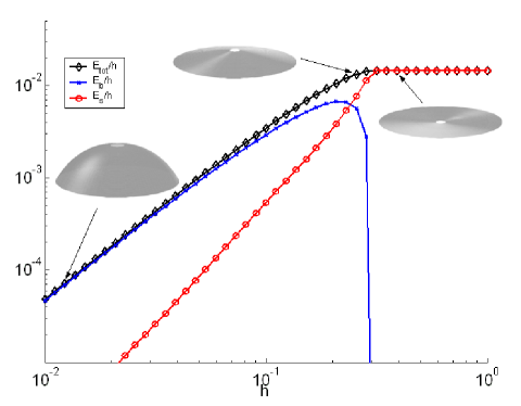
Figure 4.1: Energy scaling in positively curved discs. Total elastic energy, stretching energy and bending energy versus the thickness $h$, for non-Euclidean discs with the reference metric and lateral dimensions that are described in the text. All three energies are divided by $h$. The three rendered configurations correspond to (from right to left): a flat configuration, a weakly buckled configuration, just below the buckling threshold, and a fully buckled, almost isometric configuration (color online).

In Figure 4.1 we plot the stretching energy (red circles), the bending energy (blue crosses) and the total energy (black diamonds) versus the plate thickness $h$; all three energies were scaled by $1/h$. Except for a narrow transition region near the buckling threshold, the total energy is dominated by either the stretching energy or the bending energy. As one would expect, the bending energy drops to zero above the buckling threshold (large thickness). However, below the buckling threshold, as $h\to 0$, the stretching energy drops to zero much more rapidly than the bending energy. This last observation is in fact surprising, as naively, one would expect equilibrium to be attained when both stretching and bending energy are “equally partitioned” [33].

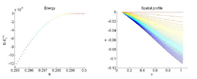
Figure 4.2: The Buckling transition. The energy variation divided by the thickness, $(E-E_{s}^{flat)})/h$ (left), and spatial profile (right) near the buckling threshold as a function of the thickness. Every profile in the right figure corresponds to an energy variation bearing the same color in the left figure. All configurations are flatter than the center disc in Figure 4.1 (note the difference in scales of the axis on the right).

In Figure 4.2 the spatial profile (a cross-section) of the elastic equilibrium configuration is shown. The transition from flat to buckled configurations occurs continuously, hence the buckled states, close to the buckling threshold, are nearly planar. This supports the validity of theories that assume small deflections from a plane (such as the FVK model) for predicting the buckling threshold. As the thickness is further reduced, the plate approaches the stress-free (isometric) configuration very fast. The assumption of small deflections from a plane fails for such configurations.

The minimal bending content, $E_{B}^{0}$, of the stretch-free configuration, and the minimal stretching content, $E_{S}^{\infty}$, of the zero bending configuration yield a crossover length scale: $h_{C}=\sqrt{E_{S}^{\infty}/E_{B}^{0}}$. Linear analysis about a flat surface gives another length scale, the buckling threshold thickness $h_{B}$. We expect the scenario depicted in Figure 4.1 to be valid for bodies in which these two length scales are relatively close. However, there are reference metrics (specifically, hyperbolic), for which all isometric immersions are convoluted, i.e. $E_{B}^{0}$ is very large. For such bodies one may obtain $h_{C}\ll h_{B}$. When this occurs, the transition region may expand. For such bodies the scaling of the elastic equilibrium energy with the thickness will be very different from the one appearing in Figure 4.1.

5 Conclusion

Natural growth of tissue as well as the plastic deformation of solids are examples of local shaping mechanisms of elastic bodies. In general, the local nature of such growth processes excludes the existence of stress-free configurations. This is the main reason why current elastic theories cannot handle properly such shaping mechanisms. In this work we derived a reduced 2D model for a class of thin plates with residual stresses, which we named “non-Euclidean plates”. Such plates are uniform across their thin dimension, but their 2D geometry is non-Euclidean. Their complicated 3D configurations cannot be obtained from existing 2D models of elasticity. Our derivation is based on a covariant formulation of 3D linear elasticity. It does not require the existence of a reference stress-free configuration, but only a 3D “reference metric” tensor, which is determined by the growth. We use this formalism together with the Kirchhoff-Love assumptions to derive a 2D energy functional. Like preceding theories, this functional decouples into bending and stretching terms. The bending term scales like the third power of the thickness and depends on surface curvature. The stretching term scales linearly with the thickness and increases with in-plane strain, which is nothing but the difference between the 2D metric tensor of a configuration and the 2D reference metric. Our theory is valid for large rotations and displacements and arbitrary intrinsic metrics.

The numerical results presented in Figure 4.1 suggest that in the general case there is no equipartition between bending and stretching energies. This in turn supports the treatment of very thin bodies as inextensible. Not only the equilibrium three-dimensional configuration is dominated by the minimization of the “small” bending energy term, but the total elastic energy is dominated by it too. The estimate of what thickness should be considered as thin involves the introduction of a new length scale $h_{C}$, which is smaller than the buckling threshold thickness. The square of this new length scale, $h_{C}^{2}$, is inversely proportional to the minimum of the Willmore functional for the prescribed $2D$ geometry. This length scale differentiates between two types of surface geometries. Surfaces which may be isometrically immersed with a moderate bending content, for which $h_{C}$ is close to the buckling threshold thickness, will follow the shaping scenario and energy profile described in Figures 4.1 and 4.2. Surfaces for which all isometric immersions have high bending contents (as is the case for some hyperbolic surfaces) may exhibit very different shaping scenarios and energetic landscapes.

The theory can be further elaborated and generalized to describe a wider range of growing bodies. We believe, however, that already in its current stage, it is a powerful tool for studying the growth of leaves and other natural slender bodies.

Acknowledgments This work was supported by the United States-–Israel Binational Foundation (grant no. 2004037) and the MechPlant project of European Union’s New and Emerging Science and Technology program. RK is grateful to M.R. Pakzad and M. Walecka for pointing out an error in the original manuscript.

Appendix A Tensors, vectors, scalars and the covariant derivative

As our treatment of elastic bodies involves the simultaneous use of two different metrics, we find it important to provide a brief summary of differential geometry in the context of the current work. In the following treatment we do not consider the most general setting but only three-dimensional manifolds immersed in $\mathbb{R}^{3}$.

Let the immersed manifold $\Omega\subset\mathbb{R}^{3}$ be the current configuration of an elastic body. A global parametrization of $\Omega$ is a one-to-one map $\boldsymbol{r}:\mathcal{D}\rightarrow\Omega$ from a domain $\mathcal{D}\subset\mathbb{R}^{3}$. Let $\boldsymbol{r}^{\prime}:\mathcal{D}^{\prime}\rightarrow\Omega$ be a different global parametrization of the current configuration. The composition $\mathbf{h}=\boldsymbol{r}^{\prime-1}\circ\boldsymbol{r}:\mathcal{D}\rightarrow\mathcal{D}^{\prime}$ is called a coordinate transformation. The coordinate transformation gradient, often denoted by $\Lambda^{j}_{i}=\partial x^{\prime j}/\partial x^{i}$, is simply the Jacobian matrix of the transformation $\mathbf{h}$, i.e. $\Lambda=\partial\mathbf{h}/\partial\mathbf{x}$. The inverse transformation gradient is $\left(\Lambda^{-1}\right)^{i}_{j}=\partial x^{i}/\partial x^{\prime j}$.

A scalar is a function $\Phi:\Omega\to\mathbb{R}$. Given a parametrization $\boldsymbol{r}:\mathcal{D}\to\Omega$, a scalar $\Phi$ induces a function $\phi:\mathcal{D}\to\mathbb{R}$ defined by $\phi(\mathbf{x})=\Phi(\boldsymbol{r}(\mathbf{x}))$. Given another parametrization $\boldsymbol{r}^{\prime}:\mathcal{D}^{\prime}\to\Omega$ with the coordinate transformation $\mathbf{h}:\mathcal{D}\to\mathcal{D}^{\prime}$, the relation between the induced functions $\phi$ and $\phi^{\prime}$ is $\phi^{\prime}(\mathbf{x}^{\prime})=\phi(\mathbf{h}^{-1}(\mathbf{x}^{\prime}))$. By a slight abuse of terminology we also call the functions $\phi$ and $\phi^{\prime}$ scalars

A vector is a function $\boldsymbol{V}$ from the manifold $\Omega$ to the local tangent space of the manifold which in our case is $\mathbb{R}^{3}$, $\boldsymbol{V}:\Omega\to\mathbb{R}^{3}$. Note that we cannot perform vector operations on pairs of vectors defined at two different points in $\Omega$, as they belong to different tangent spaces (or equivalently different copies of $\mathbb{R}^{3}$). Given a parametrization we may construct a basis $\mathbf{e}_{i}=\partial\boldsymbol{r}/\partial x^{i}$ for each tangent space. With respect to this basis we may write any vector as $\boldsymbol{V}=V^{i}\mathbf{e}_{i}$. The three functions $V^{i}:\mathcal{D}\to\mathbb{R}$ are called the contravariant components of the vector $\boldsymbol{V}$. Again by an abuse of terminology the triplet $V^{i},\,i={1,2,3}$ is called a contravariant vector. It is easy to prove that under a coordinate transformation, a contravariant vector transforms with the inverse transformation gradient, $V^{i}=\left(\Lambda^{-1}\right)^{i}_{j}V^{\prime j}$, where the left-hand side is estimated at a point $\mathbf{x}$ while the right-hand side is estimated at the corresponding point $\mathbf{x}^{\prime}=\mathbf{h}(\mathbf{x})$.

We next define the dual vector space, namely the space of covariant vectors. However, as there are many ways to define an inner product on the tangent space, there are just as many ways to define the dual vector space. The most natural inner product is the inner product induced from $\mathbb{R}^{3}$. In such a case, we define a dual base $\mathbf{e}^{j}$ by the condition $\mathbf{e}^{j}\cdot\mathbf{e}_{i}=\delta^{j}_{i}$, where $\cdot$ is the Euclidean product in $\mathbb{R}^{3}$. Any vector in the tangent space may now be decomposed with respect to this basis, $\boldsymbol{V}=V_{i}\mathbf{e}^{i}$. The triplet $V_{i}$ is called a covariant vector. Under a coordinate transformation covariant vectors transform with the transformation gradient $V_{i}=\Lambda^{j}_{i}V^{\prime}_{j}$. The inner product in the local tangent space induces an inner product on the space of contravariant vectors and the mapping of contravariant vectors to their covariant duals by

$$\boldsymbol{V}\cdot\mathbf{U}=V^{i}U^{j}\mathbf{e}_{i}\cdot\mathbf{e}_{j}=g_{ij}U^{i}V^{j}=V^{i}U_{j}\mathbf{e}_{i}\cdot\mathbf{e}^{j}=V^{i}U_{j}\delta^{j}_{i}=U_{j}V^{j},$$

where $g_{ij}=\mathbf{e}_{i}\cdot\mathbf{e}_{j}$ is called the Euclidean metric of $\Omega$ with respect to the given coordinate system. The tensor $g_{ij}$ transforms covariantly in both indices, i.e. $g_{ij}=\Lambda^{k}_{i}\Lambda^{l}_{j}g^{\prime}_{kl}$. We have identified each contravariant vector $V^{i}$ with a (covariant) vector from the dual space $V_{i}=g_{ij}V^{j}$, which is called a covariant vector. The contraction of a covariant and a contravariant vector $V^{i}U_{i}$ yields a scalar. We may choose other inner products on the space of contravariant vectors, leading to different definitions of the dual space. Let $\bar{g}_{ij}$ be a positive definite symmetric tensor, which transforms under a coordinate transformation by $\bar{g}_{ij}=\Lambda^{k}_{i}\Lambda^{l}_{j}\bar{g}^{\prime}_{kl}$ (i.e. covariantly in both indices). The operation $\langle,\rangle:\mathbb{R}^{3}\times\mathbb{R}^{3}\to\mathbb{R}$ given by $\langle\mathbf{U},\boldsymbol{V}\rangle=\bar{g}_{ij}U^{i}V^{j}$ defines an inner product on the space of contravariant vectors. For every contravariant vector there corresponds a covariant dual given by $V_{j}=\bar{g}_{ij}V^{i}$. The tensor $\bar{g}$ is called the covariant metric on $\Omega$.

Given a parameterized manifold $\boldsymbol{r}:\mathcal{D}\to\Omega$ one may easily prove that the gradient of a scalar $V_{i}=\partial_{i}\phi=\partial\phi/\partial x^{i}$ is a covariant vector. However in order to differentiate vectors we need to compare vectors that belong to different tangent spaces. To do so we use parallel transport of one of the vectors to the point where the other vector is defined. To give only a notion of what parallel transport is, we say that it will be transporting the vector along a ”straight line”, keeping a constant angle between the line and the vector. Both concepts, angles between a curve and a vector, as well as “straight lines” (geodesics), are defined by the covariant metric tensor. Thus, while the differentiation of a scalar is independent of the metric, the differentiation of a vector depends on the metric. It may be shown that the parallel transport procedure results in the following definition of the covariant derivative.

$$\bar{\nabla}_{i}V_{j}=\partial_{i}V_{j}-\bar{\Gamma}^{k}_{ij}V_{k},$$

where

$$\bar{\Gamma}^{i}_{jk}={\textstyle\frac{1}{2}}\bar{g}^{il}(\partial_{j}\bar{g}_{kl}+\partial_{k}\bar{g}_{jl}-\partial_{l}\bar{g}_{jk}).$$

One may verify that $\bar{\nabla}_{i}V_{j}$ transforms covariantly in both indices under a coordinate transformation. The covariant differentiation of a contravariant vector is given by

$$\bar{\nabla}_{i}V^{j}=\partial_{i}V^{j}+\bar{\Gamma}^{j}_{ik}V^{k}.$$

Note that $\bar{\Gamma}^{i}_{jk}$ is not covariant or contravariant in any of its components. Henceforth, we will use the term tensors to refer to multidimensional arrays for which all indices transform covariantly or contravariantly, thus $\bar{\Gamma}$ is not a tensor. One may easily verify that the multiplication or contraction of tensors results in a tensor. The differentiation of a tensor should be treated as if the tensor is an external product of vectors and apply the covariant derivative through the Leibnitz product rule. For example in the two-dimensional case we have

$$\bar{\nabla}_{k}M_{ij}=\partial_{k}M_{ij}-\bar{\Gamma}^{l}_{kj}M_{il}-\bar{\Gamma}^{l}_{ki}M_{jl}.$$

In general, when working with explicit parameterizations we need, in order to prove that a certain parameter is a tensor (e.g. a scalar or a covariant vector), to prescribe it for all possible parameterizations, and show that it obeys the correct transformation rules. This is the case for the current metric $g_{ij}=\partial_{i}\boldsymbol{r}\cdot\partial_{j}\boldsymbol{r}$. It is defined for all possible parameterizations and obeys the covariant transformation rules. As the reference metric coincides with the current metric (for a local stress-free configuration), we have that $\bar{g}$ is also a rank-two covariant tensor. However some quantities are tensorial by definition, for example $S^{ij}=dw/d\varepsilon_{ij}$, which is the derivative of a scalar with respect to a covariant tensor. For such quantities we may determine their value for one (convenient) parametrization, and obtain their value for all other parameterizations through the tensorial transformation rule. This is the case for the elastic tensor $A^{ijkl}$, as may be observed in (2.4).

References

- [1] A.E.H. Love. The mathematical theory of elasticity. Cambridge University Press, 1906.
- [2] W.T. Koiter. On the nonlinear theory of thin elastic shells. Proc. Kon. Ned. Acad. Wetensch., B69:1–54, 1966.
- [3] W.T. Koiter. Comment on: The linear and non-linear equilibrium equations for thin elastic shells according to the Kirchhoff-Love hypotheses. Int. J. mech. Sci., 12:663-664, 1970.
- [4] P.G. Ciarlet. Mathematical elasticity, volume 2. North-Holland, Amsterdam, 1997.
- [5] G. Friesecke, R.D. James, and S. Müller. A hierarchy of plate models derived from nonlinear elasticity by Gamma-convergence. Arch. Rat. Mech. Anal., 180:183–236, 2006.
- [6] E. Sharon, M. Marder and H.L. Swinney. Leaves, flowers and garbage bags: Making waves American Scientist., 92:254-261, 2004.
- [7] A. Goriely and M. Ben-Amar. On the definition and modeling of incremental, cummulative, and continuous growth laws in morphoelasticity Biomechan. Model Mechanobiol., 6:289296, 2007.
- [8] M. Ben Amar and A. Goriely. Growth and instabilities in elastic tissues. J. Mech. Phys. Solids, 53:2284–2319, 2005.
- [9] A. Hoger. Residual stress in an elastic body: a theory for small strains and arbitrary rotation. Journal of Elasticity., 31:1–24, 1993.
- [10] M. Marder and N. Papanicolaou. Geometry and elasticity of strips and flowers. Journal of Statistical Physics., 125:1609-1096, 2006.
- [11] B. Audoly and A. Boudaoud. Self-similar structures near boundaries in strained systems. Phys. Rev. Lett., 91:086105, 2003.
- [12] J. Huang, M. Juszkiewicz, W.H. de Jeu, E. Cerda, T. Emrick, and N. Menon. Capillary wrinkling of floating thin polymer films. Science, 317:650–653, 2007.
- [13] K. Efimenko, M. Rackaitis, E. Manias, A. Vaziri, L. Mahadevan and J. Genzer. Nested self-similar wrinkling patterns in skins. Nat. Mat., 4:293–297, 2005.
- [14] D. P. Holmes and A. J. Crosby Snapping surfaces. Adv. Mater. 19:3589-3593, 2007.
- [15] Soft matter gets smart. Materials Today, 10:4, 2007.
- [16] Y. Forterre, J.M. Skotheim, J. Dumais, and L. Mahadevan. How the Venus flytrap snaps. Nature, 433:421–425, 2005.
- [17] J.S. Park, J. S .F. Chu, C. Cheng, F. Chen, D. Chen and S. Li. Differential effects of equiaxial and uniaxial strain on mesenchymal stem cells. Biotechnology and Bioengineering., 88:359-368, 2004.
- [18] E. Cerda and L. Mahadevan. Geometry and physics of wrinkling. Phys. Rev. Lett., 90:074302–1, 2003.
- [19] F. Sidoroff and A. Dogui. Thermodynamics and duality in finite elastoplasticity Continuum Thermomechanics, 389-400, 2002.
- [20] F. Sidoroff. Incremental constitutive equation for large strain elasto plasticity. International Journal of Engineering Science, 20:1:19-26, 1982.
- [21] A. E. Green and P. M. Naghdi. Some remarks on elastic-plastic deformation at finite strain International Journal of Engineering Science, 9:12:1219-1229, 1971.
- [22] E. Sharon, B. Roman, M. Marder, G.S. Shin, and H.L. Swinney. Mechanics: Buckling cascades in free sheets. Nature, 419:579–580, 2002.
- [23] Y. Klein, E. Efrati, and E. Sharon. Shaping of elastic sheets by prescription of Non-Euclidean metrics. Science, 315:1116 – 1120, 2007.
- [24] T. Mora and A. Boudaoud Buckling of swelling gels The European Physical Journal E - Soft Matter 20:2:119-124, 2006
- [25] P.G. Ciarlet. An introduction to differential geometry with applications to elasticity. Springer, Dordrecht, The Netherlands, 2005.
- [26] C. Truesdell. The mechanical foundations of elasticity and fluid dynamics Indiana Univ. Math. J., 1:125–300, 1952.
- [27] F. John. Estimates for the derivatives of the stresses in thin shell and interior shell equation. Comm. Pure and Appl. Math., 18:235–267, 1965.
- [28] T.J. Willmore. Reimannian geometry. Oxford University Press, Oxford, 1993.
- [29] R. A. Adams. Sobolev spaces. Academic Press, London, 1975.
- [30] G. Dal Maso. An Introduction to -Converegence. Birkhäuser, Boston, 1993.
- [31] D.J. Steigmann. Tension-field theory. Proc. Roy. Soc. London Sect. A, 429:171–143, 1990.
- [32] P.G. Ciarlet. The continuity of a surface as a function of its two fundamental forms. J. Math. Pures Appl., 82:253–274, 2003.
- [33] S.C. Venkataramani. Lower bounds for the energy in a crumpled elastic sheet - a minimal ridge. Nonlinearity, 17:301–312, 2004.
- [34] J.H.C. Wang and B.P. Thampatty. An introductory review of cell mechanobiology Biomechan. Model Mechanobiol., 5:116, 2006.