DETECTION OF CHROMATIC MICROLENSING IN Q 2237+0305 A

Abstract

We present narrowband images of the gravitational lens system Q 2237+0305 made with the Nordic Optical Telescope in eight different filters covering the wavelength interval 3510-8130 Å. Using point-spread function photometry fitting we have derived the difference in magnitude versus wavelength between the four images of Q 2237+0305. At $\lambda=4110$ Å, the wavelength range covered by the Strömgren-v filter coincides with the position and width of the CIV emission line. This allows us to determine the existence of microlensing in the continuum and not in the emission lines for two images of the quasar. Moreover, the brightness of image A shows a significant variation with wavelength which can only be explained as consequence of chromatic microlensing. To perform a complete analysis of this chromatic event our observations were used together with Optical Gravitational Lensing Experiment light curves. Both data sets cannot be reproduced by the simple phenomenology described under the caustic crossing approximation; using more realistic representations of microlensing at high optical depth, we found solutions consistent with simple thin disk models ($r_{s}\varpropto\lambda^{4/3}$); however, other accretion disk size-wavelength relationships also lead to good solutions. New chromatic events from the ongoing narrow band photometric monitoring of Q 2237+0305 are needed to accurately constrain the physical properties of the accretion disk for this system.

1. Introduction

Gravitational lensing is independent of wavelength (Schneider, Ehlers & Falco 1992). However, in many gravitationally lensed quasars, differences in color between the images are observed. These chromatic variations could be produced by two effects: differential extinction in the lens galaxy and chromatic microlensing. When each image’s light crosses the interstellar medium of the lens galaxy it may be affected in different amounts by patchily distributed dust. This results in differential extinction between pairs of images, and makes possible the determination of the extinction law of the lens galaxy (Nadeau et al. 1991; Falco et al. 1999; Motta et al. 2002; Muñoz et al. 2004; Mediavilla et al. 2005; Elíasdóttir et al. 2006). The other chromatic phenomenon arises when stars or compact objects in the lens galaxy are nearly aligned with the line of sight between the quasar image and the observer. Due to the relative motion between the quasar, the lens and the observer, the quasar image undergoes a magnification or demagnification known as microlensing (Schneider, Kochanek $\&$ Wambsganss 2006 and references therein). Therefore, fluctuations in the brightness of a quasar image will be a combination of the intrinsic quasar variability and the microlensing from the stars or compact objects in the lens galaxy. The intrinsic variability of the lensed quasar will appear in all images with certain time delay due to the different light travel times. Once this delay is determined, the light curves of the different images can be shifted, and then subtracted. The remaining fluctuations can be assumed to be caused only by microlensing. The microlensing magnification depends on the angular size of the source, in this case on the accretion disk of the quasar. Because the accretion disk is hotter closer to the black hole, and because the emission of the accretion disk depends on temperature, different magnifications may be observed at different wavelengths. This effect is known as chromatic microlensing, and it offers unprecedented perspectives into the physical properties of accretion disks (Wambsganss $\&$ Paczynski 1991). Its detection in a lens system will lead to accurate constraints in the size-wavelength scaling.

Different authors have made some attempts to detect chromatic microlensing and use it with different scopes. However, in many cases the detection of chromatic microlensing was rather ambiguous, since in general it is not easy to disentangle this effect from others with similar observational signatures (Wisotzki et al. 1993; Nadeau et al. 1999; Wucknitz et al. 2003; Nakos et al. 2005). The first significant applications of chromatic microlensing appeared in a very recent work of Poindexter et al. (2008). They have used chromatic microlensing in order to determine the size of the accretion disk of HE 1104-1805 as well as its size-wavelength scaling. More recently, Anguita et al. (2008) have also made these kinds of studies in Q 2237+0305. In both cases they found solutions consistent with the simple thin disk model (Shakura $\&$ Sunyaev 1973), but stronger constraints would be needed to accurately determine the size of the accretion disk.

In this work, we present a chromatic microlensing detection in one of the images of Q 2237+0305 (Huchra et al. 1985). This lens system has very good properties to study microlensing events. The light coming from a distant quasar at $z_{S}=1.695$ is deflected by a nearby spiral galaxy ($z_{L}=0.039$) forming four quasar images nearly symmetrically distributed around the lens center. Since the light passes through the central part of the galaxy, where the microlensing optical depth is very large, high magnification events (HMEs) occur very frequently. Moreover, since the galaxy has a very low redshift, and due to the symmetry in the positions of the images, time delays are expected to be very small ($<1$ day; Vakulik et al. 2006; Koptelova et al. 2006). Therefore, time delay corrections are not needed to study microlensing in this lens system, and the flux ratio between the images will remove the contribution of the intrinsic quasar variability in the light curves.

Specifically, we analyze a particular chromatic microlensing event, and study the physical scenarios in which this effect can be produced. The results obtained in this work are the first step toward obtaining precise constraints in the physical properties of the quasar accretion disk. In §2 the observations and the data analysis are presented. The data fitting techniques and different models to describe the observed chromatic microlensing are discussed in §3. A summary of the main conclusions appears in §4.

2. Observations and Data analysis

On the nights of August 26 and 28 2003, we observed Q 2237+0305 with the 2.56 m Nordic Optical Telescope (NOT) located at the Roque de los Muchachos Observatory, La Palma (Spain), using the 2048$\times$2048 ALSFOC detector. Its spatial scale is 0.188 arsec/pixel. Seven narrow filters plus the wide I-Bessel were used. The whole set covered the wavelength interval 3510-8130 Å. Table 1 shows a log of our observations.

Table 1Log of ALSFOC Observations

Target	Observation Date	Filter	Exposure (s)
Q 2237+0305	2003 Aug 26	Str-u ($\lambda=3510$ Å)	$4\times 600$
Q 2237+0305	2003 Aug 26	Str-v ($\lambda=4110$ Å)	$3\times 600$
Q 2237+0305	2003 Aug 26	Str-b ($\lambda=4670$ Å)	$3\times 600$
Q 2237+0305	2003 Aug 26	Str-y ($\lambda=5470$ Å)	$3\times 600$
Q 2237+0305	2003 Aug 26	Iac#28 ($\lambda=6062$ Å)	$3\times 600$
Q 2237+0305	2003 Aug 26	H$\alpha$ ($\lambda=6567$ Å)	$3\times 600$
Q 2237+0305	2003 Aug 26	Iac#29 ($\lambda=7015$ Å)	$3\times 600$
Q 2237+0305	2003 Aug 26	I-band ($\lambda=8130$ Å)	$4\times 100$
Q 2237+0305	2003 Aug 28	Str-u ($\lambda=3510$ Å)	$3\times 600$
			$2\times 900$
Q 2237+0305	2003 Aug 28	Str-v ($\lambda=4110$ Å)	$3\times 600$
Q 2237+0305	2003 Aug 28	Str-b ($\lambda=4670$ Å)	$3\times 420$
Q 2237+0305	2003 Aug 28	Str-y ($\lambda=5470$ Å)	$3\times 420$
Q 2237+0305	2003 Aug 28	Iac#28 ($\lambda=6062$ Å)	$3\times 420$
Q 2237+0305	2003 Aug 28	H$\alpha$ ($\lambda=6567$ Å)	$3\times 420$
Q 2237+0305	2003 Aug 28	Iac#29 ($\lambda=7015$ Å)	$3\times 420$
Q 2237+0305	2003 Aug 28	I-band ($\lambda=8130$ Å)	$3\times 100$

Among the filters that we used only two were affected by the emission lines of the quasar. The Strömgren-u filter was affected by almost 40% by the Ly$\alpha$ emission line, where the emission lines of the quasar and its nearby continuum were modeled according to the SDSS quasar composite spectrum (Vanden Berk et al. 2001) to perform this estimation. At $\lambda=4110$Å the wavelength range covered by the Strömgren-v filter coincides with the position and width of the CIV emission line.

The data were reduced using standard procedures with IRAF packages, and PSF photometry fitting was used to derive the difference in magnitude versus wavelength between the four images of Q 2237+0305. The galaxy bulge was modeled with a de Vaucouleurs profile, and the quasar images as point sources. This model was convolved with different PSFs observed simultaneously with the lens system in each of the frames, and compared to the image through $\chi^{2}$ statistics ( McLeod et al. 1998; Lehár et al. 2000). Due to the good seeing conditions (0”.6 in I band), the results of the photometry were excellent even in the bluest filters.

Table 2 presents the measurements of the differences in magnitude in each filter. In Figure 1, we have plotted six magnitude differences versus wavelength (three of which are independent) between the four images of the quasar.

Figure 1.— Magnitude differences as a function of the observed wavelength for Q 2237+0305 (NOT data). Images A and C show a clear signature of microlensing in the continuum but not in the emission lines. Moreover, the chromatic variation observed in image A could only be explained as a consequence of chromatic microlensing. The wavelength widths covered by the emission lines that affect two of our filters (CIV and Ly$\alpha$) are indicated.

Table 2Q 2237+0305 PHOTOMETRY

Filter	$m_{B}-m_{A}$	$m_{C}-m_{A}$	$m_{D}-m_{A}$
Str-u ($\lambda=3510$ Å)	1.57$\pm$0.06	1.57$\pm$0.06	1.52$\pm$0.06
Str-v ($\lambda=4110$ Å)	1.41$\pm$0.02	1.45$\pm$0.04	1.39$\pm$0.02
Str-b ($\lambda=4670$ Å)	1.67$\pm$0.03	1.47$\pm$0.04	1.59$\pm$0.04
Str-y ($\lambda=5470$ Å)	1.65$\pm$0.02	1.45$\pm$0.06	1.58$\pm$0.03
Iac#28 ($\lambda=6062$ Å)	1.58$\pm$0.03	1.39$\pm$0.04	1.52$\pm$0.04
H$\alpha$ ($\lambda=6567$ Å)	1.46$\pm$0.02	1.32$\pm$0.03	1.46$\pm$0.05
Iac#29 ($\lambda=7015$ Å)	1.56$\pm$0.03	1.38$\pm$0.02	1.52$\pm$0.02
I-band ($\lambda=8130$ Å)	1.40$\pm$0.03	1.22$\pm$0.02	1.38$\pm$0.04

Figure 2.— Magnitude differences between Q 2237+0305 images obtained from OGLE V-band light curves. The dashed line indicates our observation date, and the solid lines limit the selected time interval in which the study was performed.

The difference in magnitude between B and D does not show any chromatic variation, and it is reasonable to suppose that neither B nor D is undergoing flux variations with wavelength. The differences $m_{B}-m_{C}$, and $m_{D}-m_{C}$, show that both curves have the same trend, and this implies that the magnitude of image C varies with wavelength (consistent with our hypothesis that neither image B nor D suffers of chromaticity). In these curves it is also observed that there is no magnitude variation with the wavelength in the region between 4670 Å and 8130 Å, but at the wavelengths corresponding to the Strömgren-v and Strömgren-u filters, which are the only ones affected by emission lines, we observed a deviation from the trend. As we stated above the Strömgren-u filter was affected by almost 40% by the Ly$\alpha$ emission line, and at $\lambda=4110$ Å, the wavelength range covered by the Strömgren-v filter coincides with the position and width of the CIV emission line. Then, the dependence of $m_{B}-m_{C}$ or $m_{D}-m_{C}$ with wavelength observed under our filter set configuration is the observational signature expected for image C being affected by microlensing in the continuum but not in the emission lines. The fact that microlensing is absent in the emission lines confirms the relatively large size of the broad-line region (BLR) in Q 2237+0305 according to the existing relation between the size of the BLR and the intrinsic luminosity of the quasar (Kaspi et al. 2000, Abajas et al. 2002).

Finally, we analyzed the differences between image A and the other ones. Again, as the trend of the curves is the same for each difference, we conclude that A is the image which undergoes flux variations. As the points corresponding to Strömgren-v and Strömgren-u filters deviate from the respective trend, we can conclude again that image A is undergoing microlensing in the continuum but not in the emission lines. An even more interesting result appears from analyzing the points corresponding to the continuum, where image A shows a significant variation with wavelength. In principle, this effect could be produced by extinction and/or chromatic microlensing. But as image A is the one undergoing the flux variation, if it were due to extinction the slope of the curve should be negative, and not positive as it is observed in the plot. Therefore, we have strong evidence of chromatic microlensing in image A.

Since we have observations of only two consecutive nights in that period, to know what was the signature of the microlensing in the system, we used the public Optical Gravitational Lensing Experiment(OGLE) data (Woźniak et al. 2000). Since 1999 January OGLE has been monitoring Q 2237+0305 in the V-band. In Figure 2, three independent magnitude differences between the quasar images obtained from their data are plotted. In the time interval between HJD 2452764 and HJD 2453145 (indicated in Figure 2 between solid lines) the differences ($m_{B}-m_{C}$) and ($m_{B}-m_{D}$) are almost constant. This would imply that the flux variations of the images B, C, and D are caused mainly by intrinsic variability of the quasar, which agrees with our previous hypothesis that neither B, C nor D is undergoing chromaticity originated by an HME. The fact that in our observations we have detected (nonchromatic) microlensing in image C is also in agreement with OGLE data, since a constant micro-magnification value during this period justifies both observations. Therefore, the brightness fluctuations ($\sim 0.3$ mag) observed in the difference ($m_{B}-m_{A}$) can be assumed to be due only to microlensing-induced variability in image A. In other words, from Figure 2 we can say that image A was in fact undergoing an HME on the dates of our observations which correspond to HJD 2452878.5 and 2452880.5.

Summarizing we can say that, based on the 2003 NOT observations, images C and A are undergoing microlensing in the continuum but not in the emission lines, and that image A is also affected by chromatic microlensing. In the next section this unambiguous detection of chromatic microlensing is used, along with the OGLE data from HJD 2452764 to HJD 2453145, to explore the phenomenology of the detected microlensing event and to study the physical properties of the accretion disk.

3. Data fitting

3.1. Chromatic microlensing and caustic crossing approximation

Figure 3.— Typical observable effects of chromatic microlensing. The amplitude of the microlensing is different at different wavelengths due to the expected dependence of the accretion disk size with wavelength. In addition, the maximum magnification is reached at a different instant with a time delay $\Delta t_{max}$ (see the text).

To review some basic aspects of chromatic microlensing we will start recalling the simplest model for microlensing, the caustic crossing approximation. Taking a Cartesian coordinate frame in which the caustic lies along the $y$-axis, the magnification at a distance $x$ is proportional to the well-known expression $1+\beta\ H(x)/\sqrt{x}$  (Schneider $\&$ Weiss 1987). Here $H$ represents the Heaviside step function, and $\beta$ measures the caustic strength. Assume a brightness profile for the quasar accretion disk given by

$$I(r)=\frac{I_{0}}{2\pi r_{s}^{2}}\Psi(r/r_{s}),$$ (1)

where $r_{s}$ represents a typical size scale of the quasar accretion disk; provided a global factor (or a global constant in magnitudes) containing the magnification background, the magnification of the quasar accretion disk is

$$\mu\sim 1+\frac{\beta}{\sqrt{r_{s}}}\ \phi(\xi),$$ (2)

where $\xi\equiv\frac{x_{0}}{r_{s}}$ is the distance between the center of the disk and the caustic, $x_{0}$, in units of the scale radius $r_{s}$, and it can take negative or positive values to distinguish both sides of the caustic. Analytical expressions can be straightforwardly obtained for several accretion disk models, e.g., Gaussian (Schneider $\&$ Weiss 1987) or power laws (Shalyapin 2001). If a constant relative source plane velocity is considered between the disk and the caustic, then $x_{0}=v\ (t-t_{0})$, where $t_{0}$ is the instant of time at which the center of the disk is located at the caustic position. Therefore we can see that an HME due to a single caustic crossing is, in addition to the crossing time $t_{0}$, a function of only two parameters: $\beta^{\prime}\equiv\beta/\sqrt{r_{s}}$ and $r^{\prime}_{s}\equiv r_{s}/v$. Due to this degeneracy, the disk size $r_{s}$ and the velocity $v$ cannot be determined independently but only the ratio $r_{s}/v$.

Figure 3 shows the typical observable effects of chromatic microlensing. Because the size of the accretion disk is expected to change with wavelength, the amplitudes of the HME events observed at different wavelengths are different. The maximum magnification, in magnitudes, relative to the local average microlensing magnification background (see Figure 3) will be

$$\Delta m_{max}=-2.5\ \mathrm{Log}\left[1+\frac{\beta}{\sqrt{r_{s}}}\ \phi(\xi_{max})\right].$$ (3)

The value of $\phi(\xi_{max})$ depends on the brightness profile model. For instance, for a Gaussian model $\phi(\xi_{max}\simeq 0.765)\simeq 1.021$. Hence, given a brightness profile model, the observable $\Delta m_{max}$ provides a direct estimation of the dimensionless parameter $\beta/\sqrt{r_{s}}$.

If an HME is monitored at two different wavelengths, then using equation (3) the ratio between the different corresponding sizes is

$$\frac{r^{1}_{s}}{r^{2}_{s}}=\left[\frac{10^{-\Delta m^{2}_{max}/2.5}-1}{10^{-\Delta m^{1}_{max}/2.5}-1}\right]^{2}$$ (4)

and it is very remarkable that, provided that equation (2) is satisfied, this expression is independent of the brightness profile of the accretion disk. As an example we can use the recent results obtained by Anguita et al. (2008), where they analyzed another HME observed in the 1999 OGLE campaign. From Figure 2 in their paper it is possible to estimate that $\Delta m^{g}_{max}\sim-0.8$ (see also OGLE ${}^{\ref{oglelink}}$ data for a better sampling) and $\Delta m^{r}_{max}\sim-0.57$. Therefore, applying equation (4) $r^{r}_{s}/r^{g}_{s}\sim 2.5$. This value is slightly different from the ratio obtained in their paper where they use a magnification pattern instead of a caustic crossing.

Figure 4.— OGLE V-band ($m_{B}-m_{A}$) data. The best fit using a simple double-caustic crossing approximation and a Gaussian brightness profile is shown. The dashed line indicates our observation date.

Another interesting property is obtained with the observable $\Delta t_{max}$, i.e., the difference in time to reach the maximum magnification for each source size (see Figure 3). It is straightforward to obtain

$$\Delta t_{max}=\xi_{max}\ r^{\prime 1}_{s}\left[1-\frac{r^{2}_{s}}{r^{1}_{s}}\right].$$ (5)

Although it depends on the quasar disk model, it allows us to determine directly the size-velocity ratio. Unfortunately the light curve shown in Figure 2 of Anguita et al. (2008) has not the temporal sampling to accurately estimate $\Delta t_{max}$, but assuming a value $\sim 10$ days we would find the order of magnitude for $r^{\prime g}_{s}\equiv r^{g}_{s}/v\sim 20$ day^-1.

3.2. Double-caustic crossing approximation

We start using the simple model of the caustic crossing approximation with the aim of finding a simultaneous fit of the difference $(m_{B}-m_{A})$ obtained from the OGLE V-band light curves (over the temporal range from HJD 2452764 to HJD 2453145) (Figure 4) and our chromatic observation. As explained before, in this case, the fluctuations in $(m_{B}-m_{A})$ correspond only to microlensing-induced variability in image A. Because of the shape of the data we assumed that the image A of the quasar is undergoing a double-caustic crossing event, and we considered a Gaussian brightness profile for the accretion disk $I(r)=\frac{I_{0}}{2\pi r_{s}^{2}}\exp\left[-r^{2}/2r^{2}_{s}\right]$. The main parameters involved in our fitting are: the ratio between $r_{s}$ and the relative caustic-disk source plane velocity, $r_{s}^{\prime}=r_{s}/v$, the dimensionless caustic stretch divided by $\sqrt{r_{s}}$, $\beta_{i=1,2}^{\prime}$, the time corresponding to each caustic crossing, $t_{i=1,2}$, and the relative microlensing magnification background between each side of the caustics, where the subindex $i=1,2$ refers to each of the caustics.

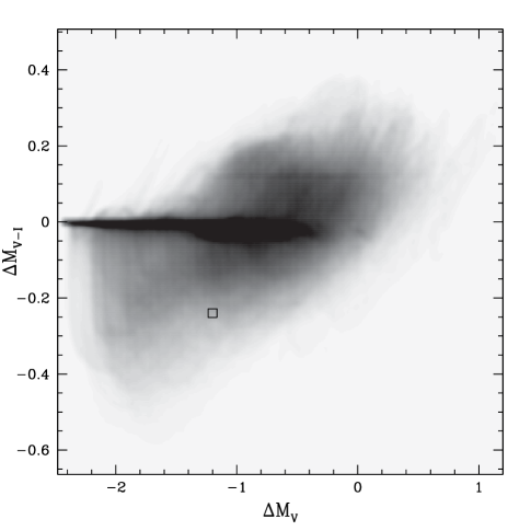
Figure 5.— Image A “chromatic map”. $\Delta M_{V}$ represents the microlensing magnification in the V-band, and $\Delta M_{V-I}$ is the difference in magnitude $m_{V}-m_{I}$ due to chromatic microlensing. The open square corresponds to the observed values. The different grayscales in the map correspond to different values of the probability of occurrence.

The estimation of the model parameters was carried out with a $\chi^{2}$ minimization fitting method. Due to the scatter of the OGLE data, the points were binned to have only one point per day, which value corresponds to the averaged binned points, and which associated error corresponds to the dispersion calculated in each day. Because the first caustic crossing event is not completely sampled, the parameters associated with it cannot be determined; however the ones associated with the second caustic can be bounded ($\beta_{2}=0.3\pm 0.1$, $t_{2}=3008\pm 12$). Figure 4 shows the best fit that corresponds to $\chi^{2}/N_{f}=0.22$, where $N_{f}$ is the number of degrees of freedom.

Although this simple model produces a good light curve fitting for the OGLE data, it cannot reproduce the observed chromatic effect. Taking as reference the filters Strömgren-y and I-band, we observe a chromaticity $(m^{V}_{A}-m^{I}_{A})=-0.24\pm 0.05$ mag . However, assuming a radius-wavelength scaling that goes as $r_{s}\varpropto\lambda^{4/3}$ (thin-disk model), the chromaticity that can be produced by this double-caustic approximation model on the day of our observation (HJD 2452879.5) is $\sim-0.01$ mag, and a maximum chromaticity of $\sim-0.25$ mag is only achieved for an unrealistic ratio $r^{I}_{s}/r^{V}_{s}\gtrsim 10^{2}$. The limitation of the caustic crossing approximation in reproducing the observed chromatic microlensing magnification is due to the fact that the induced chromaticity is only a function of the caustic stretch $\beta/\sqrt{r_{s}}$, and it is independent of the microamplification background. However, as we will see in the next subsection, this is not the case in a more realistic scenario.

This is a good example which confirms, as stated by Kochanek (2004), that due to the high microlensing optical depth of Q 2237+0305 it is unlikely that the system undergoes a “clean” caustic crossing. In this sense the model that we used here is too simple to approach the real behavior of the system. The appropriate way to find a solution is to consider a more realistic physical scenario, i.e., a magnification pattern is needed to describe the observational signatures in this case.

3.3. Modeling microlensing from magnification maps

Magnification maps for images A and B would be needed to find trajectories that reproduce ($m_{B}-m_{A}$) V-band OGLE difference during the period of interest. As stated before, in the time interval between HJD 2452764 and HJD 2453145, the brightness fluctuations observed in $(m_{B}-m_{A})$ are due only to microlensing in image A, since image B is mainly affected by intrinsic variability of the quasar. Therefore, the behavior of image B can be represented with a constant magnification value, and magnification patterns for this image are not needed. Its contribution to the $(m_{B}-m_{A})$ magnitude difference, as well as any extinction correction or uncertainties in the macromodels will be included in a constant parameter, $m_{0}$, that will shift image A microlensing fluctuations.

We have built magnification patterns for image A using the inverse ray shooting technique (Wambsganss 1990, 1999) and the inverse polygon mapping (Mediavilla et al. 2006). It was assumed that all the mass responsible for microlensing is in compact objects of 1 $M_{\odot}$, and the values for the convergence of $\kappa=0.36$ and for the shear of $\gamma=0.4$ (Schmidt et al. 1998) were considered. The map dimensions are of $4096\times 4096$ pixels which correspond to physical dimensions of $20\ r_{E}\times 20\ r_{E}$. Therefore the magnification pattern has a resolution of $0.005$ $r_{E}/$pixel.

Figure 6.— Histogram of the number of tracks, $N_{T}$, that reproduce OGLE V-band data as well as the chromatic data set, as a function of the magnification ratio between images A and B, $m_{0}$.

With the aim of evaluating the likelihood of reproducing the microlensing and chromatic microlensing magnifications we observed, a “chromatic map” for image A was built (Figure 5). To each point in the map with coordinates ($\Delta M_{V}$, $\Delta M_{V-I}$), corresponds a value of the probability of occurrence. Here $\Delta M_{V}\equiv-2.5\log\mu_{V}$ represents the microlensing magnification in V-band, and $\Delta M_{V-I}$ is the difference in magnitude $m_{V}-m_{I}$ due to the disk size-wavelength dependence (i.e. chromatic microlensing). To compute those magnitude differences, since we are considering an extended object, the pattern was convolved with the brightness distribution of the source and, as before, we assumed a Gaussian profile. At $\lambda=5430$ Å (V-band) a Gaussian width of $r_{s}=0.03\ r_{E}$ ($\sim 1.5$ light days) was adopted which corresponds to the average value found by Kochanek (2004). At $\lambda=8130$ Å (I-band), assuming that the accretion disk has a size-wavelength dependence that goes as $r_{s}\varpropto\lambda^{4/3}$ (thin-disk model), the pattern was convolved with a Gaussian width of $r_{s}=0.05\ r_{E}$ ($\sim 3$ light days).

Once the quantities $\Delta M_{V}$ and $\Delta M_{V-I}$ were evaluated at each pixel in the V-band convolved pattern and in the V-I difference pattern respectively, the probability of occurrence was calculated, and its distribution is represented in Figure 5.

Figure 7.— In the top panel, the best OGLE light curve fitting (dashed line; $\chi^{2}=10$) is shown together with the fitting that also reproduces the chromaticity ($\chi^{2}=13$; solid line). In the lower panel the chromatic effects produced along each trajectory are compared, where the filled square represents the observed chromaticity.

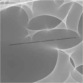
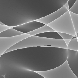
Figure 8.— Left: Trajectory that best fits the OGLE data, but which does not reproduce the observed chromaticity. Right: Trajectory that best reproduces both data sets. Both sections of the magnification pattern have a physical size of $2.9\ r_{E}\times 2.9\ r_{E}$.

As far as the baseline for no microlensing (i.e., the magnification ratio between the images in the absence of microlensing) is unknown; the true value of $\Delta M_{V}$ is unknown. However, our observations in the filters Str-u and Str-v which are affected by the emission lines would allow us, in principle, to estimate separately the true magnification ratio between the images, and the microlensing. This is because the observed flux for the image $i$ is given by $F_{i}=\mu^{macro}_{i}(\mu^{micro}_{i}F_{c}+F_{l})$, where the subindex $c$ refers to the continuum and $l$ to the emission lines, i.e., the microlensing is affecting the continuum but not the emission lines. In practice this calculation is complicated to do because a model for the continuum and the emission lines have to be assumed, and also because small variations in the measured magnitudes introduce large uncertainties in both factors ($\mu^{macro}_{i}$ and $\mu^{micro}_{i}$). For instance, these large uncertainties do not allow the determination of the microlensing in image C. For image A, using our measurement in the Str-u filter and modeling the Ly${\alpha}$ emission line and its nearby continuum according to the SDSS quasar composite spectrum (Vanden Berk et al. 2001), we estimate a flux ratio $F_{B}/F_{A}\sim F_{D}/F_{A}\sim 0.6\pm 0.2$ and a microlensing magnification of $\mu_{V}\sim-1.2\pm 0.4$ mag. These flux ratios are in agreement with those found by Wayth et al. (2005). Moreover a similar macroamplification for the four images would be a reasonable scenario for a macrolens model describing the large symmetry observed in the four image positions, but it would imply that the anomalous brightness of the image A is produced by a large microamplification background.

We found that given a microlensing magnification of $\mu_{V}=-1.2\pm 0.4$ mag for image A, the probability of observing a chromatic microlensing magnification $m^{V}_{A}-m^{I}_{A}=-0.24\pm 0.05$ mag is of $\sim 4\%$. Even though this value is not very high, the probability of finding a solution is now different from zero. That is, the modeling of microlensing chromaticity from microlensing magnification maps leads to a phenomenology (richer than that associated with the caustic crossing approximation) that includes the observed data. The square in the “chromatic map”(Figure 5) corresponds to these values. The probability increases if, instead of using the $r_{s}\varpropto\lambda^{4/3}$ law, greater values of $r^{I}_{s}/r^{V}_{s}$ are considered, reaching a maximum value of $\simeq 27\%$ for $r^{I}_{s}/r^{V}_{s}\simeq 3.9$.

The microamplification estimation of $\mu_{V}=-1.2\pm 0.4$ mag could be affected by large uncertainties; for instance a real source spectrum with deviations from the Gaussian approximation of the emission line profile (Vanden Berk al. 2001), or dust in the lens galaxy, would lead to different flux ratios between the images and microamplification values, and therefore it must be only considered as a tentative estimation. A spectroscopic monitoring of the system would be needed to clarify the true magnification ratios and microlensing for the images.

To complete our study we explore the possibilities of jointly reproducing the $m_{B}-m_{A}$ V-band OGLE data and our observations. In the first place, we fit the OGLE data using the V-band convolved pattern, where $2\times 10^{6}$ random trajectories were traced, and compared with the OGLE difference $m_{B}-m_{A}$ through a $\chi^{2}$ statistics. The source plane velocity, and the macromagnified image difference were varied in the ranges 0.0015$\ r_{E}$ HJD${}^{-1}<v<0.0065\ r_{E}$ HJD^-1, and -1.08 mag $<m_{0}<$ 2.59 mag respectively. The wide range of the covered source plane velocities includes already existing limits (Kochanek 2004), and the bounds set for the macromagnified image difference were chosen according to covering a large range of microlensing magnifications (from $-2.48$ mag to $1.19$ mag ). From a total of $7.16\times 10^{10}$ simulated trajectories we have found $2711,493$ tracks with $\chi^{2}/N_{f}<1$ (where $N_{f}=57$) which satisfactorily fit the OGLE data.

The next step is to determine in how many of those tracks the observed chromaticity ($m^{V}_{A}-m^{I}_{A}=-0.245\pm 0.05$) is reproduced. We found that 6443 of the tracks which reproduce OGLE data also reproduce, at the $1-\sigma$ level, our chromatic observation. The probability distribution of $m_{0}$ considering those trajectories is bimodal (Figure 6), with peaks located at $m_{0}\sim 0.1$ and $m_{0}\sim 0.9$, which corresponds to microlensing magnification values of $\mu_{V}\sim-1.4$ and $\mu_{V}\sim-0.6$ respectively. Solutions are found in all the velocity range selected above with the number of tracks increasing when the velocity decreases. The best fit is obtained with $v_{0}=0.003\ r_{E}$ HJD^-1 and $m_{0}=0.87$ mag which implies $\mu_{V}=-0.62$ mag. In Figure 7 (top panel) the OGLE fit using these parameters is shown (solid line; $\chi^{2}=13$), and compared with the best OGLE data fitting which does not reproduce the chromaticity (dashed line; $\chi^{2}=10$). The chromatic behavior along each of these tracks is compared in Figure 7 (bottom panel). As shown in Figure 8, both trajectories are located in a complex caustic configuration.

Therefore we have found models that describe both data sets under a thin disk model profile. Finally to compensate for our lack of a temporal sampling we use the good resolution in wavelength of our observations to check the reliability of the thin-disk model. Considering that the size-wavelength scaling goes as $r_{s}\varpropto\lambda^{4/3}$, we have convolved the image A magnification pattern with Gaussian profiles of different $r_{s}$ corresponding to each of our filters. For the track that best fits the data sets, the chromatic microlensing magnification was computed for the day of our observation in each filter. The values predicted by this model are in perfect agreement with the observed ones that correspond to filters not affected by emission lines (see Figure 9, solid line). This does not prove that the $r_{s}\varpropto\lambda^{4/3}$ law is the best model fitting the data however, it is remarkable, that such a model is fully consistent with our observations.

Figure 9.— Magnitude difference between the images A and B of Q 2237+030 as a function of wavelength. The filled squares represent the observed values that are not affected by emission lines, while the empty squares are associated with the two filters contaminated by emission lines. The solid line connects the values obtained for the date of our observation considering the track that best fits both data sets. These values were calculated by convolving image A pattern with different source sizes corresponding to each of the filters we used, and we assumed an accretion disk size-wavelength scaling that goes as $r_{s}\sim\lambda^{4/3}$. For comparison, we plot (dashed line) a local fit to the data modeling the chromatic microamplification as a power law ($\mu(\lambda)\sim\lambda^{-0.44}$).

Needless to say, other accretion disk size-wavelength relationships will also lead to good solutions of both data sets. In fact, bigger $r^{I}_{s}/r^{V}_{s}$ ratios produce a larger number of tracks that describe the observed chromaticity and microlensing magnifications correctly. Therefore we show that our observations are compatible with a thin-disk model, although laws with larger $r^{I}_{s}/r^{V}_{s}$ ratios would have higher probability because they require small microlensing backgrounds. In any case a single chromatic event does not allow us to constrain enough the variation of the source size with wavelength, what can only be done with several chromatic microlensing detections at different epochs, and performing a global fit to the data. For this reason we are developing an ongoing project where Q 2237+0305 is monitored with the same filter set used in this work.

4. Conclusions

Using excellent quality ground-based data (narrowband photometry taken with the NOT at a single epoch) we have detected microlensing in the continuum but not in the emission lines in two images of Q 2237+0305 (A and C). This detection confirms that in luminous quasars such as Q 2237+0305 the BLR is large enough to escape global microlensing magnification. The data unambiguously indicate that the microlensing undergoing by image A is chromatic. This is an interesting detection, since this phenomenology is a fundamental tool to understand the structure of quasar accretion disks.

Using our data set together with the OGLE data, we have explored different physical scenarios in which both data sets can be fitted. The observations cannot be reproduced by the simple phenomenology described under the caustic crossing approximation. Modeling microlensing from magnification patterns and considering a Gaussian brightness profile for the accretion disk we found solutions compatible with a simple thin-disk model. The best solution matches remarkably well the variation of microlensing magnification with wavelength according to the $r_{s}\varpropto\lambda^{4/3}$ law.

However, the low probability of the solutions leads us to think that the considered microlensing/quasar models could not be enough complete or realistic to describe the phenomenology of chromaticity. In fact we have seen that the probability of the solutions increases for laws with larger $r^{I}_{s}/r^{V}_{s}$ ratios than the $4/3$ law. The single chromatic event detected in Q 2237+0305 looks insufficient to explore more complex microlensing scenarios. Additional chromatic detections (expected from our ongoing narrowband monitoring of Q 2237+0305) are needed to obtain an accurate constraint in the size-wavelength relation of the accretion disk for this lens system.

References

- Abajas et al. (2002) Abajas, C., Mediavilla, E., Muñoz, J. A., Popović, L. C., Oscoz, A. 2002, ApJ, 576, 640
- Anguita et al. (2008) Anguita, T., Schmidt, R. W., Turner, E. L., Wambsganss, J., Webster, R. L., Loomis, K. A., Long, D., McMillan, R. 2008, A&A, 480, 327
- Elíasdóttir et al. (2006) Elíasdóttir, Á., Hjorth, J., Toft, S., Burud, I., Paraficz, D. 2006, ApJS, 166, 443
- Falco et al. (1999) Falco, E. E., et al. 1999, ApJ, 523, 617
- Huchra et al. (1985) Huchra, J., Gorenstein, M., Kent, S., Shapiro, I., Smith, G.; Horine, E., Perley, R. 1985, AJ, 90, 691
- Kaspi et al. (2000) Kaspi, S., Smith, P. S., Netzer, H., Maoz, D., Jannuzi, B. T., Giveon, U. 2000, ApJ, 533, 631
- Kochanek (2004) Kochanek, C. S. 2004, ApJ, 605, 58
- Koptelova et al. (2006) Koptelova, E. A., Oknyanskij, V. L., Shimanovskaya, E. V. 2006, A&A, 452, 37
- Lehár et al. (2000) Lehár, J., et al. 2000, ApJ, 536, 584
- McLeod et al. (1998) McLeod, B. A., Bernstein, G. M., Rieke, M. J., Weedman, D. W. 1998, AJ, 115, 1377
- Mediavilla et al. (2005) Mediavilla, E., Muñoz, J. A., Kochanek, C. S., Falco, E. E., Arribas, S., Motta, V. 2005, ApJ, 619, 749
- Mediavilla et al. (2006) Mediavilla, E., Muñoz, J. A., Lopez, P., Mediavilla, T., Abajas, C., Gonzalez-Morcillo, C., Gil-Merino, R. 2006, ApJ, 653, 942
- Motta et al. (2002) Motta, V., et al. 2002, ApJ, 574, 719
- Muñoz et al. (2004) Muñoz, J. A., Falco, E. E., Kochanek, C. S., McLeod, B. A., Mediavilla, E. 2004, ApJ, 605, 614
- Nadeau et al. (1999) Nadeau, D., Racine, R., Doyon, R., Arboit, G. 1999, ApJ, 527, 46
- Nadeau et al. (1991) Nadeau, D., Yee, H. K. C., Forrest, W. J., Garnett, J. D., Ninkov, Z., Pipher, J. L. 1991, ApJ376, 430
- Nakos et al. (2005) Nakos, Th., et al. 2005, A&A, 441, 443
- Poindexter et al. (2008) Poindexter, S., Morgan, N., Kochanek, C. S. 2008, ApJ, 673, 34
- Schmidt et al. (1998) Schmidt, R., Webster, R. L., Lewis, G. F. 1998, MNRAS, 295, 488
- Schneider, Ehlers and Falco (1992) Schneider, P., Ehlers, J., Falco, E. E. 1992, Gravitational Lenses (Berlin:Springer)
- Schneider, Kochanek and Wambsganss (2006) Schneider, P., Kochanek, C. S., Wambsganss, J. 2006, Gravitational Lensing: Strong, Weak and Micro: Saas-Fee Advanced Course 33 (Berlin: Springer)
- Schneider and Weiss (1987) Schneider, P., Weiss, A. 1987, A&A, 171, 49
- Shakura and Sunyaev (1973) Shakura, N. I., Sunyaev, R. A. 1973, A&A, 24, 337
- Shalyapin (2001) Shalyapin, V. N. 2001, Astron. Lett., 27, 150
- Shalyapin et al. (2002) Shalyapin, V. N., Goicoechea, L. J., Alcalde, D., Mediavilla, E., Muñoz, J. A., Gil-Merino, R. 2002, ApJ, 579, 127
- Vakulik et al. (2006) Vakulik, V., Schild, R., Dudinov, V., Nuritdinov, S., Tsvetkova, V., Burkhonov, O., Akhunov, T. 2006, A&A, 447, 905
- Vanden Berk et al. (2001) Vanden Berk, D. E. et al. 2001, AJ, 122, 549
- Wambsganss (1990) Wambsganss, J. 1990, PhD thesis, Munich University (also available as report MPA 550)
- Wambsganss (1999) Wambsganss, J. 1999, J. Comp. Appl. Math., 109, 353
- Wambsganss Paczynski (1991) Wambsganss, J. Paczynski, B. 1991, AJ, 102, 864
- Wayth (2005) Wayth, R. B., O’Dowd, M., Webster, R. L. 2005, MNRAS, 359, 561
- Wisotzki et al. (1993) Wisotzki, L., Köhler, T., Kayser, R., Reimers, D. 1993, A&A, 278, L15
- Woźniak et al. (2000) Woźniak, P. R., Alard, C., Udalski, A., Szymanski, M., Kubiak, M., Pietrzynski, G., Zebrun, K. 2000 ApJ, 529, 88
- Wucknitz et al. (2003) Wucknitz, O., Wisotzki, L., Lopez, S., Gregg, M. D. 2003, A&A, 405, 445