Volatility Effects on the Escape Time in Financial Market Models

Abstract

We shortly review the statistical properties of the escape times, or hitting times, for stock price returns by using different models which describe the stock market evolution. We compare the probability function (PF) of these escape times with that obtained from real market data. Afterwards we analyze in detail the effect both of noise and different initial conditions on the escape time in a market model with stochastic volatility and a cubic nonlinearity. For this model we compare the PF of the stock price returns, the PF of the volatility and the return correlation with the same statistical characteristics obtained from real market data.

I Introduction

Econophysics is a developing interdisciplinary research field in recent years. It applies theories and methods originally developed by physicists in statistical physics and complexity in order to solve problems in economics such as those strictly related to the analysis of financial market data [Anderson et al., 1988, 1997; Mantegna & Stanley, 2000; Bouchaud & Potters, 2004]. Most of the work in econophysics has been focused on empirical studies of different phenomena to discover some universal laws. Recently more effort has been done to construct new models. In a real market the stock option evolution is determined by many traders which interact with each other and use different strategy to increase their own profit. The market is then ”pushed” by many different forces, which often affect the system in such a way that every deterministic forecast is impossible. In fact people act in the market so that any forecast results to be unpredictable. The arbitrariness of each choice, together with the non-linearity of the system, leads to consider the stock option market as a complex system where the randomness of the human behavior can be modelled by using stochastic processes.
For decades the geometric Brownian motion, proposed by Black and Scholes [Black & Scholes, 1973] to address quantitatively the problem of option prices, was widely accepted as one of the most universal models for speculative markets. However, it is not adequate to correctly describe financial market behavior [Mantegna & Stanley, 2000; Bouchaud & Potters, 2004]. A correction to Black-Scholes model has been proposed by introducing stochastic volatility models. These models are used in the field of quantitative finance to evaluate derivative securities, such as options, and are based on a category of stochastic processes that have stochastic second moments. In finance, two categories of stochastic processes are widely used to model stochastic second moments. One is represented by the stochastic volatility models (SVMs), the other one by ARCH/GARCH models [Engle, 1982; Bollerslev, 1986], where the present volatility depends on the past values of the square return (ARCH) and also on the past values of the volatility (GARCH). Both ARCH/GARCH and stochastic volatility models derive their randomness from white noise processes. The difference is that an ARCH/GARCH process depends on just one white noise, while SVMs generally depend on two white noises and they model the tendency of volatility to revert to some long-run mean value. Stochastic volatility models address many of the short-comings of popular option pricing models such as the Black-Scholes model [Black & Scholes, 1973] and the Cox-Ingersoll-Ross (CIR) model [Cox et al., 1985]. In particular, these models assume that the underlier volatility is constant over the life of the derivative, and unaffected by the changes in the price level of the underlier. However, these models can not explain long-observed anomalies such as the volatility smile [Fouque et al., 2000] and some stylized facts observed in financial time series such as long range memory and clustering of the volatility, which indicate that volatility does tend to vary over the time [Dacorogna et al., 2001]. By assuming that the volatility of the underlying price is a stochastic process rather than a constant parameter, it becomes possible to more accurately model derivatives. In SVMs the volatility is changing randomly according to some stochastic differential equation or some discrete random processes. Recently, models of financial markets reproducing the most prominent statistical properties of stock market data, whose dynamics is governed by non-linear stochastic differential equations, have been proposed [Malcai et al., 2002; Borland, 2002; Borland, 2002b; Hatchett & K$\ddot{u}$hn, 2006; Bouchaud & Cont, 1998; Bouchaud, 2001; Bouchaud, 2002; Sornette, 2003; Bonanno et al., 2006; Bonanno et al., 2007].
In particular some models have been used where the market dynamics is governed, close to crisis period, by a cubic potential with a metastable state [Bouchaud & Potters, 2004; Bouchaud & Cont, 1998; Bouchaud, 2001; Bouchaud, 2002; Bonanno et al., 2006; Bonanno et al., 2007]. The metastable state is connected with the stability of normal days, when the financial market shows a normal behavior. Conversely the presence of a crisis is modelled as an escape event from the metastable state and the subsequent trajectory. The importance of metastable states in real systems, ranging from biology, chemistry, ecology to population dynamics, social sciences, economics, caused researchers to devote many efforts to investigate the dynamics of metastable systems, finding that they can be stabilized by the presence of suitable levels of noise intensity [Mantegna & Spagnolo, 1996; Mielke, 2000; Agudov & Spagnolo, 2001; Dubkov et al., 2004; Fiasconaro et al., 2005; Fiasconaro et al., 2006; Bonanno et al., 2007].
Our focus in this paper is to analyze the statistical properties of the escape times in different market models, by comparing the probability function (PF) with that observed in real market data. Recent work has been done on the mean exit time [Bonanno & Spagnolo, 2005; Montero et al., 2005] and the waiting time distribution in financial time series [Raberto et al., 2002]. Here, starting from the geometric random walk model we shortly review the statistical properties of the escape times for stock price returns in some stochastic volatility models as GARCH, Heston and nonlinear Heston models. In the last model, recently proposed by the authors [Bonanno et al., 2006; Bonanno et al., 2007] and characterized by a cubic nonlinearity, we compare some of the main statistical characteristics, that is the PF of the stock price returns, the PF of the volatility and the return correlation, with the same quantities obtained from real market data. We also analyze in detail the effect of the noise and different initial conditions on the escape times in this nonlinear Heston model (NLH).

II Escape times in stock market models

The average escape time of a Brownian particle, moving in a potential profile, is a well-known problem in Physics [Gardiner, 2004]. This quantity is defined as $<T>\thinspace=\thinspace\int_{0}^{\infty}f(t)dt$, where $f(t)$ is the probability function of the escape events from a certain region of the potential (see Fig. 1).

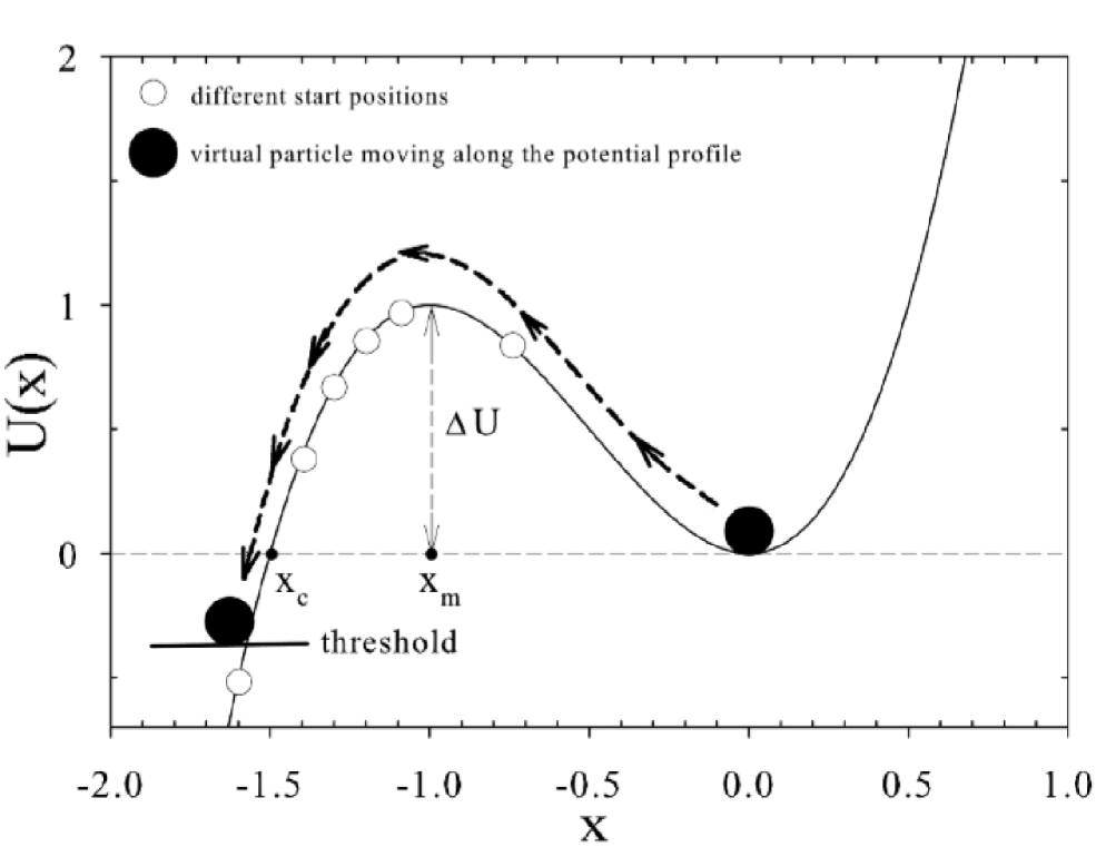
Figure 1: Cubic potential used in the dynamical equation for the process x(t) of Eq. (7). The white circles in the figure indicate the starting positions used in our simulations.

In other words, the average escape time is the mean time that a particle, starting from a certain initial point, takes to pass through a given threshold. This average time, obtained by using the backward Fokker-Planck equation, corresponds to the first passage time used in statistical physics [Redner, 2001; Inoue & Sazuka, 2007] and to the first hitting time defined in econophysics [Bonanno & Spagnolo, 2005; Montero et al., 2005].

II.1 The geometric Brownian motion model

A common starting point for many theories in economics and finance is that the stock price, in the continuous limit, is a stochastic multiplicative process defined, in the Ito sense, as

$$d\,p(t)=\gamma\cdot p(t)\cdot dt+\sigma\cdot p(t)\cdot dW(t)$$ (1)

where $\gamma$ and $\sigma$ are, in the market dynamics, the expected average growth for the price and the expected noise intensity (volatility) respectively. The price return $dp/p=d\,lnp(t)$ obeys the following additive stochastic differential equation

$$d\,lnp(t)=(\mu-\frac{\sigma^{2}}{2})\cdot dt+\sigma\cdot dW(t)\;.$$ (2)

This simple market model, proposed by Black and Scholes, catches one of the most important stylized facts of the financial markets, that is the short range correlation for price returns. This characteristic is necessary in order to warrant market efficiency.

In the geometric Brownian motion the returns are independent on each other, so the probability to observe a value after a certain barrier is given by the probability that the ”particle” doesn’t escape after $n-1$ time steps, multiplied by the escape probability at the $n^{th}$ step

$$F(\tau) = (1-p)\cdot p^{n-1}$$

$$= (1-p)\cdot exp\left[(n-1)\ln p\right],\;\;\;n=\frac{\tau}{\Delta t}$$

where $p$ is the probability to observe a return inside the region limited by the barrier, $\Delta t$ is the observation time step and $\tau$ is the escape time. So the behavior of the PF of hitting times is exponential. The geometric Brownian motion however is not adequate to describe financial market behavior. In fact the volatility is considered as a constant parameter and the PF of the price is a log-normal distribution. As a consequence many observations of real data are in clear disagreement with this model [Mantegna & Stanley, 2000; Bouchaud & Potters, 2004].

II.2 Stochastic volatility models

II.2.1 The GARCH model

Data on financial return volatility are influenced by time dependent information flow which results in pronounced temporal volatility clustering. These time series can be parameterized using Generalized Autoregressive Conditional Heteroskedastic (GARCH) models. It has been found that GARCH models can provide good in-sample parameter estimates and, when the appropriate volatility measure is used, reliable out-of-sample volatility forecasts [Anderson & Bollerslev, 1998].

The GARCH(p,q) process, which is essentially a random multiplicative process, is the generalization of the ARCH process and combines linearly the present return with the $p$ previous values of the variance and the $q$ previous values of the square return [Bollerslev, 1986]. The process is described by the equations

$$\sigma^{2}_{t} = \alpha_{0}+\alpha_{1}x^{2}_{t-1}+\dots+\alpha^{2}_{q}x^{2}_{t-q}+\beta_{1}\sigma^{2}_{t-1}$$ (4)

$$+ \dots+\beta_{p}\sigma^{2}_{t-p},\;\;\;\;\;\;\;x_{t}=\eta_{t}\cdot\sigma_{t},$$

where $\alpha_{i}$ and $\beta_{i}$ are parameters that can be estimated by means of a best fit of real market data, $\eta_{t}$ is an independent identically distributed random process with zero mean and unit variance. Using the assumption of Guassian conditional PF, $\eta_{t}$ is Gaussian. In Eq.(4) $x_{t}$ is a stochastic process representing price returns and is characterized by a standard deviation $\sigma_{t}$. The GARCH process has a non-constant conditional variance but the variance observed in long time period, called unconditional variance, is instead constant and can be calculated as a function of the model parameters. We shall consider the simpler GARCH(1,1) model

$$\sigma^{2}_{t}=\alpha_{0}+(\alpha_{1}\eta_{t-1}^{2}+\beta_{1})\sigma^{2}_{t-1},\;\;x_{t}=\eta_{t}\cdot\sigma_{t}\;.$$ (5)

The autocorrelation function of the process $x_{t}$ is proportional to a delta function, while the process $x_{t}^{2}$ has a correlation characteristic time equal to $\tau=\mid ln(\alpha_{1}+\beta_{1})\mid^{-1}$ and the unconditional variance equal to $\sigma^{2}=\alpha_{0}/(1-\alpha_{1}-\beta_{1})$. By a fitting procedure between the previous expressions of $\tau$ and $\sigma^{2}$ and the empirical values of the same quantities, we can easily estimate the three parameters $\alpha_{0}$, $\alpha_{1}$ and $\beta_{1}$ which characterize the model.

II.2.2 The Heston model

The Heston model introduced by Heston [Heston, 1993] is a commonly used stochastic volatility model. It received a great attention in the financial literature specially in connection with option pricing [Fouque et al., 2000]. The Heston model was verified empirically with both stocks [Silva & Yakovenko, 2003, Dr$\check{a}$gulescu & Yakovenko, 2002] and options [Hull & White, 1987; Hull, 2004], and good agreement with the data has been found. It was also recently investigated by econophysicists [Miccichè et al., 2002; Dr$\check{a}$gulescu & Yakovenko, 2002; Silva et al., 2004; Bonanno & Spagnolo, 2005]. The model is defined by two coupled stochastic differential equations which represent the stock dynamics by the log-normal geometric Brownian motion stock process and the Cox-Ingersoll-Ross (CIR) mean-reverting process (SDE), first introduced to model the short term interest rate [Cox et al., 1985]. By considering the log of the price $x(t)=ln~{}p(t)$ the SDEs of the model are

$$dx(t) = \left(\mu-\frac{v(t)}{2}\right)\cdot dt+\sqrt{v(t)}\cdot dW_{1}(t)$$

$$dv(t) = a(b-v(t))\cdot dt+c\sqrt{v(t)}\cdot dW_{c}(t)$$

$$dW_{c}(t) = \rho\cdot dW_{1}(t)+\sqrt{1-\rho^{2}}\cdot dW_{2}(t),\;\;$$ (6)

where $\mu$ is the trend of the market, $W_{1}(t)$ and $W_{2}(t)$ are uncorrelated Wiener processes with the usual statistical properties $<dW_{i}>\thinspace=\thinspace 0,\;$ $<dW_{i}(t)dW_{j}(t^{\prime})>\thinspace=\thinspace dt~{}\delta(t-t^{\prime})~{}\delta_{i,j}$ ($i,j=1,2$), and $\rho$ is the cross correlation coefficient between the noise sources. Here $v$ is the CIR process, which is defined by three parameters: $b$, $a$ and $c$. They represent respectively the long term variance, the rate of mean reversion to the long term variance, and the volatility of variance, often called the volatility of volatility. The stochastic volatility $v(t)$ is characterized by exponential autocorrelation and volatility clustering [Cont, 2001; Bouchaud & Potters,2004; Bonanno et al., 2006], that is alternating calm with burst periods of volatility.
We end this paragraph comparing the PF of the escape times $\tau$ of the price returns obtained from real market data with the PFs obtained by using the three previous models. We use a set of returns obtained from the daily closure prices for $1071$ stocks traded at the NYSE and continuously present in the $12-$year period $1987-1998$ (3030 trading days). From this data set we obtain the time series of the returns and we calculate the time to hit a fixed threshold starting from a fixed initial position. The parameters in the models were chosen by means of a best fit, in order to reproduce the correlation properties and the variance appropriate for real market [Bonanno et al., 2005]. We choose two thresholds to define the start and the end for the random walk. Specifically we calculate the standard deviation $\sigma_{i}$, with $i=1,\dots,1071$ for each stock over the whole 12-year period. Then we set the initial threshold at the value $-0.1\cdot\sigma_{i}$ and as final threshold the value $-2\cdot\sigma_{i}$. The thresholds are different for each stock, the final threshold is considered as an absorbing barrier. The results of our simulations together with the real market data are shown in the following Fig. 2. In this figure the exponential behavior represents the PF of the escape times for the geometric Brownian motion model, which is not adequate do describe correctly the PF of $\tau$ over the entire time axis. The GARCH model provides a better qualitative agreement with real data for lower escape times and gives the exponential behaviour in the region of large escape times. Here the geometric Brownian model reproduces well the real data, whereas the Heston model is able to reproduce almost entirely the empirical PF.

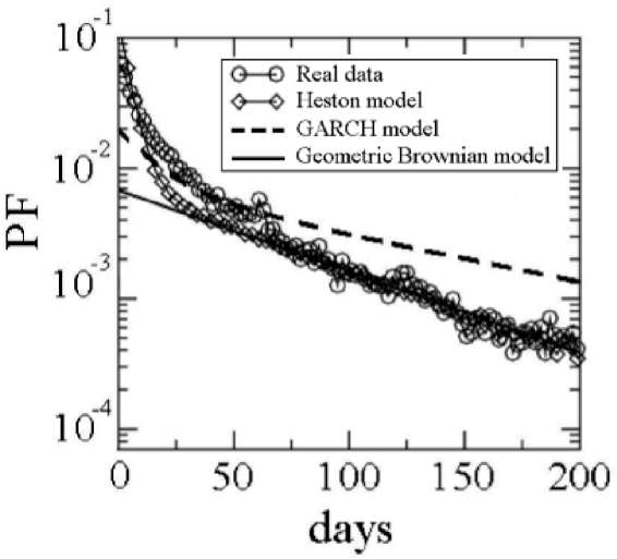
Figure 2: Probability function (PF) of escape times of stock price returns for: real market data (circle), geometric Brownian motion model (black solid line), GARCH model (black broken line) and Heston model (diamond).

II.3 The nonlinear Heston model (NLH)

To consider feedback effects on the price fluctuations and different dynamical regimes, similarly to what happens in financial markets during normal activity and in special days with relatively strong variations of the price [Bouchaud & Potters, 2004; Bouchaud & Cont, 1998; Bouchaud, 2001; Bouchaud, 2002; Bonanno et al., 2006; Bonanno et al., 2007], we proposed a generalization of the Heston model, by considering a cubic nonlinearity in the SDE of the $log$ of the price $x(t)=ln~{}p(t)$ (first equation in (6)) [Bonanno et al., 2006; Bonanno et al., 2007]. This nonlinearity allows us to describe these different dynamical regimes by the motion of a fictitious ”Brownian particle” moving in an effective potential with a metastable state. The equations of the new model are obtained by replacing in Eqs. (6) the parameter $\mu$ with the negative derivative of the nonlinear cubic potential

$$dx(t) = -\left(\frac{\partial U}{\partial x}+\frac{v(t)}{2}\right)dt+\sqrt{v(t)}dW_{1}(t)\;\;\;\;\;$$ (7)

$$dv(t) = a(b-v(t))dt+c\sqrt{v(t)}dW_{c}(t)$$ (8)

$$dW_{c}(t) = \rho dW_{1}(t)+\sqrt{1-\rho^{2}}dW_{2}(t),$$ (9)

where $U(x)=2x^{3}+3x^{2}$ is the effective cubic potential with a metastable state at $x_{me}=0$, a maximum at $x_{m}=-1$, and a cross point between the potential and the $x$ axes at $x_{c}=-1.5$ (see Fig. 1). The average exit time of the system from the stable to the unstable domain of the potential shown in Fig. 1 may be prolonged by imposing external noise: this phenomenon is named noise enhanced stability (NES). The stability of systems with a metastable state can be increased by enhancing the lifetime of the metastable state or the average exit time of the system from the well. The NES effect was experimentally observed in a tunnel diode [Mantegna & Spagnolo, 1996] and in an underdamped Josephson junction [Sun et el., 2007] and theoretically predicted in a wide variety of systems such as chaotic map, Josephson junctions, neuronal dynamics models and tumor-immune system models [Mielke, 2000; Agudov & Spagnolo, 2001; Dubkov et al., 2004; Pankratova et al., 2004; Pankratov & Spagnolo, 2004; Fiasconaro et al., 2005; Fiasconaro et al., 2006]. Two different dynamical regimes are observed depending on the initial position of the Brownian particle along the potential profile. One is characterized by a nonmonotonic behavior of the lifetime, as a function of the noise intensity (here the volatility $v(t)$), for initial positions $x_{o}<x_{c}$. The other one features a divergence of the lifetime when the noise tends to zero for initial positions $x_{c}<x_{o}<x_{m}$, implying that the Brownian particle remains trapped inside the metastable state in the limit of small noise intensities. In this dynamical regime a nonmonotonic behavior of the lifetime with a minimum and a maximum as a function of the noise intensity is also observed. This trapping phenomenon is always observable when initial unstable positions of the Brownian particle are near a metatastable state of the system investigated. The NES effect and its different dynamical regimes can be explained considering the barrier ”seen” by the Brownian particle starting at the initial position $x_{o}$, that is $\Delta U_{in}=U(x_{max})-U(x_{o})$, and by comparing it with the height of the barrier $\Delta U$ characterizing the metastable state (see Fig. 1) [Agudov & Spagnolo, 2001; Fiasconaro et al., 2005]. For example for unstable initial positions such as $x_{c}<x_{o}<x_{m}$ we have $\Delta U_{in}<\Delta U$ and from a probabilistic point of view, it is easier to enter into the well than to escape from, once the particle is entered. So a small amount of noise can increase the lifetime of the metastable state. When the noise intensity $v$ is much greater than $\Delta U$, the typical exponential behavior is recovered.
By investigating the mean escape time (MET), as a function of the model parameters $a$, $b$ and $c$, we found the parameter region where a nonmonotonic behavior of MET is observable in our NLH model with stochastic volatility $v(t)$ [Bonanno et al., 2006; Bonanno et al., 2007]. This behaviour is similar to that observed for MET versus $v$ in the NES effect with constant volatility $v$. We call the enhancement of the mean escape time (MET), with a nonmonotonic behavior as a function of the model parameters, NES effect in a broad sense. Two limit regimes characterize our NLH model, one corresponding to the case $a=0$, with only the noise term in the equation for the volatility $v(t)$, and the other one corresponding to the case $c=0$ with only the reverting term in the same Eq. (8). In the first case ($a=0$), the system becomes too noisy and the NES effect is not observable in the behavior of MET as a function of the parameter $c$. In the second case ($c=0$), after an exponential transient, the volatility reaches the asymptotic value $b$, and the NES effect is observable as a function of $b$. This case corresponds to the usual constant volatility regime.
By considering the two noise sources $W_{1}(t)$ and $W_{c}(t)$ of Eqs. (7) and (8) completely uncorrelated ($\rho=0$), the results of simulations of the NLH model (Eqs. (7)-(9)), in the second case ($c=0$), are reported in Fig. 3, where MET versus $b$ is plotted for three different starting unstable initial positions and for $c=0$.

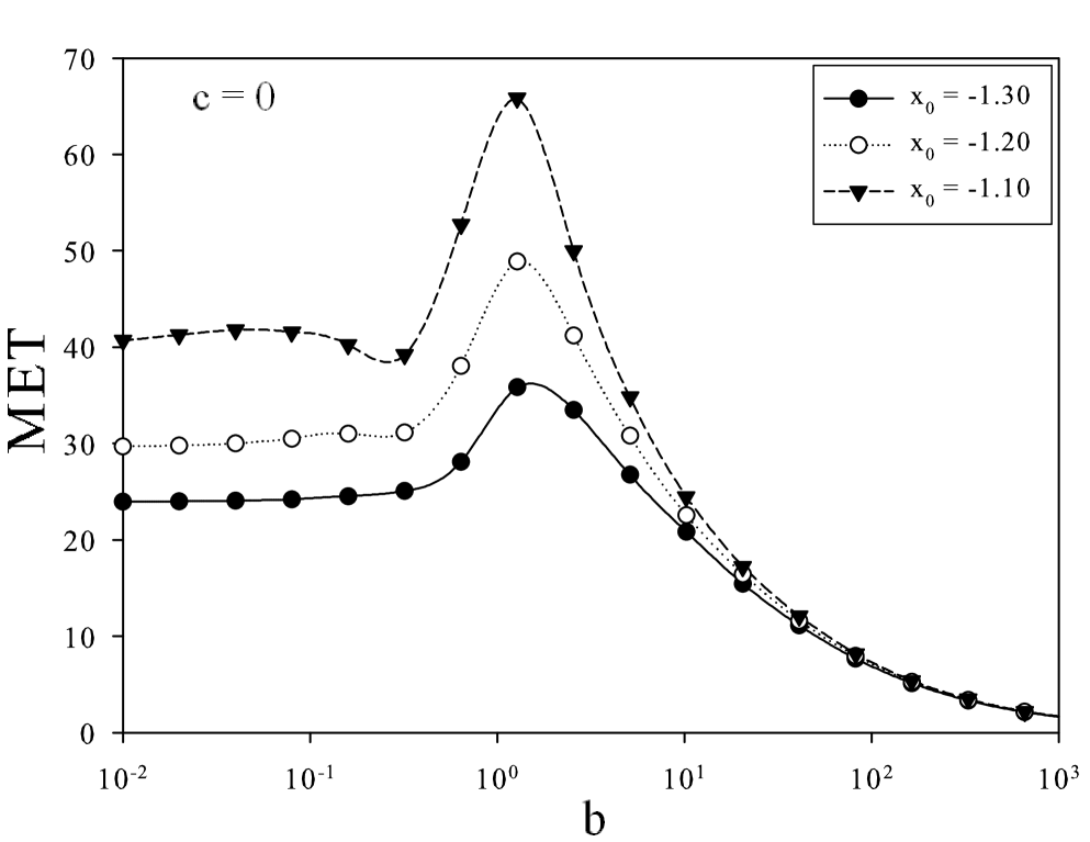
Figure 3: Mean escape time (MET) for $3$ different unstable starting positions, when only the reverting term is present: $a=10^{-2}$, $c=0$. The curves are averaged over $10^{5}$ escape events.

The simulations were performed considering the initial positions of the process $x(t)$ in the unstable region $[x_{c},x_{m}]$ and using an absorbing barrier at $x=-6.0$. When the process $x(t)$ hits the barrier, the escape time is registered and another simulation is started, placing the process at the same starting position $x_{o}$, but using the volatility value of the barrier hitting time. The nonmonotonic behavior, which is more evident for starting positions near the maximum of the potential, is always present. After the maximum, when the values of $b$ are much greater than the potential barrier height, the exponential behavior is recovered. The results of our simulations show that the NES effect can be observed as a function of the volatility reverting level $b$, the effect being modulated by the parameter $(ab)/c$. The phenomenon disappears if the noise term is predominant in comparison with the reverting term. Moreover the effect is no more observable if the parameter $c$ pushes the system towards a too noisy region. When the noise term is coupled to the reverting term, we observe the NES effect as a function of the parameter $c$. The effect disappears if $b$ is so high as to saturate the system.
In financial markets the log of the price $x(t)=ln~{}p(t)$ and the volatility $v(t)$ can be correlated ($\rho\neq 0$), and a negative correlation between the processes is known as leverage effect [Fouque et al., 2000]. A negative correlation between the logarithm of the price and the volatility means that a decrease in $x(t)$ induces an increase in the volatility $v(t)$, and this causes the Brownian particle to escape easily from the well. As a consequence the mean lifetime of the metastable state decreases, even if the nonmonotonic behavior is still observable. On the contrary, when the correlation $\rho$ is positive, decrease in $x(t)$ indeed is associated with decrease in the volatility, the Brownian particle therefore stays more inside the well. The escape process becomes slow and this increases further the lifetime of the metastable state. The presence of correlation between the stochastic volatility and the noise source which affects directly the dynamics of the quantity $x(t)=\ln p(t)$ (as in usual market models) can influence therefore the stability of the market. Specifically a positive correlation between $x(t)$ and volatility $v(t)$ slows down the walker escape process, that is it delays the crash phenomenon increasing the stability of the market. Conversely a negative correlation accelerates the escape process, lowering the stability of the system [Bonanno et al., 2006].

III Role of the initial conditions and statistical features

In this last section we study, for the uncorrelated ($\rho=0$) NHL model (Eqs. (7)-(9)), the role of the initial position of the fictitious Brownian particle on the mean escape time (MET). In particular we fix an escape barrier (threshold) and we analyze the behaviour of MET as a function of $a$, $b$ and $c$ (CIR process parameters) for different start positions (see Fig 1). First we consider the behavior of MET as a function of the reverting term $b$. In Fig. 4 (panel (a) of part (A)) we show the curves averaged on $10^{7}$ escape events. The curves inside all the other panels have been obtained averaging on $10^{5}$ realizations. In our simulations we consider two different values of the parameter $c$, namely $c=10^{-2},10$, and eight values of the parameter $a$, that is: (A) $a=10^{-7},10^{-6},10^{-4},10^{-1}$; and (B) $a=10^{-1},1,10,10^{2}$. Each panel corresponds to a different value of initial position, namely: (a) $x_{o}=-0.75$, (b) $x_{o}=-1.10$, (c) $x_{o}=-1.40$, (d) $x_{o}=-1.60$. Inside each panel different curves correspond to different values of $a$. First of all we comment the panels (b), (c) and (d) of part (A), related to unstable initial positions outside the potential well. The nonmonotonic shape, characteristic of the NES effect, is clearly shown in these three panels. This behavior is shifted towards higher values of $b$ as the parameter $a$ decreases, and it is always present. The NES effect is more pronounced for initial positions near the top of the potential barrier.

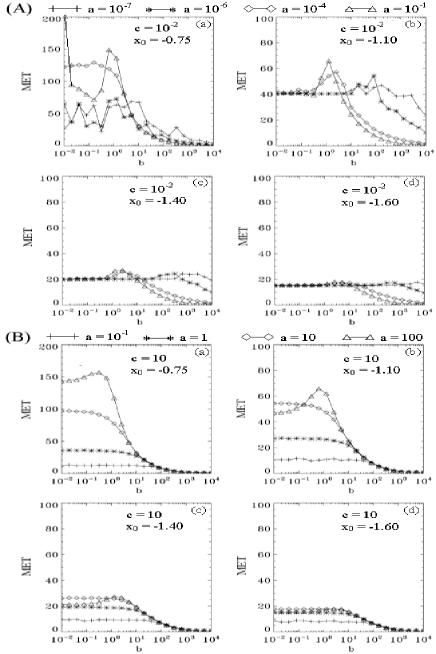
Figure 4: Mean escape time (MET) as a function of reverting level $b$. (A) $c=10^{-2}$, (B) $c=10$. Each panel corresponds to different values of initial position. Inside each panel different curves correspond to different values of $a$.

For initial positions far from the maximum of the potential, the trapping event becomes less probable. To obtain a more pronounced NES effect we should consider very low values of the absorbing barrier, that is $x\ll-6$, which are meaningless from financial market point of view. For the higher value $c=10$, we observe the nonmonotonic behavior only for a very great value of the parameter $a$, that is for $a=100\gg c$ (see panels (b), (c), (d) of Fig. 4B). For further increase of the parameter $c$ the noise experienced by the system is much greater than the effective potential barrier ”seen” by the fictitious Brownian particle and the NES effect is never observable. We note that the parameters $a$ and $c$ play a regulatory role in Eq. (8). In fact for $a\gg c$ the drift term is predominant while for $a\ll c$ the dynamics is driven by the noise term, unless the parameter $b$ takes great values. The nonmonotonic behavior is observed for $a\ll c$, provided that $b\gg c$. For increasing values of $a$ the system approaches the revert-only regime and we recover the behavior shown in Fig. 3.
Now we consider the panel of Fig 4A related to the unstable initial position outside the potential well. For very low values of the parameter $a$ the nonmonotonic behavior is absent and the mean escape time (MET) decreases monotonically with strong fluctuations. We recover the similar behavior obtained in the limit case of $a=0$ and discussed in [Bonanno et al., 2007]. For $a\ll c$, in fact, we can neglect the reverting term in Eq. (8) and the volatility is proportional to the square of the Wiener process. The dynamics is dominated by the noise term with large fluctuations for the MET. This behavior is mainly due to the presence of the Ito term in Eq. (7) for log returns $x(t)$. The Ito term modifies randomly the potential shape of Fig. 1 in such a way that the potential barrier disappears for greater values of the volatility $v(t)$, producing a random enhancement of the escape process. Increasing the value of $a$ these fluctuations disappear because the reverting term becomes more important. This is the behavior shown for $a=10^{-4}$. A further increase of $a$ causes the revert term to dominate the dynamics with respect to the noise term. Moreover, because the initial unstable position $x_{o}=-0.75$ is near the maximum of the potential well, we recover the divergent dynamical regime characterized by a nonmonotonic behavior with a minimum and a maximum of MET as a function of the noise intensity, here represented by the parameter b [Fiasconaro et al., 2005]. For very low values of $b$, the fictitious Brownian particle is trapped inside the potential well with a divergence of MET in the limit $b\rightarrow 0$. For increasing $b$ the particle can escape more easily, and the MET decreases, as long as the noise intensity, represented by the parameter $b$, reaches the value $0.15$ corresponding to the barrier height $\Delta U_{in}$ ”seen” by the particle. Close to this value of $b$, the escape process is slowed down, because the probability of reentering the well is equal to that of escaping from. This behavior is represented by the minimum of MET at $b\simeq 0.15$ in the panel (a) of Fig. 4A. By increasing $b$, the particle escaped from the well can reenter as long as the noise intensity is comparable with the height of the potential barrier. The MET therefore increases until reach a maximum at $b\simeq\Delta U=1$. At higher values of $b$, one recovers a monotonic decreasing behavior of the MET. The same nonmonotonic behavior with a minimum and a maximum is visible in Fig. 3 for $x_{o}=-1.10$.

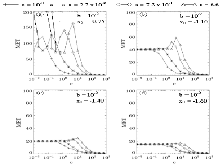
Figure 5: Mean escape time (MET) as a function of the noise intensity $c$ for a fixed value of $b$ ($b=10^{-2}$). Each panel corresponds to different values of initial condition as in Fig 4. Inside each panel different curves correspond to the following values of $a$: cross $10^{-3}$, star $2.7\times 10^{-2}$, diamond $7.3\times 10^{-1}$, triangle $6.6$.

Now we consider the dependence of MET on the noise intensity $c$. Fig. 5 shows the curves of MET versus $c$, averaged over $10^{5}$ escape events in panels (b), (c), (d) and $10^{6}$ escape events in panel (a). First of all we consider the unstable initial positions outside the well, that is panels (b), (c) and (d). Each panel corresponds to a different value of initial position as in Fig 4. Inside each panel different curves correspond to different values of $a$. The shape of the curves is similar to that observed in Fig. 4. Specifically for small values of $a$, when the reverting term is negligible, the absence of the nonmonotonic behavior is expected. By increasing $a$ the nonmonotonic behavior is recovered. Again the NES effect is more pronounced for initial positions near the maximum of the potential. For initial position inside the potential well as in panel (a), we observe a divergent behavior of MET for three values of the parameter $a$ (namely $a=2.7\cdot 10^{-2},7.3\cdot 10^{-1},6.6$), because of the small value of $b=10^{-2}$. Recall that the volatility $v(t)$ reverts towards a long term mean squared volatility $b$ with relaxation time given by $a^{-1}$. So, for increasing values of $a$ the Brownian fictitious particle experiences the low value of the noise intensity $b=10^{-2}$ in a shorter time and therefore the particle is trapped for relatively small values of $c$ (see the curves for $a=7.3\cdot 10^{-1}$ and $a=6.6$). By decreasing the value of $a$, the relaxation time increases considerably and the trapping of the particle occurs for lower values of $c$ (see the curve for $a=2.7\cdot 10^{-2}$). For the lowest value, $a=10^{-3}$, we recover the regime of strong fluctuations due to the predominance of the noise term with respect to the revert term in Eq. (8). The fluctuating behavior of all the curves before the divergence in Fig. 5 is also due to this effect.
It is interesting to show, for our NLH model (Eqs. (7)-(9)), some of the well-established statistical features of the financial time series, such as the probability function (PF) of the stock price returns, the PF of the volatility and the return correlation, and to compare them with the same characteristics obtained from real market data. As initial position we choose $x_{o}=-0.75$. For this start point, located inside the well, we have very interesting behavior of the MET as a function of the noise intensity $b$ (see panel (a) of Fig 4A). In Fig. 6 we show the PF of the returns. To characterize quantitatively this PF with regard to the width, the asymmetry and the fatness of the distribution, we calculate the mean value $<\Delta x>$, the variance $\sigma_{\Delta x}$, the skewness $\kappa_{3}$, and the kurtosis $\kappa_{4}$ for the NLH model and for real market data. We obtain for real data: $<\Delta x>=0.221\cdot 10^{-3}$, $\sigma_{\Delta x}=0.0221$, $\kappa_{3}=-1.353$, $\kappa_{4}=79.334$; for the NLH model: $<\Delta x>=-1.909\cdot 10^{-5}$, $\sigma_{\Delta x}=0.0246$, $\kappa_{3}=-4.3501$, $\kappa_{4}=441.65$. The agreement between theoretical results and real data is quite good except at high values of the returns. These statistical quantities clearly show the asymmetry of the distribution and its leptokurtic nature observed in real market data. In fact, the empirical PF is characterized by a narrow and large maximum, and fat tails in comparison with the Gaussian distribution [Mantegna & Stanley, 2000; Bouchaud & Potters, 2004].

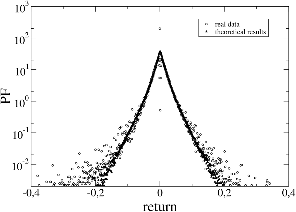
Figure 6: Probability function of the stock price returns: (a) real data (circle), (b) NLH model (Eqs. (7)-(9)) (triangle). The values of the parameters are: $a=2.00$, $b=0.01$, $c=0.75$, $x_{0}=-0.75$, $x_{abs}=-6.0$, $v_{start}=8.62\times 10^{-5}$.

In Fig. 7 we show the PF of the volatility for our model, and we can see a log-normal behavior as that observed approximately in real market data. The agreement is very good for values of the volatility greater than $v\sim 0.03$ and discrepancies are in the range of very low volatility values.

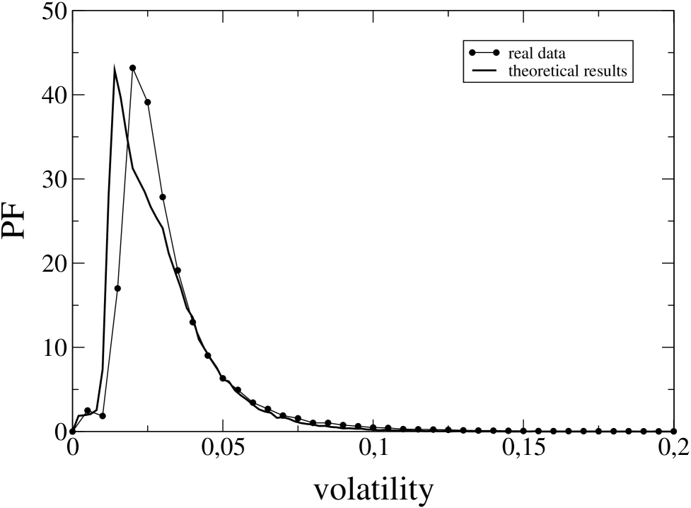
Figure 7: Probability function of the volatility: (a) real data (black circle), (b) NLH model (Eqs. (7)-(9)) (solid line). The values of the parameters are the same as in Fig. 6.

Finally in Fig. 8a we show the correlation function of the returns for NLH model and for the real data. The agreement of the two correlation functions is very good for all the time. As we can see, the autocorrelations of the asset returns are insignificant, except for very small time scale for which microstructure effects come into play. This is in agreement with one of the stylized empirical facts emerging from the statistical analysis of price variations in various types of financial markets [Cont, 2001]. The good agreement between theoretical and experimental behaviour is confirmed by the correlation function of the logarithmic absolute returns, which decays slowly to zero (see Fig. 8b).

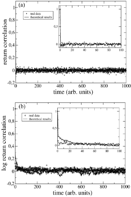
Figure 8: (a) Correlation function of returns (panel a) and log absolute returns (panel b): real data (circle), NLH model (Eqs. (7) - (9)) (solid line). Inset: detail of the behaviour at short times. The values of the parameters are the same of Fig. 6. Inset: detail of the behaviour at short times.

Our last investigation concerns the PF of the escape time of the returns, which is the main focus of our paper.

Figure 9: Probability function of the escape time of the returns from simulation (solid line), and from real data (black circle). The values of the thresholds are: $\Delta x_{i}=-0.1\thinspace\sigma_{\Delta x}$, $\Delta x_{f}=-1.5\thinspace\sigma_{\Delta x}$. The values of the other parameters are the same as in Fig. 6

By using our model (Eqs. (7)-(9)), we calculate the probability function for the escape time of the returns. We define two thresholds, $\Delta x_{i}$ and $\Delta x_{f}$, which represent the start point and the end point respectively for calculating MET. To fix the values of the two thresholds we consider the standard deviation (SD) $\sigma_{\Delta x}$ of the return series over a long time period corresponding to that of the real data and we set $\Delta x_{i}=-0.1\thinspace\sigma_{\Delta x}$, $\Delta x_{f}=-1.5\thinspace\sigma_{\Delta x}$. The initial position is $x_{0}=-0.75$ and the absorbing barrier is at $x_{abs}=-6.0$. We use a trial and error procedure to select the values of the parameters $a$, $b$, and $c$ for which we obtain the best fitting between all the statistical features considered, theoretical (NLH model) and empirical (real data). As real data we use the daily closure prices for $1071$ stocks traded at the NYSE and continuously present in the $12-$year period $1987-1998$ (3030 trading days). In Fig. 9 we report the results for the PF of the escape times obtained both from real and theoretical data: we note a good qualitative agreement between the two PFs. Moreover we check the agreement between the two data sets by performing both $\chi^{2}$ and Kolmogorov-Smirnov (K-S) goodness-of-fit tests. The results are: $\chi^{2}\thinspace=\thinspace 0.01620$, $\tilde{\chi}^{2}\thinspace=\thinspace 0.00017$ ($\tilde{\chi}^{2}$ indicates the reduced $\chi^{2}$) and $D=0.14$, $P=0.261$, where $D$ and $P$ are respectively the maximum difference between the cumulative distributions and the corresponding probability for the K-S test. The results obtained from both tests indicate that the two distributions of Fig. 9 are not significantly different. Of course, a better quantitative fitting procedure could be done by considering also the potential parameters. This detailed analysis will be done in a forthcoming paper.

IV Conclusions

We studied the statistical properties of the escape times in different models for stock market evolution. We compared the PFs of the escape times of the returns obtained by the basic geometric Brownian motion model and by two commonly used SV models (GARCH and Heston models) with the PF of real market data. Our results indeed show that to fit well the escape time distribution obtained from market data, it is necessary to take into account the stochasticity of the volatility. In the nonlinear Heston model, recently introduced by the authors, after reviewing the role of the CIR parameters on the dynamics of the model, we analyze in detail the role of the initial conditions on the escape time from a metastable state. We found that the NES effect, which could be considered as a measure of the stabilizing effect of the noise on the marked dynamics, is more pronounced for unstable initial positions near the maximum of the potential. For initial positions inside the potential well we recover an interesting nonmonotonic behavior with a minimum and a maximum for the MET as a function of the parameter $b$. This behaviour is a typical signature of the NES effect in the divergent dynamical regime [Fiasconaro et al., 2005]. To check the reliability of our NLH model we compare the return correlation function, the PFs of the returns, the volatility and the escape times with the corresponding ones obtained from real market data. We find good agreement for some of these characteristics.

References

- Agudov, N. V. & Spagnolo, B., (2001) Agudov, N. V. & Spagnolo, B., [2001] ”Noise enhanced stability of periodically driven metastable states,” Phys. Rev. E 64 035102(R)(4).
- Anderson, P. W., Arrow, K. J. & Pines, D., (1988) Anderson, P. W., Arrow, K. J. & Pines, D. [1988] The Economy as An Evolving Complex System I (Addison Wesley Longman, Redwood City, California).
- Anderson, P. W., Arrow, K. J. & Pines, D., (1997) Anderson, P. W., Arrow, K. J. & Pines, D. [1997] The Economy as An Evolving Complex System II (Addison Wesley Longman, Redwood City, California).
- Anderson, T. & Bollerslev, T., (1998) Anderson, T. & Bollerslev, T. [1998] ”Answering the Skeptics: Yes, Standard Volatility models do provide accurate forecasts,” International Economic Review 39, No 4, 885-905.
- Black, F. & Scholes, M., (1973) Black, F. & Scholes, M. [1973] ”Valuation of options and corporate liabilities,” J. Political Economy 81, 637-654.
- Bollerslev, T., (1986) Bollerslev, T. [1986] ”Generalized autoregressive conditional heteroskedasticity,” J. Econometrics 31, 307-327.
- Bonanno, G. & Spagnolo, B., (2005) Bonanno, G. & Spagnolo, B. [2005] ”Escape times in stock markets,” Fluctuation and noise letters 5 (2), L325-L330.
- Bonanno, G., Valenti, D., Spagnolo, B., (2006) Bonanno, G., Valenti, D., Spagnolo, B. [2006] ”Role of noise in a market model with stochastic volatility,” Eur. Phys. J. B 53, 405-409.
- Bonanno, G., Valenti, D., Spagnolo, B., (2007) Bonanno, G., Valenti, D., Spagnolo, B. [2007] ”Mean escape time in a system with stochastic volatility,” Phys. Rev. E 75, 016106 (8).
- Borland, L., (2002) Borland, L. [2002] ”A theory of non-Gaussian option pricing,” Quantitative Finance 2, 415-431 (2002).
- (11) Borland, L. [2002b] ”Option Pricing Formulas Based on a Non-Gaussian Stock Price Model,” Phys. Rev. Lett. 89, 098701 (4).
- Bouchaud, J.-P., (2001) Bouchaud, J.-P. [2001] ”Power laws in economics and finance: some ideas from physics,” Quantitative Finance 1, 105-112.
- Bouchaud, J.-P., (2002) Bouchaud, J.-P. [2002] ”An introduction to statistical finance,” Physica A 313, 238-112.
- Bouchaud, J.-P. & Cont, R., (1998) Bouchaud, J.-P. & Cont, R. [1998] ”A Langevin approach to stock market fluctuations and crashes,” Eur. Phys. J. B 6, 543-550.
- Bouchaud, J. P. & Potters, M., (2004) Bouchaud, J. P. & Potters, M. [2004] Theory of Financial Risks and Derivative Pricing (Cambridge University Press, Cambridge).
- Cont, R., (2001) Cont, R. [2001] ”Empirical properties of asset returns: stylized facts and statistical issues,” Quantitative Finance 1, 223-236.
- Cox, J. Ingersoll, J. & Ross, S., (1985) Cox, J. Ingersoll, J. & Ross, S. [1985] ”A theory of the term structure of interest rates”, Econometrica 503, 385-407.
- Dacorogna, M. M., Gencay, R., Müller, U. A., Olsen, R. B. & Pictet, O.V., (2001) Dacorogna, M. M., Gencay, R., Müller, U. A., Olsen, R. B. & Pictet, O.V. [2001] An Introduction to High-Frequency Finance (Academic Press, New York).
- Drgulescu, A. A. & Yakovenko, V. M., (2002) Drgulescu, A. A. & Yakovenko, V. M. [2002] ”Probability distribution of return in the Heston model with stochastic volatility,” Quantitative Finance 2, 443-453.
- Dubkov, A. A., Agudov, N. V. & Spagnolo, B., (2004) Dubkov, A. A., Agudov, N. V. & Spagnolo, B. [2004] ”Noise enhanced stability in fluctuating metastable states,” Phys. Rev. E 649 061103(7).
- Engle, R. F., (1982) Engle, R. F. [1982] ”Autoregressive conditional heteroskedasticity with estimates of the variance of U.K. inflation,” Econometrica 50, 987-1002.
- Fiasconaro, A., Spagnolo, B. & Boccaletti, S., (2005) Fiasconaro, A., Spagnolo, B. & Boccaletti, S. [2005] ”Signatures of noise-enhanced stability in metastable states,” Phys. Rev. E 72, 061110(5).
- Fiasconaro, A., Spagnolo, B., Ochab-Marcinek, A. & Gudowska-Nowak, E., (2006) Fiasconaro, A., Spagnolo, B., Ochab-Marcinek, A. & Gudowska-Nowak, E. [2006] ”Co-occurrence of resonant activation and noise-enhanced stability in a model of cancer growth in the presence of immune response,” Phys. Rev. E 74, 041904(10).
- Fouque, J. P., Papanicolaou, G. & Sircar K. R., (2000) Fouque, J. P., Papanicolaou, G. & Sircar K. R. [2000] Derivatives in financial markets with stochastic volatility (Cambridge University Press, Cambridge). The volatility smile is the shape of the curve of the implied volatility, for option prices in Black-Scholes model, as a function of the strike price.
- Gardiner, C. W., (2004) Gardiner, C. W. [2004] Handbook of Stochastic Methods4 (Springer-Verlag, Berlin).
- Adhya, S. and Merril, C., (2006) Hatchett, J. P. L. & Khn, R. [2006] ”Effects of economic interactions on credit risk,” J. Phys. A 39, 2231-2251.
- Heston, S. L., (1993) Heston, S. L. [1993] ”A closed-form solution for options with stochastic volatility with applications to bond and currency options,” Rev. Financial Studies 6, 327-343.
- Hull, J., (2004) Hull, J. [2004] Options, Futures, and Other Derivatives (Prentice-Hall, New York).
- Hull, J. & White, A., (1987) Hull, J. & White, A. [1987] ”The Pricing of Options on Assets with Stochastic Volatilities,” J. Finance XLII, 281-300.
- Inoue, J., Sazuka, N., (2007) Inoue, J., Sazuka, N. [2007] ”Crossover between Lévy and Gaussian regimes in first-passage processes,” Phys. Rev. E 76, 021111.
- Malcai, O., Biham, O., Richmond, P. & S. Solomon, (2002) Malcai, O., Biham, O., Richmond, P. & S. Solomon [2002] ”Theoretical analysis and simulations of the generalized Lotka-Volterra model,” Phys. Rev. E 66, 031102(6).
- Mantegna, R. N. & Spagnolo, B., (1996) Mantegna, R. N. & Spagnolo, B. [1996] ”Noise Enhanced Stability in an Unstable System,” Phys. Rev. Lett. 76, 563-566.
- Adhya, S. and Merril, C., (2006) Mantegna, R. N. & Stanley, H. E. [2000] An Introduction to Econophysics: Correlations and Complexity in Finance (Cambridge University Press, Cambridge).
- Miccichè, S., Bonanno, G., Lillo, F. & Mantegna, R. N., (2002) Miccichè, S., Bonanno, G., Lillo, F. & Mantegna, R. N. [2002] ”Volatility in financial markets: stochastic models and empirical results,” Physica A 314, 756-761.
- Mielke, A., (2000) Mielke, A. [2000] ”Noise Induced Stability in Fluctuating, Bistable Potentials,” Phys. Rev. Lett. 84, 818-821.
- Montero, M., Perell, J., Masoliver, J., Lillo, F., Miccich, S. & Mantegna, R. N., (2005) Montero, M., Perell, J., Masoliver, J., Lillo, F., Miccich, S. & Mantegna, R. N. [2005] ”Scaling and data collapse for the mean exit time of asset prices,” Phys. Rev. E 72, 056101(10).
- Pankratov, A. L. & Spagnolo, B, (2004) Pankratov, A. L. & Spagnolo, B [2004] ”Suppression of time errors in short overdamped Josephson junctions,” Phys. Rev. Lett. 93, 177001(4).
- Pankratova, E. V., Polovinkin, A. V. & Spagnolo, B., (2004) Pankratova, E. V., Polovinkin, A. V. & Spagnolo, B. [2004] ”Suppression of noise in FitzHugh-Nagumo model driven by a strong periodic signal,” Phys. Lett. A, 344 43-50.
- Raberto, M., Scalas, E. & F. Mainardi, F., (2002) Raberto, M., Scalas, E. & F. Mainardi, F. [2002] ”Waiting-times and returns in high-frequency financial data: an empirical study,” Physica A 314, 749-755.
- Redner, S., (2001) Redner, S. [2001] A Guide to First-Passage Processes (Cambridge University Press, Cambridge, England).
- Silva, A. C., Prange, R. E. & Yakovenko, V. M., (2004) Silva, A. C., Prange, R. E. & Yakovenko, V. M. [2004] ”Exponential distribution of financial returns at mesoscopic time lags: a new stylized fact,” Physica A 344, 227-235.
- Silva, A. C. & Yakovenko, V. M., (2003) Silva, A. C. & Yakovenko, V. M. [2003] ”Comparison between the probability distribution of returns in the Heston model and empirical data for stock indexes,” Physica A 324, 303-310.
- Sornette, D., (2003) Sornette, D. [2003] ”Critical market crashes,” Physics Reports 378, 1 98.
- Sun, G. et al., (2007) Sun, G. et al. [2007] ”Thermal escape from a metastable state in periodically driven Josephson junctions,” Phys. Rev. E 75, 021107(4).