Distributed Kalman Filter
via Gaussian Belief Propagation

Abstract

Recent result shows how to compute distributively and efficiently the linear MMSE for the multiuser detection problem, using the Gaussian BP algorithm. In the current work, we extend this construction, and show that operating this algorithm twice on the matching inputs, has several interesting interpretations. First, we show equivalence to computing one iteration of the Kalman filter. Second, we show that the Kalman filter is a special case of the Gaussian information bottleneck algorithm, when the weight parameter $\beta=1$. Third, we discuss the relation to the Affine-scaling interior-point method and show it is a special case of Kalman filter.

Besides of the theoretical interest of this linking estimation, compression/clustering and optimization, we allow a single distributed implementation of those algorithms, which is a highly practical and important task in sensor and mobile ad-hoc networks. Application to numerous problem domains includes collaborative signal processing and distributed allocation of resources in a communication network.

I Introduction

Recent work [1] shows how to compute efficiently and distributively the MMSE prediction for the multiuser detection problem, using the Gaussian Belief Propagation (GaBP) algorithm. The basic idea is to shift the problem from linear algebra domain into a probabilistic graphical model, solving an equivalent inference problem using the efficient belief propagation inference engine. [2] compares the empirical performance of the GaBP algorithm relative to other linear iterative algorithms, demonstrating faster convergence. [3] elaborates on the relation to solving systems of linear equations.

In the present work, we propose to extend the previous construction, and show, that by performing the MMSE computation twice on the matching inputs we are able to compute several algorithms. First, we reduce the discrete Kalman filter computation [4] to a matrix inversion problem and show how to solve it using the GaBP algorithm. We show that Kalman filter iteration which is composed from prediction and measurement steps can be computed by two consecutive MMSE predictions. Second, we explore the relation to Gaussian information bottleneck (GIB) [5] and show that Kalman filter is a special instance of the GIB algorithm, when the weight parameter $\beta=1$. To the best of the authors knowledge, this is the first algorithmic link between the information bottleneck framework and linear dynamical systems. Third, we discuss the connection to the Affine-scaling interior-point method and show it is an instance of the Kalman filter.

Besides of the theoretical interest of linking compression, estimation and optimization together, our work is highly practical since it proposes a general framework for computing all of the above tasks distributively in a computer network. This result can have many applications in the fields of estimation, collaborative signal processing, distributed resource allocation etc.

A closely related work is [6]. In this work, Frey et al. focus on the belief propagation algorithm (a.k.a sum-product algorithm) using factor graph topologies. They show that the Kalman filter algorithm can be computed using belief propagation over a factor graph. In this contribution we extend their work in several directions. First, we extend the computation to vector variables (relative to scalar variables in Frey’s work). Second, we use a different graphical model: an undirected graphical model which results in simpler update rules, where Frey uses factor-graph with two types of messages: factor to variables and variables to factors. Third and most important, we allow an efficient distributed calculation of the Kalman filter steps, where Frey’s algorithm is centralized.

Another related work is [7]. In this work the link between Kalman filter and linear programming is established. In this work we propose a new and different construction which ties the two algorithms.

The structure of this paper is as follows. In Section II we describe the discrete Kalman filter. In Section III we outline the GIB algorithm and discuss its relation to the Kalman filter. Section IV presents the Affine-scaling interior-point method and compares it to the Kalman filter algorithm. Section V presents our novel construction for performing an efficient distributed computation of the three methods.

II Kalman Filter

II-A An Overview

The Kalman filter is an efficient iterative algorithm to estimate the state of a discrete-time controlled process $x\in R^{n}$ that is governed by the linear stochastic difference equation :

$$x_{k}=Ax_{k-1}+Bu_{k-1}+w_{k-1},$$ (1)

with a measurement $z\in R^{m}$ that is $z_{k}=Hx_{k}+v_{k}.$ The random variables $w_{k}$ and $v_{k}$ that represent the process and measurement AWGN noise (respectively). $p(w)\sim\mathcal{N}(0,Q),p(v)\sim\mathcal{N}(0,R)$. We further assume that the matrices $A,H,B,Q,R$ are given.

The discrete Kalman filter update equations are given by [4]:

The prediction step:

$$\hat{x}^{-}_{k} = A\hat{x}_{k-1}+Bu_{k-1},$$ (2a)

$$P_{k}^{-} = AP_{k-1}A^{T}+Q.$$ (2b)

The measurement step:

$$K_{k} = P_{k}^{-}H^{T}(HP_{k}^{-}H^{T}+R)^{-1},$$ (3a)

$$\hat{x}_{k} = \hat{x}^{-}_{k}+K_{k}(z_{k}-H\hat{x}^{-}_{k}),$$ (3b)

$$P_{k} = (I-K_{k}H)P_{k}^{-}.$$ (3c)

where $I$ is the identity matrix.

The algorithm operates in rounds. In round $k$ the estimates $K_{k},\hat{x}_{k},P_{k}$ are computed, incorporating the (noisy) measurement $z_{k}$ obtained in this round. The output of the algorithm are the mean vector $\hat{x}_{k}$ and the covariance matrix $P_{k}$.

II-B New construction

Our novel contribution is a new efficient distributed algorithm for computing the Kalman filter. We begin by showing that the Kalman filter can be computed by inverting the following covariance matrix:

$$E=\left(\begin{array}[]{ccc}-P_{k-1}&A&0\\ A^{T}&Q&H\\ 0&H^{T}&R\\ \end{array}\right)\,,$$ (4)

and taking the lower right $1\times 1$ block to be $P_{k}$.

The computation of $E^{-1}$ can be done efficiently using recent advances in the field of Gaussian belief propagation [3, 1]. The intuition for our approach, is that the Kalman filter is composed of two steps. In the prediction step, given $x_{k}$, we compute the MMSE prediction of $x_{k}^{-}$ [6]. In the measurement step, we compute the MMSE prediction of $x_{k+1}$ given $x_{k}^{-}$, the output of the prediction step. Each MMSE computation can be done using the GaBP algorithm [1]. The basic idea, is that given the joint Gaussian distribution $p({\bf x},{\bf y})$ with the covariance matrix $C=\left(\begin{array}[]{cc}\Sigma_{xx}&\Sigma_{xy}\\ \Sigma_{yx}&\Sigma_{yy}\\ \end{array}\right)$, we can compute the MMSE prediction

$$\hat{y}=\operatorname*{arg\,max}_{y}p(y|x)\propto\mathcal{N}(\mu_{y|x},\Sigma_{y|x}^{-1})\,,$$

where

$$\mu_{y|x}=(\Sigma_{yy}-\Sigma_{yx}\Sigma_{xx}^{-1}\Sigma_{xy})^{-1}\Sigma_{yx}\Sigma_{xx}^{-1}x\,,$$

$$\Sigma_{y|x}=(\Sigma_{yy}-\Sigma_{yx}\Sigma_{xx}^{-1}\Sigma_{xy})^{-1}\,.$$

This in turn is equivalent to computing the Schur complement of the lower right block of the matrix $C$. In total, computing the MMSE prediction in Gaussian graphical model boils down to a computation of a matrix inverse. In [3] we have shown that GaBP is an efficient iterative algorithm for solving a system of linear equations (or equivalently computing a matrix inverse). In [1] we have shown that for the specific case of linear detection we can compute the MMSE estimator using the GaBP algorithm. Next, we show that performing two consecutive computations of the MMSE are equivalent to one iteration of the Kalman filter.

Theorem 1

The lower right $1\times 1$ block of the matrix inverse $E^{-1}$ (eq. 4), computed by two MMSE iterations, is equivalent to the computation of $P_{k}$ done by one iteration of the Kalman filter algorithm.

Proof of Theorem 1 is given in Appendix A.

In Section V we explain how to utilize the above observation to an efficient distributed iterative algorithm for computing the Kalman filter.

III Gaussian Information Bottleneck

Given the joint distribution of a source variable X and another relevance variable Y, Information bottleneck (IB) operates to compress X, while preserving information about Y [8, 9], using the following variational problem:

$$\min_{p(t|x)}\mathcal{L}:\mathcal{L}\equiv I(X;T)-\beta I(T;Y)$$

$T$ represents the compressed representation of $X$ via the conditional distributions $p(t|x)$, while the information that $T$ maintains on $Y$ is captured by the distribution $p(y|t)$. $\beta>0$ is a lagrange multiplier which weights the tradeoff between minimizing the compression information and maximizing the relevant information. As $\beta\rightarrow 0$ we are interested solely in compression, but all relevant information about Y is lost $I(Y;T)=0$. When $\beta\rightarrow\infty$ where are focused on preservation of relevant information, in this case T is simply the distribution X and we obtain $I(T;Y)=I(X;Y)$. The interesting cases are in between, when for finite values of $\beta$ we are able to extract rather compressed representation of X while still maintaining a significant fraction of the original information about Y.

An iterative algorithm for solving the IB problem is given in [9]:

$$P^{k+1}(t|x)= \frac{P^{k}(t)}{Z^{k+1}(x,\beta)}\cdot$$ (5a)

$$\cdot\exp(-\beta D_{KL}[p(y|x)||p^{k}(y|t)]),$$

$$P^{k}(t)= \int_{x}p(x)P^{k}(t|x)dx,$$ (5b)

$$P^{k}(y|t)= \frac{1}{P^{k}(t)}\int_{x}P^{k}(t|x)p(x,y)dx.$$ (5c)

where $Z^{k+1}$ is a normalization factor computed in round $k+1$.

The Gaussian information bottleneck (GIB) [5] deals with the special case where the underlying distributions are Gaussian. In this case, the computed distribution $p(t)$ is Gaussian as well, represented by a linear transformation $T_{k}=A_{k}X+\xi_{k}$ where $A_{k}$ is a joint covariance matrix of $X$ and $T$, $\xi_{k}\sim\mathcal{N}(0,\Sigma_{\xi_{k}})$ is a multivariate Gaussian independent of X. The outputs of the algorithm are the covariance matrices representing the linear transformation T: $A_{k},\Sigma_{\xi_{k}}$.

An iterative algorithm is derived by substituting Gaussian distributions into (5), resulting in the following update rules:

$$\Sigma_{\xi+1} = (\beta\Sigma_{t_{k}|y}-(\beta-1)\Sigma_{t_{k}}^{-1}),$$ (6a)

$$A_{k+1} = \beta\Sigma_{\xi_{k}+1}\Sigma^{-1}_{t_{k}|y}A_{k}(I-\Sigma_{y|x}\Sigma_{x}^{-1}).$$ (6b)

TABLE I: Summary of notations in the GIB [5] paper vs. Kalman filter [4]

GIB [5]	Kalman [4]	Kalman meaning
$\Sigma_{x}$	$P_{0}$	a-priori estimate error covariance
$\Sigma_{y}$	$Q$	Process AWGN noise
$\Sigma_{t_{k}}$	$R$	Measurement AWGN noise
$\Sigma_{xy},\Sigma_{yx}$	$A,A^{T}$	process state transformation matrix
$\Sigma_{xy}A,A^{T}\Sigma_{yx}$	$H^{T},H$	measurement transformation matrix
$\Sigma_{\xi_{k}}$	$P_{k}$	posterior error covariance in round k
$\Sigma_{x|y_{k}}$	$P_{k}^{-}$	a-priori error covariance in round k

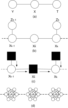
Figure 1: Comparison of the different graphical models used. (a) Gaussian Information Bottleneck [5] (b) Kalman Filter (c) Frey’s sum-product factor graph [6] (d) Our new construction.

Since the underlying graphical model of both algorithms (GIB and Kalman filter) is Markovian with Gaussian probabilities, it is interesting to ask what is the relation between them. In this work we show, that the Kalman filter posterior error covariance computation is a special case of the GIB algorithm when $\beta=1$. Furthermore, we show how to compute GIB using the Kalman filter when $\beta>1$ (the case where $0<\beta<1$ is not interesting since it gives a degenerate solution where $A_{k}\equiv 0$ [5].) Table I outlines the different notations used by both algorithms.

Theorem 2

The GIB algorithm when $\beta=1$ is equivalent to the Kalman filter algorithm.

The proof is given in Appendix B.

Theorem 3

The GIB algorithm when $\beta>1$ can be computed by a modified Kalman filter iteration.

The proof is given in Appendix C.

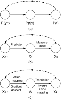
Figure 2: Comparison of the schematic operation of the different algorithms. (a) iterative information bottleneck operation (b) Kalman filter operation (c) Affine-scaling operation.

There are some differences between the GIB algorithm and Kalman filter computation. First, the Kalman filter has input observations $z_{k}$ in each round. Note that the observations do not affect the posterior error covariance computation $P_{k}$ (eq. 3c), but affect the posterior mean $\hat{x}_{k}$ (eq. 3b). Second, Kalman filter computes both posterior mean $\hat{x_{k}}$ and error covariance $P_{k}$. The covariance $\Sigma_{\xi_{k}}$ computed by the GIB algorithm was shown to be identical to $P_{k}$ when $\beta=1$. The GIB algorithm does not compute the posterior mean, but computes an additional covariance $A_{k}$ (eq. 6b), which is assumed known in the Kalman filter.

From the information theoretic perspective, our work extends the ideas presented in [10]. Predictive information is defined to be the mutual information between the past and the future of a time serias. In that sense, by using Theorem 2, Kalman filter can be thought of as a prediction of the future, which from the one hand compresses the information about past, and from the other hand maintains information about the present.

The origins of similarity between the GIB algorithm and Kalman filter are rooted in the IB iterative algorithm: For computing (5a), we need to compute (5b,5c) in recursion, and vice versa.

IV Relation to the Affine-scaling algorithm

One of the most efficient interior point methods used for linear programming is the Affine-scaling algorithm [11]. It is known that the Kalman filter is linked to the Affine-scaling algorithm [7]. In this work we give an alternate proof, based on different construction, which shows that Affine-scaling is an instance of Kalman filter, which is an instance of GIB. This link between estimation and optimization allows for numerous applications. Furthermore, by providing a single distribute efficient implementation of the GIB algorithm, we are able to solve numerous problems in communication networks.

The linear programming problem in its canonical form is given by:

minimize $${\bf c}^{T}{\bf x}$$ (7a)

subject to $$A{\bf x}={\bf b},\ \ \ \ {\bf x}\geq 0.$$ (7b)

where $A\in\mathbb{R}^{n\times p}$ with $\mathbf{rank}\{A\}=p<n$. We assume the problem is solvable with an optimal ${\bf x}^{*}$. We also assume that the problem is strictly feasible, in other words there exists ${\bf x}\in\mathbb{R}^{n}$ that satisfies $A{\bf x}={\bf b}$ and ${\bf x}>0$.

The Affine-scaling algorithm [11] is summarized below. Assume ${\bf x}_{0}$ is an interior feasible point to (7b). Let $D=diag({\bf x}_{0})$. The Affine-scaling is an iterative algorithm which computes a new feasible point that minimizes the cost function (7a):

$${\bf x}_{1}={\bf x}_{0}-\frac{\alpha}{\gamma}D^{2}{\bf r}$$ (8)

where $0<\alpha<1$ is the step size, ${\bf r}$ is the step direction.

$${\bf r} = ({\bf c}-A^{T}{\bf w}),$$ (9a)

$${\bf w} = (AD^{2}A^{T})^{-1}AD^{2}{\bf c},$$ (9b)

$$\gamma = \max_{i}({\bf e}_{i}PD{\bf c}).$$ (9c)

Where ${\bf e}_{i}$ is the $i^{th}$ unit vector and $P$ is a projection matrix given by:

$$P=I-DA^{T}(AD^{2}A^{T})^{-1}AD.$$ (10)

The algorithm continues in rounds and is guaranteed to find an optimal solution in at most $n$ rounds. In a nutshell, in each iteration, the Affine-scaling algorithm first performs an Affine-scaling with respect to the current solution point ${\bf x}_{i}$ and obtains the direction of descent by projecting the gradient of the transformed cost function on the null space of the constraints set. The new solution is obtained by translating the current solution along the direction found and then mapping the result back into the original space [7]. This has interesting analogy for the two phases of the Kalman filter.

Theorem 4

The Affine-scaling algorithm iteration is an instance of the Kalman filter algorithm iteration.

Proof is given in Appendix D.

V Efficient distributed computation

We have shown how to express the Kalman filter, Gaussian information bottleneck and Affine-scaling algorithms as a two step MMSE computation. Each step involves inverting a $2\times 2$ block matrix. Recent result by Bickson and Shental et al. [1] show that the MMSE computation can be done efficiently and distributively using the Gaussian belief propagation algorithm. Because of space limitations the full algorithm is not reproduced here.

The interested reader is referred to [3, 1] for a complete derivation of the GaBP update rules and convergence analysis. The GaBP algorithm is summarized in Table II.

TABLE II: Computing ${\bf x}={\bf A}^{-1}{\bf b}$ via GaBP [3].

# Stage Operation 1. Initialize Compute $P_{ii}=A_{ii}$ and $\mu_{ii}=b_{i}/A_{ii}$. Set $P_{ki}=0$ and $\mu_{ki}=0$, $\forall k\neq i$. 2. Iterate Propagate $P_{ki}$ and $\mu_{ki}$, $\forall k\neq i\;\mbox{\rm such that}\;A_{ki}\neq 0$. Compute $P_{i\backslash j}=P_{ii}+\sum_{{k}\in\mathbb{N}(i)\backslash j}P_{ki}$ and $\mu_{i\backslash j}=P_{i\backslash j}^{-1}(P_{ii}\mu_{ii}+\sum_{k\in\mathrm{N}(i)\backslash j}P_{ki}\mu_{ki})$. Compute $P_{ij}=-A_{ij}P_{i\backslash j}^{-1}A_{ji}$ and $\mu_{ij}=-P_{ij}^{-1}A_{ij}\mu_{i\backslash j}$. 3. Check If $P_{ij}$ and $\mu_{ij}$ did not converge, return to #2. Else, continue to #4. 4. Infer $P_{i}=P_{ii}+\sum_{{k}\in\mathrm{N}(i)}P_{ki}$ , $\mu_{i}=P_{i}^{-1}(P_{ii}\mu_{ii}+\sum_{k\in\mathrm{N}(i)}P_{ki}\mu_{ki})$. 5. Output $x_{i}=\mu_{i}$

Regarding convergence, if it converges, GaBP is known to result in exact inference [12]. Determining the exact region of convergence and convergence rate remain open research problems. All that is known is a sufficient (but not necessary) condition [13, 14] stating that GaBP converges when the spectral radius satisfies $\rho(|I_{K}-A|)<1$, where $A$ is first normalized s.t. the main diagonal contains ones. A stricter sufficient condition [12], determines that the matrix $A$ must be diagonally dominant (i.e. , $|A_{ii}|>\sum_{j\neq i}|A_{ij}|,\forall i$) in order for GaBP to converge.

Regarding convergence speed, [15] shows that when converging, the algorithm converges in $O(log(\epsilon)/log(\gamma))$ iterations, where $\epsilon$ is the desired accuracy, and $1/2<\gamma<1$ is a parameter related to the inverted matrix. The computation overhead in each iteration is determined by the number of non-zero elements of the inverted matrix $A$. In practice, [16] demonstrates convergence of 5-10 rounds on sparse matrices with several millions of variables. [17] shows convergence of dense constraint matrices of size up to $150,000\times 150,000$ in 6 rounds, where the algorithm is run in parallel using 1,024 CPUs. Empirical comparison with other iterative algorithms is given in [2].

VI Example application

The TransFab software package is a distributed middleware developed in IBM Haifa Labs, which supports real time forwarding of message streams, providing quality of service guarantees. We plan to use our distributed Kalman filter algorithm for online monitoring of software resources and performance. On each second each node records a vector of performance parameters like memory usage, CPU usage, current bandwidth, queue sizes etc. The nodes execute the distributed Kalman filter algorithm on the background. Figure 3 plots a covariance matrix of running an experiment using two TransFab nodes propagating data. The covariance matrix is used as an input the Kalman filter algorithm. Yellow sections show high correlation between measured parameters. Initial results are encouraging, we plan to report them using a future contribution.

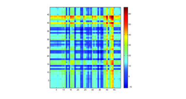
Figure 3: Covariance matrix which represents vector data captured from two Transfab nodes.

VII Conclusion

In this work we have linked together several different algorithms from the the fields of estimation (Kalman filter), clustering/compression (Gaussian information bottleneck) and optimization (Affine-scaling interior-point method). Besides of the theoretical interest in linking those different domains, we are motivated by practical problems in communication networks. To this end, we propose an efficient distributed iterative algorithm, the Gaussian belief propagation algorithm, to be used for efficiently solving these problems.

Appendix A

Proof:

We prove that inverting the matrix $E$ (eq. 4) is equivalent to one iteration of the Kalman filter for computing $P_{k}$.

We start from the matrix $E$ and show that $P_{k}^{-}$ can be computed in recursion using the Schur complement formula:

$$D-CA^{-1}B$$ (11)

applied to the $2\times 2$ upper left submatrix of E, where $D\triangleq Q,C\triangleq A^{T},B\triangleq A,A\triangleq P_{k-1}$ we get:

$$P_{k}^{-}=\overbrace{Q}^{D}\overbrace{+}^{-}\overbrace{A^{T}}^{C}\overbrace{P_{k-1}}^{-A^{-1}}\overbrace{A}^{B}.$$

Now we compute recursively the Schur complement of lower right $2\times 2$ submatrix of the matrix $E$ using the matrix inversion lemma:

$$A^{-1}+A^{-1}B(D-CA^{-1}B)^{-1}CA^{-1}$$

where $A^{-1}\triangleq P_{k}^{-},B\triangleq H^{T},C\triangleq H,D\triangleq Q.$ In total we get:

$$\overbrace{P_{k}^{-}}^{A^{-1}}+\overbrace{P_{k}^{-}}^{A^{-1}}\overbrace{H^{T}}^{B}(\overbrace{R}^{D}+\overbrace{H}^{C}\overbrace{P_{k}^{-}}^{A^{-1}}\overbrace{H^{T}}^{B})^{-1}\overbrace{H}^{C}\overbrace{P_{k}^{-}}^{A^{-1}}=$$ (12)

$$(I-\overbrace{P_{k}^{-}H^{T}(HP_{k}^{-}H^{T}+R)^{-1}}^{(\ref{kalman_gain})}H)P_{k}^{-}=$$

$$=\overbrace{(I-K_{k}H)P_{k}^{-}}^{(\ref{p_k})}=P_{k}$$

∎

Appendix B

Proof:

Looking at [5, $\S 39$], when $\beta=1$ we get

$$\begin{array}[]{l}\Sigma_{\xi+1}=(\Sigma_{t_{k}|y}^{-1})^{-1}=\Sigma_{t_{k}|y}=\\ \overbrace{\Sigma_{t_{k}}-\Sigma_{t_{k}y}\Sigma_{y}^{-1}\Sigma_{yt_{k}}}^{\mbox{MMSE}}=\\ \overbrace{\Sigma_{t_{k}}+B^{T}\Sigma_{y|t_{k}}B}^{\mbox{\cite[cite]{[\@@bibref{}{GIB}{}{}, \S 38b]}}}=\\ \Sigma_{t_{k}}+\overbrace{\Sigma_{t_{k}}^{-1}\Sigma_{t_{k}y}}^{\mbox{\cite[cite]{[\@@bibref{}{GIB}{}{}, \S 34]}}}\Sigma_{y|t_{k}}\overbrace{\Sigma_{yt_{k}}\Sigma_{t_{k}}^{-1}}^{\mbox{\cite[cite]{[\@@bibref{}{GIB}{}{}, \S 34]}}}=\\ \overbrace{A^{T}\Sigma_{x}A+\Sigma_{\xi}}^{\mbox{\cite[cite]{[\@@bibref{}{GIB}{}{}, \S 33]}}}+\overbrace{(A^{T}\Sigma_{x}A+\Sigma_{\xi})}^{\mbox{\cite[cite]{[\@@bibref{}{GIB}{}{}, \S 33]}}}A^{T}\Sigma_{xy}\cdot\\ \cdot\Sigma_{y|t_{k}}\Sigma_{yx}A\overbrace{(A^{T}\Sigma_{x}A+\Sigma_{\xi})^{T}}^{\mbox{\cite[cite]{[\@@bibref{}{GIB}{}{}, \S 33]}}}=\\ A^{T}\Sigma_{x}A+\Sigma_{\xi}+(A^{T}\Sigma_{x}A+\Sigma_{\xi})A^{T}\Sigma_{xy}\cdot\\ \cdot\overbrace{(\Sigma_{y}+\Sigma_{yt_{k}}\Sigma_{t_{k}}^{-1}\Sigma_{t_{k}y})}^{\mbox{MMSE}}\Sigma_{yx}A(A^{T}\Sigma_{x}A+\Sigma_{\xi})^{T}=\\ A^{T}\Sigma_{x}A+\Sigma_{\xi}+(A^{T}\Sigma_{x}A+\Sigma_{\xi})A^{T}\Sigma_{xy}\cdot\\ (\Sigma_{y}+\overbrace{A^{T}\Sigma_{yx}}^{\mbox{\cite[cite]{[\@@bibref{}{GIB}{}{}, \S 5]}}}\overbrace{(A\Sigma_{x}A^{T}+\Sigma_{\xi})}^{\mbox{(\cite[cite]{[\@@bibref{}{GIB}{}{}, \S 5]}}}\overbrace{\Sigma_{xy}A}^{\mbox{\cite[cite]{[\@@bibref{}{GIB}{}{}, \S 5]}}})\cdot\\ \cdot\Sigma_{yx}A(A^{T}\Sigma_{x}A+\Sigma_{\xi})^{T}.\\ \end{array}$$

Now we show this formulation is equivalent to the Kalman filter with the following notations:

$$P_{k}^{-}\triangleq(A^{T}\Sigma_{x}A+\Sigma_{\xi})\ \ ,H\triangleq A^{T}\Sigma_{yx},\ \ R\triangleq\Sigma_{y},\ \ \$$

$$P_{k-1}\triangleq\Sigma_{x},Q\triangleq\Sigma_{\xi}.$$

Substituting we get:

$$\begin{array}[]{l}\overbrace{(A^{T}\Sigma_{x}A+\Sigma_{\xi})}^{P_{k}^{-}}+\overbrace{(A^{T}\Sigma_{x}A+\Sigma_{\xi})}^{P_{k}^{-}}\overbrace{A^{T}\Sigma_{xy}}^{H^{T}}\cdot\\ \cdot(\overbrace{\Sigma_{y}}^{R}+\overbrace{A^{T}\Sigma_{yx}}^{H}\overbrace{(A^{T}\Sigma_{x}A+\Sigma_{\xi})}^{P_{k}^{-}}\overbrace{\Sigma_{xy}A}^{H^{T}})\cdot\\ \cdot\overbrace{\Sigma_{yx}A}^{H}\overbrace{(A^{T}\Sigma_{x}A+\Sigma_{\xi})}^{P_{k}^{-}}.\\ \end{array}$$

Which is equivalent to (12). Now we can apply Theorem 1 and get the desired result. ∎

Appendix C

Proof:

In the case where $\beta>1$, the MAP covariance matrix as computed by the GIB algorithm is:

$$\Sigma_{\xi_{k+1}}=\beta\Sigma_{t_{k}|y}+(1-\beta)\Sigma_{t_{k}}$$ (13)

This is a weighted average of two covariance matrices. $\Sigma_{t_{k}}$ is computed at the first phase of the algorithm (equivalent to the prediction phase in Kalman literature), and $\Sigma_{t_{k}|y}$ is computed in the second phase of the algorithm (measurement phase). At the end of the Kalman iteration, we simply compute the weighted average of the two matrices to get (13). Finally, we compute $A_{k+1}$ using (eq. 6b) by substituting the modified $\Sigma_{\xi_{k+1}}$. ∎

Appendix D

Proof:

We start by expanding the Affine-scaling update rule:

$$\begin{array}[]{c}{\bf x}_{1}=\overbrace{{\bf x}_{0}-\frac{\alpha}{\gamma}D^{2}{\bf r}}^{(\ref{af_11})}={\bf x}_{0}-\frac{\alpha}{\underbrace{\max_{i}{\bf e}_{i}PD{\bf c}}_{(\ref{af_9d})}}D^{2}{\bf r}=\\ ={\bf x}_{0}-\frac{\alpha}{\max_{i}{\bf e}_{i}\underbrace{(I-DA^{T}(AD^{2}A^{T})AD)}_{(\ref{af_10})}D{\bf c}}D^{2}{\bf r}=\\ ={\bf x}_{0}-\frac{\alpha D^{2}\overbrace{({\bf c}-A^{T}{\bf w})}^{(\ref{af_9b})}}{\max_{i}{\bf e}_{i}(I-DA^{T}(AD^{2}A^{T})^{-1}AD)D{\bf c}}=\\ {\bf x}_{0}-\frac{\alpha D^{2}({\bf c}-A^{T}\overbrace{(AD^{2}A^{T})^{-1}AD^{2}{\bf c}}^{(\ref{af_9c})})}{\max_{i}{\bf e}_{i}(I-DA^{T}(AD^{2}A^{T})AD)^{-1}D{\bf c}}=\\ {\bf x}_{0}-\frac{\alpha D(I-DA^{T}(AD^{2}A^{T})^{-1}AD)D{\bf c}}{\max_{i}{\bf e}_{i}(I-DA^{T}(AD^{2}A^{T})^{-1}AD)D{\bf c}}\\ \end{array}$$

Looking at the numerator and using the Schur complement formula (11) with the following notations: $A\triangleq(AD^{2}A^{T})^{-1},B\triangleq AD,C\triangleq DA^{T},D\triangleq I$ we get the following matrix: $\left(\begin{array}[]{cc}AD^{2}A^{T}&AD\\ DA^{T}&I\\ \end{array}\right)$. Again, the upper left block is a Schur complement $A\triangleq 0,B\triangleq AD,C\triangleq DA^{T},D\triangleq I$ of the following matrix: $\left(\begin{array}[]{cc}0&AD\\ DA^{T}&I\\ \end{array}\right)$. In total with get a $3\times 3$ block matrix of the form: $\left(\begin{array}[]{ccc}0&AD&0\\ DA^{T}&I&AD\\ 0&DA^{T}&I\\ \end{array}\right)$.
Note that the divisor is a scalar which affects the scaling of the step size.

Using Theorem 1, we get a computation of Kalman filter with the following parameters: $A,H\triangleq AD,Q\triangleq I,R\triangleq I,P_{0}\triangleq 0$. This has an interesting interpretation in the context of Kalman filter: both prediction and measurement transformation are identical and equal $AD$. The noise variance of both transformations are Gaussian variables with prior $\propto\mathcal{N}(0,I)$. ∎

References

- [1] D. Bickson, O. Shental, P. H. Siegel, J. K. Wolf, and D. Dolev, “Gaussian belief propagation based multiuser detection,” in IEEE Int. Symp. on Inform. Theory (ISIT), Toronto, Canada, July 2008.
- [2] ——, “Linear detection via belief propagation,” in Proc. 45th Allerton Conf. on Communications, Control and Computing, Monticello, IL, USA, Sept. 2007.
- [3] O. Shental, D. Bickson, P. H. Siegel, J. K. Wolf, and D. Dolev, “Gaussian belief propagation solver for systems of linear equations,” in IEEE Int. Symp. on Inform. Theory (ISIT), Toronto, Canada, July 2008.
- [4] G. Welch and G. Bishop, “An introduction to the kalman filter,” Tech. Rep., 2006. [Online]. Available: http://www.cs.unc.edu/ welch/kalman/kalmanIntro.html
- [5] G. Chechik, A. Globerson, N. Tishby, and Y. Weiss, “Information bottleneck for gaussian variables,” in Journal of Machine Learning Research, vol. 6. Cambridge, MA, USA: MIT Press, 2005, pp. 165–188.
- [6] F. Kschischang, B. Frey, and H. A. Loeliger, “Factor graphs and the sum-product algorithm,” in IEEE Transactions on Information Theory, vol. 47, Feb. 2001, pp. 498–519.
- [7] S. Puthenpura, L. Sinha, S.-C. Fang, and R. Saigal, “Solving stochastic programming problems via kalman filter and affine scaling,” in European Journal of Operational Research, vol. 83, no. 3, 1995, pp. 503–513. [Online]. Available: http://ideas.repec.org/a/eee/ejores/v83y1995i3p503-513.html
- [8] N. Tishby, F. Pereira, and W. Bialek, “The information bottleneck method,” in The 37th annual Allerton Conference on Communication, Control, and Computing, invited paper, September 1999.
- [9] N. Slonim, “The information bottelneck: Theory and application,” in Ph.D. Thesis, School of Computer Science and Enigeering, The Hebrew University of Jerusalem, 2003.
- [10] W. Bialek, I. Nemenman, and N. Tishby, “Predictability, complexity, and learning,” in Neural Comput., vol. 13, no. 11. Cambridge, MA, USA: MIT Press, November 2001, pp. 2409–2463.
- [11] R. J. Vanderbei, M. S. Meketon, and B. A. Freedman, “A modification of karmarkar’s linear programming algorithm,” in Algorithmica, vol. 1, no. 1, March 1986, pp. 395–407.
- [12] Y. Weiss and W. T. Freeman, “Correctness of belief propagation in Gaussian graphical models of arbitrary topology,” in Neural Computation, vol. 13, no. 10, 2001, pp. 2173–2200.
- [13] J. Johnson, D. Malioutov, and A. Willsky, “Walk-sum interpretation and analysis of gaussian belief propagation,” in Nineteenth Annual Conference on Neural Information Processing Systems (NIPS 05’), 2005.
- [14] D. M. Malioutov, J. K. Johnson, and A. S. Willsky, “Walk-sums and belief propagation in Gaussian graphical models,” in Journal of Machine Learning Research, vol. 7, Oct. 2006.
- [15] D. Bickson, Y. Tock, D. Dolev, and O. Shental, “Polynomial linear programming with gaussian belief propagation,” in the 46th Allerton Conf. on Communications, Control and Computing, Monticello, IL, USA, 2008.
- [16] D. Bickson and D. Malkhi, “A unifying framework for rating users and data items in peer-to-peer and social networks,” in Peer-to-Peer Networking and Applications (PPNA) Journal, Springer-Verlag, 2008.
- [17] D. Bickson, D. Dolev, and E. Yom-Tov, “A gaussian belief propagation solver for large scale support vector machines,” in 5th European Conference on Complex Systems, Jerusalem, Sept. 2008.