Interband superconductivity: contrasts between BCS and Eliashberg theory

Abstract

The newly discovered iron pnictide superconductors apparently present an unusual case of interband-channel pairing superconductivity. Here we show that, in the limit where the pairing occurs within the interband channel, several surprising effects occur quite naturally and generally: different density-of-states on the two bands lead to several unusual properties, including a gap ratio which behaves inversely to the ratio of density-of-states; the weak-coupling limit of the Eliashberg and the BCS theory, commonly taken as equivalent, in fact predict qualitatively different dependence of the $\Delta_{1}/\Delta_{2}$ and $\Delta/T_{c}$ ratios on coupling constants. We show analytically that these effects follow directly from the interband character of superconductivity. Our results show that in the interband-only pairing model the maximal gap ratio is $\sqrt{N_{2}/N_{1}}$ as strong-coupling effects act only to reduce this ratio. This suggests that if the large experimentally reported gap ratios (up to a factor 2) are correct, the pairing mechanism must include more intraband interaction than is usually assumed.

Athough first proposed 50 years ago, multiband superconductivity where the order parameter is different in different bands had not attracted much interest until 2001 when MgB₂ was found to be a two-band suprconductor. MgB₂ represents a partucular case where one “leading” band enjoys the strongest pairing interactions, while the interband pairing interaction, as well as the intraband pairing in the other band, are weak. There is growing evidence that the newly disovered superconducting ferropnictides represent another limiting case: the pairing interaction is predominantly interband, while the intraband pairing in both bands is weak. This leads to a number of interesting and qualitatively new effects, including the fact that a repulsive interband interaction is nearly as effective in creating superconductivity as an attractive one.

In this paper we will show another surprising feature of the two-band “interband” superconductivity (meaning superconductivity induced predominantly by interband interactions): entirely counterintuitively, the BCS theory for such superconductors is not the weak coupling limit of the Eliashberg theory, and the difference is not only quantitative but qualitative. This fact holds for either repulsive (as, presumably, in pnictides) or attractive interactions.

Specifically, we will concentrate on the dependence of the superconducting gaps in the two bands on the ratio of the densities of states and the magnitude of the superconducting coupling. We will show that the gap ratio is always smaller in the Eliashberg theory than in the BCS theory, the deviation grows with coupling strength and with temperature, and is largest just below $T_{c}.$

Let us start with the BCS equationsBCS . For a two band interband-only case, with gap parameters given on the two bands as $\Delta_{1}$ and $\Delta_{2}$, the BCS gap equations take the form

$$\Delta_{1} = \sum_{k}\frac{V\Delta_{2}\tanh(E_{2,k}/2k_{B}T)}{2E_{2,k}}$$

$$\Delta_{2} = \sum_{k}\frac{V\Delta_{1}(k)\tanh(E_{1,k}/2k_{B}T)}{2E_{1,k^{{}^{\prime}}}}$$ (1)

where $E_{i,k}$ is the usual quasiparticle energy in band $i$ given by $\sqrt{(\epsilon_{i,k}-\mu)^{2}+\Delta_{i}^{2}}$, the normal state electron energy is $\epsilon_{i,k},$ $\mu$ is the chemical potential. and $V$ is the interband interaction causing the superconductivity. $V$ can be either attractive ($>0$ in this convention) or repulsive (as presumably in the pnictides), but for the rest of the paper the sign does not matter. For simplicity we will use $V>0$ and $\Delta>0,$ keeping in mind that for pnictides all the results apply by substituting $\Delta$ by $|\Delta|.$ The BCS theory assumes $V$ to be constant up to the cut-off energy $\omega_{c}$. Following the BCS prescription, we can convert the momentum sums to energy integrals up to a cut-off energy $\omega_{c}$ and assume Fermi-level density-of-states (DOS) $N_{1}$ and $N_{2}.$ Near $T_{c}$ these equations can be linearized giving

$$\Delta_{1} = \Delta_{2}\lambda_{12}\log(1.136\omega_{c}/T_{c})$$

$$\Delta_{2} = \Delta_{1}\lambda_{21}\log(1.136\omega_{c}/T_{c}),$$ (2)

where $\lambda_{12}=N_{2}V$, the dimensionless coupling constant, with a similar expression for $\lambda_{21}$ . These equations readily yield $\lambda_{eff}=\sqrt{\lambda_{12}\lambda_{21}}$ and $\alpha=\Delta_{2}/\Delta_{1}=\sqrt{N_{1}/N_{2}}.$ This result has been obtained beforeparker ; bang . Similarly, at $T=0$ in the weak-coupling limit

$$\Delta_{1} = \Delta_{2}\lambda_{12}\sinh^{-1}(\omega_{c}/\Delta_{2})$$

$$\Delta_{2} = \Delta_{1}\lambda_{21}\sinh^{-1}(\omega_{c}/\Delta_{1})$$ (3)

Obviously, for $\lambda_{eff}\rightarrow 0$ we have $T_{c}\rightarrow 0$ and the relation $\Delta_{2}/\Delta_{1}=\sqrt{N_{1}/N_{2}}$ should hold. The same is not true for $\lambda_{eff}>0.$

First principle calculations suggest for the pnictides $\beta=N_{2}/N_{1}\lesssim 1.4,$ corresponding to the gap ratio $\alpha\lesssim 1.2.$ Experimental estimates for the gaps differ wildly, yielding gap ratios ranging from 1.3 to 3.4. Since the goal of this paper is to address the effect of the density of states difference on the gap ratio, we will use an intermediate numbermalone $\alpha=1.6$ ($\beta=2.6).$

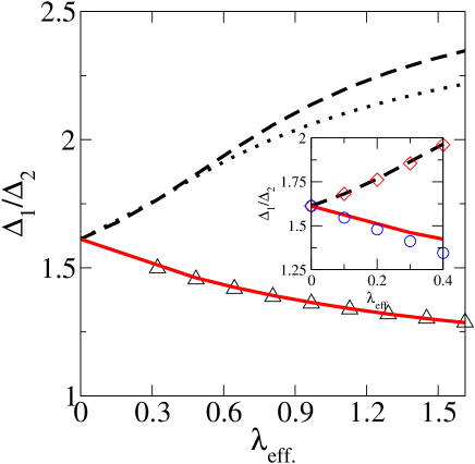
Figure 1: (color online) The ratio of the gap functions in an interband pairing case, as a function of $\lambda_{eff}$, for the BCS (dashed line) and Eliashberg Einstein (line) spectrum and spin fluctuation (triangle) spectrum cases. The dotted line represents numerical Eliashberg Einstein spectrum results in which the mass renormalization parameter has been artificially taken as 1, showing that the difference between BCS and Eliashberg is mainly a mass renormalization effect. Inset: analytic approximations to numerical results: diamonds are BCS Eq. 5, circles are Eliashberg Eq. 16.

The fact that the band with the larger DOS ends up with a smaller gap is a somewhat counterintuitive result. This is a direct result of the interband-only pairing - the pairing amplitude on one band is generated by the DOS on the other. Numerical solution of Eqs. 2 at $T=0$ (Fig. 1 gives, as expected, $\alpha=\sqrt{\beta}=1.61$ at $\lambda_{eff}\rightarrow 0.$ As a function of $\lambda_{eff}$ it increases linearly, reaching $\approx 2.3$ at $\lambda_{eff}\approx 1.6$ (note that as shown below, it will ultimately saturate at $\beta=2.6$ in the superstrong limit ). This increase can be easily explained.

Let us define $\alpha=\beta^{1/2}$, so that $x\ll 1$ at $\lambda\ll 1,$ and substitute $\sinh^{-1}(\omega_{c}/\Delta)\rightarrow\log(2\omega_{c}/\Delta).$ A few lines of algebra then lead to

$$x=\frac{\log{\beta}}{2(1+2/\sqrt{\lambda_{12}\lambda_{21}})}\simeq\frac{\lambda_{eff}\log\beta}{4}$$ (4)

This result was also obtained by Bang bang . The quadratic in $\lambda$ term can also be worked out and reads

$$\frac{\Delta_{2}}{\Delta_{1}}=\sqrt{\beta}[1+\frac{\lambda_{eff}\log\beta}{4}+\frac{\lambda_{eff}^{2}(4\log\beta+\log^{2}\beta)}{32}]$$ (5)

As Fig. 1 shows, this expression describes the numerical solution at small $\lambda$ very well. Although not apparent from the plots, the $\Delta_{1}/\Delta_{2}$ ratio will saturate at large $\lambda$, as shown by Bang and Choi bang and can also be seen from Eq. 3, since

$$\Delta_{1} = \Delta_{2}\lambda_{12}\sinh^{-1}(\omega_{c}/\Delta_{2})\rightarrow\lambda_{12}\omega_{c}\mathrm{\,\,for\,\,}\Delta_{2}\gg\omega_{c}$$ (6)

Similarly, in this limit $\Delta_{2}=\lambda_{21}\omega_{c}$ so that $\Delta_{1}/\Delta_{2}=\lambda_{12}/\lambda_{21}=N_{2}/N_{1}$. All these BCS results, however are opposite to a known analytical result GD that in the superstrong (Eliashberg) limit $\lambda\gg 1$ the gap ratio $\alpha\rightarrow 1$ independent of $\beta$. Let us now move to the strong-coupling limit, given by Eliashberg eliashberg theory.

In this theory, the BCS gap function $\Delta_{0}$ is replaced by a complex, energy-dependent quantity $\Delta_{0}(\omega)$, which must be determined along with a mass renormalization parameter $Z(\omega)$. One commonly formulates the equations in terms of $\phi(\omega)=Z(\omega)\Delta(\omega)$, and these equations can be solved either on the real frequency axis or the imaginary axis (using Matsubara frequencies). These equations are formulated in a two-band interband pairing case on the imaginary axis as follows (some of the notation is repeated from nicol ):

$$\Delta_{1}(i\omega_{n})Z_{1}(i\omega_{n}) = \pi T\sum_{m}K_{12}(i\omega_{m}-i\omega_{n})\frac{\Delta_{2}(i\omega_{m})}{\sqrt{\omega_{m}^{2}+\Delta_{2}^{2}(i\omega_{m})}}$$ (7)

$$Z_{1}(i\omega_{n}) = 1+\frac{\pi T}{\omega_{n}}\sum_{m}K_{12}(i\omega_{m}-i\omega_{n})\frac{\omega_{m}}{\sqrt{\omega_{m}^{2}+\Delta_{2}^{2}(i\omega_{m})}}$$ (8)

Here the kernel K₁₂ is given by

$$K_{12}(i\omega_{m}-i\omega_{n})=2\int_{0}^{\infty}\frac{\Omega B_{12}(\Omega)d\Omega}{\Omega^{2}+(\omega_{n}-\omega_{n})^{2}}$$

This ${B}_{12}$ represents the electron-boson coupling function which supplants the pairing potential used in BCS theory, and there is an exactly analogous equation for band 2. Here $B_{12}(\Omega)/B_{21}(\Omega)=N_{2}/N_{1}=\beta.$

First we assume a simple Einstein-type electron-boson coupling function. Numerical solution of the Eliashberg equations (8) finds that the ratio of the gaps decreases with $\lambda,$ opposite to the BCS prediction that the ratio of the gaps increases with increasing coupling. This can be understood analytically as well.

First of all, we observe that neglecting the mass renormalization by setting $Z=1$ in Eq.7 appears to be very close to the BCS solution (in fact, deviation from the lowest-order approximation of Eq. 4 is mainly due to the increasing difference between $\sinh^{-1}(\omega_{c}/\Delta)$ and $\log(2\omega_{c}/\Delta))$. Let us now work out the effect of the mass renormalization.

Assuming an Einstein spectrum with the frequency $\Omega$, at T=0 Eqs. 7,8 reduce to

$$\Delta_{1}(\omega)Z_{1}(\omega) = \frac{\lambda_{12}\Omega^{2}}{2}\int_{-\infty}^{\infty}\frac{d\omega^{{}^{\prime}}\Delta_{2}(\omega^{{}^{\prime}})}{(\Omega^{2}+(\omega-\omega^{{}^{\prime}})^{2})(\sqrt{\omega^{{}^{\prime}2}+\Delta_{2}^{2}(\omega)})}$$

and

$$Z_{1}(\omega) = 1+\frac{1}{2\omega}\lambda_{12}\Omega^{2}\int_{-\infty}^{\infty}d\omega^{`}\frac{\omega^{{}^{\prime}}}{(\Omega^{2}+(\omega-\omega^{{}^{\prime}})^{2})(\sqrt{\omega^{{}^{\prime}2}+\Delta_{2}^{2}(\omega)})}$$

with a similar equation for $\Delta_{2}$ and Z₂. In the popular “square-well” approximationSW ; pm the equations become

$$\Delta_{1}(\omega)Z_{1}(\omega) = \frac{\lambda_{12}\theta(\Omega-|\omega|)}{2}\int_{-\infty}^{\infty}d\omega^{{}^{\prime}}\times$$

$$\theta(\Omega-|\omega^{{}^{\prime}})|\frac{\Delta_{2}(\omega^{{}^{\prime}})}{(\Omega^{2}+(\omega-\omega^{{}^{\prime}})^{2})(\sqrt{\omega^{{}^{\prime}2}+\Delta_{2}^{2}})}$$

$$Z_{1}(\omega) = 1+\frac{1}{2\omega}\lambda_{12}\int_{-\infty}^{\infty}d\omega^{{}^{\prime}}\theta(\Omega-|\omega-\omega^{{}^{\prime}}|)\times$$ (10)

$$\frac{\Delta_{2}(\omega^{{}^{\prime}})}{(\Omega^{2}+(\omega-\omega^{{}^{\prime}})^{2})(\sqrt{\omega^{{}^{\prime}2}+\Delta_{2}^{2}})}$$

which may be readily integrated to yield the following renormalization behavior for $Z(\omega)$:

$$Z_{1}(\omega) = 1+\lambda_{12}\mathrm{\,\,for\,\,}\omega<\Omega$$ (11)

$$= 1+\lambda_{12}\Omega/\omega\mathrm{\,\,for\,\,}\Omega<\omega<2\Omega$$ (12)

$$= 1+\lambda_{12}/2\mathrm{\,\,for\,\,}\omega>2\Omega$$ (13)

This mass renormalization behavior can then be incorporated in the previous BCS equations yielding a natural result:

$$\Delta_{1}(1+\lambda_{12}) = \Delta_{2}\lambda_{12}\sinh^{-1}(\omega_{c}/\Delta_{2})$$ (14)

$$\Delta_{2}(1+\lambda_{21}) = \Delta_{1}\lambda_{21}\sinh^{-1}(\omega_{c}/\Delta_{1}),$$ (15)

reducing to Eq. 3 with $\lambda_{12}\rightarrow\lambda_{12}/(1+\lambda_{12}),\lambda_{21}\rightarrow\lambda_{21}/(1+\lambda_{21}).$ Thus, in the linear order in $\lambda.$

$$\frac{\Delta_{2}}{\Delta_{1}}=\sqrt{\beta}(1+\frac{\lambda_{eff}\log\beta}{4}+\frac{\lambda_{21}-\lambda_{12}}{2})$$ (16)

The last term is negative and always larger than the previous one (independent of $\beta).$ Thus, the net effect is always opposite to what the BCS theory predicts. We have plotted up the above analytic approximation in Figure 1 (solid line in inset) and find good agreement for $\lambda_{eff}<0.4$, showing that the mass renormalization is responsible for the lessening of the gap ratios with increasing coupling in Eliashberg theory. This result might in hindsight have been expected given that the Fermi surface with the larger gap at weak-coupling can be expected to have larger self-energy interactions in Eliashberg theory, reducing the gap anisotropy. This result is also consistent with the superstrong coupling limit of equal gaps, as mentioned previously.

Interestingly, this strong coupling effect remains operative at all temperatures up to $T_{c},$ while the previous term in Eq. 16 vanishes at $T_{c}.$ Therefore (cf. Fig.2) the actual gap ratio is even closer to 1 near $T_{c}$ than at $T=0.$

Finally, we note that the above Eliashberg results were obtained using an Einstein spectral function for simplicity, but as indicated on the plot the use of a typical spin-fluctuation spectrum ${[\sim\omega\Omega/(}\omega^{2}+\Omega^{2}{)]}$ does not alter the results.

Another interesting observation to be made concerns the $\Delta(0)/T_{c}$ ratios predicted by BCS and Eliashberg theory. In the conventional weak-coupling one-band BCS theory this ratio does not depend on $\lambda.$ This is no longer the case in the two-band BCS with the interband coupling only.  In the lowest order the reduced gaps are simply $\Delta_{1}(0)/T_{c}=1.76\beta^{1/4},$ $\Delta_{2}(0)/T_{c}=1.76\beta^{-1/4}.$ The next order can be worked out using Eq. 5:

$$\frac{\Delta_{1}(0)}{T_{c}} = 1.76\beta^{1/4}(1+\lambda\frac{4\log\beta-\log^{2}\beta}{32})$$ (17)

$$\frac{\Delta_{2}(0)}{T_{c}} = 1.76\beta^{-1/4}(1-\lambda\frac{4\log\beta+\log^{2}\beta}{32})$$ (18)

This is confirmed by numerical calculations (Fig. 2): the smaller gap ratio decreases with $\lambda,$ while the other gap increases.

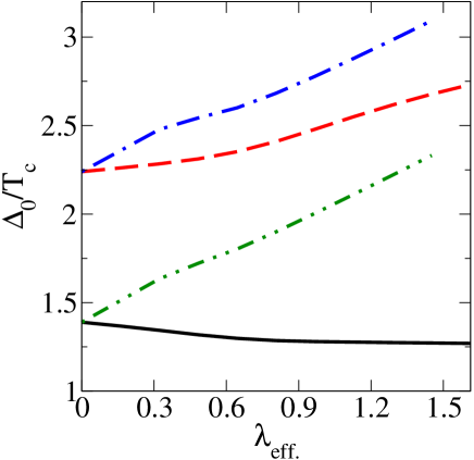
Figure 2: (color online) $\Delta(T=0)/T_{c}$ ratios are shown, as a function of the overall coupling constant, for the BCS (solid black line and gray dashed line) and Eliashberg (dot-dashed line and double-dot-dashed line) cases.

Since the Eliashberg equation makes the gaps closer with increased coupling, this odd behavior does not show up: both reduced gaps grow with $\lambda.$

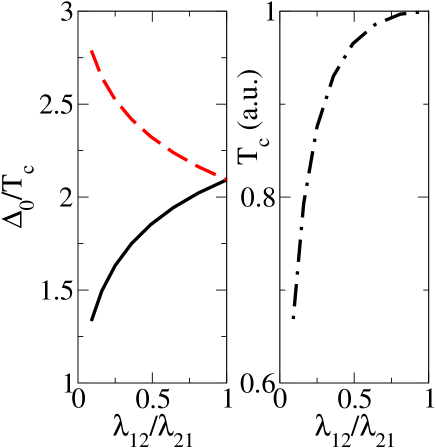
Figure 3: (color online). (left) The behavior of the Eliashberg $\Delta(0)/T_{c}$ ratios as a function of the ratio of coupling constants. (right) The behavior of T_c in this case. For both cases $\lambda_{\mathrm{eff}}$ is fixed at 1.

For completeness, we also show in Fig. 3 the behavior (in Eliashberg theory) of the reduced gaps as a function of the DOS ratio $N_{2}/N_{1}=$$\lambda_{12}/\lambda_{21}$. As might be expected, as the DOS ratio becomes very small the gap ratios move apart appreciably. Interestingly, ${T}$_c (shown in the right panel) is not constant as it would be in a weak-coupling regime, but varies significantly for coupling constant ratios far from 1. This is a result of the use of comparatively large coupling constants on one band when the other coupling constant is small, so that $T_{c}$ suppression due to thermal excitation of real phonons (an effect not present in the BCS formalism) is stronger.

To conclude, in this work we have shown for the interband-only pairing the two-band superconductivity is qualitatively incorrectly described by the BCS formalism even for the weak coupling limit. BCS and Eliashberg theory predict qualitatively different behavior (as a function of coupling constant) for such basic characteristics as the gap ratio $\alpha=\Delta_{1}/\Delta_{2},$ as well as for the reduced gaps $\Delta/T_{c}$. In particular, the sign of $d\alpha/d\lambda$ changes from BCS to Eliashberg theory.  We have found this result analytically and numerically, by solving Eliashberg equations for model spectra. This finding is relevant to the superconducting pnictides where the interband-pairing regime is believed to be realized.

References

(1) J.R. Schrieffer, Theory of superconductivity,
(Reading:Perseus), 1999.
(2) D. Parker, O. Dolgov, M.M. Korshunov, A. Golubov and
I.I. Mazin, accepted for publication in Physical Review B, 2008.
(3) Y. Bang and H.-Y. Choi, arXiv:0807.3912 (unpublished).
(4) L. Malone, J.D. Fletcher, A. Serafin, A. Carrington,
N.D. Zhigadlo, Z. Bukowksi, S. Katrych and J. Karpinski, arXiv:0806.3908
(unpublished).
(5) O.V. Dolgov and A.A. Golubov, Phys. Rev B 77 214526
(2008).
(7) E.J. Nicol and J.P. Carbotte, Phys. Rev. B 71,
054501 (2005).
(8) P.B. Allen and B. Mitrovic, Sol. State Phys. 37, 1
(1982).
(9) The square well model is not a consistent approximation, as different
functional forms are assumed for in the first and in the second
Eliashberg equation. Sometimes this may lead to qualitative errors (O.V.
Dolgov et al, : Phys. Rev. Lett. 95, 257003, 2005). In
this particular case, however, it can be shown that using more accurate
and consistent functional forms, and leads to essentially the same result.