Discontinuous Galerkin Methods for the Helmholtz Equation with Large Wave Number

Abstract

This paper develops and analyzes some interior penalty discontinuous Galerkin methods using piecewise linear polynomials for the Helmholtz equation with the first order absorbing boundary condition in the two and three dimensions. It is proved that the proposed discontinuous Galerkin methods are stable (hence well-posed) without any mesh constraint. For each fixed wave number $k$, optimal order (with respect to $h$) error estimate in the broken $H^{1}$-norm and sub-optimal order estimate in the $L^{2}$-norm are derived without any mesh constraint. The latter estimate improves to optimal order when the mesh size $h$ is restricted to the preasymptotic regime (i.e., $k^{2}h\gtrsim 1$). Numerical experiments are also presented to gauge the theoretical result and to numerically examine the pollution effect (with respect to $k$) in the error bounds. The novelties of the proposed interior penalty discontinuous Galerkin methods include: first, the methods penalize not only the jumps of the function values across the element edges but also the jumps of the normal and tangential derivatives; second, the penalty parameters are taken as complex numbers of positive imaginary parts so essentially and practically no constraint is imposed on the penalty parameters. Since the Helmholtz problem is a non-Hermitian and indefinite linear problem, as expected, the crucial and the most difficult part of the whole analysis is to establish the stability estimates (i.e., a priori estimates) for the numerical solutions. To the end, the cruxes of our analysis are to establish and to make use of a local version of the Rellich identity (for the Laplacian) and to mimic the stability analysis for the PDE solutions given in [23, 24, 35].

1 Introduction

Wave is ubiquitous, it arises in many branches of science, engineering and industry (cf. [22, 39] and the references therein). It is significant to geoscience, petroleum engineering, telecommunication, and defense industry. Mathematically, wave propagation problems are described by hyperbolic partial differential equations, and the progress of solving wave-related application problems has largely depended on the progress of developing effective methods and algorithms to solve their governing partial differential equations. Among many wave-related application problems, those dealing with high frequencies (or large wave numbers) wave propagation are most difficult to solve numerically because they are strongly indefinite and non-Hermitian and their solutions are very oscillatory. These properties in turn make it very difficult to construct stable numerical schemes under practical mesh constraints. Furthermore, high frequency (or large wave number) requires to use very fine meshes in order to resolve highly oscillatory waves, and the use of fine meshes inevitably gives rise huge, strongly indefinite, ill-conditioned, and non-Hermitian (algebraic) systems to solve. All these difficulties associated with high frequency (large wave number) wave computation still remain to be resolved and are not mathematically well understood in high dimensions (cf. [49]), although considerable amount of progresses have been made in the past thirty years (cf. [29, 36, 39] and the references therein).

The simplest prototype wave scattering problem is the following acoustic scattering problem (with time dependence $e^{{\rm\mathbf{i}}\omega t}$):

(1) $$-\Delta u-k^{2}u =f\qquad \mbox{in }\mathbf{R}^{d}\setminus D,$$

(2) $$u =0 \mbox{on }\partial D,$$

(3) $$\sqrt{r}\Bigl{(}\frac{\partial(u-u^{\rm inc})}{\partial r}+{\rm\mathbf{i}}k(u-u^{\rm inc})\Bigr{)} \rightarrow 0 \mbox{as }r=|x|\rightarrow\infty,$$

where $D\subset\mathbf{R}^{d}\,(d=2,3)$, a bounded Lipschitz domain, denotes the scatterer and ${\rm\mathbf{i}}=\sqrt{-1}$ denotes the imaginary unit. $k\in\mathbf{R}$ is a given positive (large) number and known as the wave number. $u^{\rm inc}$ is the incident wave. Equation (1) is the well-known Helmholtz equation and condition (3) is the Sommerfeld radiation condition at the infinity. Boundary condition (2) implies that the scatterer is sound-soft.

To compute the solution of the above problem, due to (finite) memory and speed limitations of computers, one needs first to formulate the problem as a finite domain problem. Two major approaches have been developed for the task in the past thirty years. The first approach is boundary integral methods (cf. [48] and the references therein) and the other one is artificial boundary condition methods (cf. [28, 13] and the references therein). In the case of boundary integral methods, one converts the original differential equation into a (complicate) boundary integral equation on the boundary $\partial D$ of the scatterer $D$. Clearly, the trade-off is that the original simple differential equation could not be retained in the conversion. On the other hand, artificial boundary condition methods solve the given differential equation on a truncated computational domain by imposing suitable artificial boundary conditions on the outer boundary of the computational domain. Artificial boundary condition methods can be divided into two groups. One group of the methods use sharp artificial boundaries (i.e., the boundary has zero width), appropriate boundary conditions, which are called “absorbing boundary conditions”, then are imposed on the boundaries (cf. [28, 30]). The second group of artificial boundary condition methods allow the artificial boundaries to have non-zero width, such fatten boundaries are called absorbing layers, where the artificial boundary conditions are usually constructed in the form of differential equations which replace the original wave equations in the absorbing layers. The methods of this second group are called “PML (perfectly matched layer) methods” (cf. [13]). In this paper, we shall adopt the absorbing boundary condition approach for problem (1)–(3). Extension of the results of this paper to the PML formulations will be given elsewhere.

Specifically, in this paper we consider the following Helmholtz problem:

(4) $$-\Delta u-k^{2}u =f \qquad\mbox{in }\Omega:=\Omega_{1}\setminus D,$$

(5) $$u =0 \qquad\mbox{on }\Gamma_{D},$$

(6) $$\frac{\partial u}{\partial n_{\Omega}}+{\rm\mathbf{i}}ku =g \qquad\mbox{on }\Gamma_{R},$$

where $(D\subset)\,\Omega_{1}\subset\mathbf{R}^{d},\,d=2,3$ is a polygonal/polyhedral domain, which is often taken as a $d$-rectangle in applications. $\Gamma_{R}:=\partial\Omega_{1},\Gamma_{D}=\partial D$, hence, $\partial\Omega=\Gamma_{R}\cup\Gamma_{D}$. $n_{\Omega}$ denotes the unit outward normal to $\partial\Omega$. The Robin boundary condition (6) is known as the first order absorbing boundary condition (cf. [28]). We remark that the case $D=\emptyset$ also arises in applications either as a consequence of frequency domain treatment of waves or when time-harmonic solutions of the scalar wave equation are sought (cf. [26, 27]).

For many years, the finite element method (and other type methods) has been widely used to discretize the Helmholtz equation (4) with various types of boundary conditions (cf. [1, 2, 5, 6, 12, 16, 21, 23, 27, 29, 33, 37, 36, 39, 42] and the reference therein). It is well known that in every coordinate direction, one must put some minimal number of grid points in each wave length $\ell=2\pi/k$ in order to resolve the wave, that is, the mesh size $h$ must satisfy the constraint $hk\lesssim 1$. In practice, $6-10$ grid points are used in a wave length, which is often referred as the “rule of thumb”. However, this “rule of thumb” was proved rigorously not long ago by Babuška et al [37] only in the one-dimensional case (called the preasymptotic error analysis). The main difficulty of the analysis is caused by the strong indefiniteness of the Helmholtz equation which in turn makes it hard to establish stability estimates for the finite element solution under the “rule of thumb” mesh constraint. In [37], Babuška et al also showed that the $H^{1}$-error bound for the finite element solution contains a pollution term that is related to the loss of stability with large wave numbers. Later, Babuška et al addressed the question whether it is possible to reduce the pollution effect in a series of papers (cf. Chapter 4 of [36] and the reference therein). It should be noted that under the stronger mesh condition that $k^{2}h$ is sufficiently small, optimal (with respect to $h$) and quasi-optimal (with respect to $k$) error estimates for finite element approximations of the Helmholtz problem were established early by Aziz and Kellogg in [5] and Douglas, et al in [26, 27] using the so-called Schatz argument [44] (also see Chapter 5 of [14]), and a similar result was also obtained in [33] using an operator perturbation argument.

The work of [5, 26, 37] shows that in the $1$-d case, due to the pollution effect, the finite element solution for the Helmholtz problem (4)-(5) deteriorates as the wave number becomes large if the practical mesh condition $kh\lesssim 1$ is used. The situation in the high dimensions is expected to be the same (at least not better) although, to the best of our knowledge, no such a rigorous analysis is known in the literature. The detailed analysis of [26, 37] also shows that the pollution effect is inherent in the finite element method and is caused by the deterioration of stability of the Helmholtz operator as the wave number $k$ becomes large. In order to minimize or eliminate (if possible) the pollution and to obtain more stable and more accurate approximate solutions for Helmholtz-type problems with large wave numbers, various nonstandard and generalized Galerkin methods have been proposed lately in the literature. These methods can be categorized into two groups. The first group of methods use nonstandard or stabilized discrete variational forms to approximate the Helmholtz operator so that the resulted discrete problems have better stability properties. Methods in this group include Galerkin-least-squares finite element methods [15, 34], quasi-stabilized finite element methods [10], and discontinuous Galerkin methods [1, 17, 38]. The second group of methods abandon the use of piecewise polynomial trial and test functions and replace them by global polynomials or non-polynomial functions. Methods in this group include spectral methods [45], generalized Galerkin/finite element methods [40, 8], partition of unity finite element methods [41], and meshless methods [8]. We also note that another very different and intensively studied approach for high frequency wave computation is geometrical optics, which studies asymptotic (nonlinear) approximations of the Helmholtz equation obtained when the frequency (or wave number) tends infinity. We refer the reader to [29] and the references therein for some recent developments in geometrical optics and its variants.

The goal of this paper is to develop some interior penalty discontinuous Galerkin (IPDG) methods for problem (4)–(5) in high dimensions. The focus of the paper is to establish the rigorous stability and error analysis, in particular, the preasymptotic error analysis. For the ease of presentation and to better present ideas, we confine ourselves to only consider the case of linear element in this paper. Such a restriction is also due to the consideration that we shall present $hp$-discontinuous Galerkin methods for problem (4)–(5) in a forth coming paper [32] which extends the work of this paper to high order elements. Compared with existing DG methods for the Helmholtz equation in the literature, the novelties of our interior penalty discontinuous Galerkin methods include the following: First, our mesh-dependent sesquilinear forms penalize not only the jumps of the function values across the element edges/faces but also the jumps of the normal and tangential derivatives. Recall that penalizing the jumps of the normal (and tangential) derivatives helps but is not essential for the success of IPDG methods in the case of coercive elliptic problems (cf. [3, 25]), however, it contributes critically to the stability of the IPDG methods of this paper. Second, a small but vitally important idea of this paper is to take the penalty parameters as complex numbers of positive imaginary parts. This idea also contributes critically to the stability of the IPDG methods of this paper. As a result, essentially and practically no constraint is imposed on the penalty parameters. Since the Helmholtz problem is a non-Hermitian and an indefinite linear problem, as expected, the crucial and the most difficult part of the whole analysis is to establish the stability estimates (i.e., a priori estimates) for the numerical solutions. To the end, the cruxes of our analysis are to establish and to make use of a local version of the Rellich identity (for the Laplacian) and to mimic the stability analysis for the PDE solutions given in [23, 24, 35]. Suppose $\Omega_{1}$ is star-shaped with respect to a point $x_{\Omega_{1}}$. The key idea is to use the special test function $\nabla u_{h}\cdot(x-x_{\Omega_{1}})$ (defined element-wise), which is a valid candidate for any IPDG method. We remark that the same technique was successfully employed by Shen and Wang in [45] to carry out the stability and error analysis for the spectral Galerkin approximation of the Helmholtz problem.

In the past fifteen years, DG methods have received a lot attentions and undergone intensive studies by many people. As is well known now, DG methods have several advantages over other types of numerical methods. For example, the trial and test spaces are very easy to construct, they can naturally handle inhomogeneous boundary conditions and curved boundaries; they also allow the use of highly nonuniform and unstructured meshes, and have built-in parallelism which permits coarse-grain parallelization. In addition, the fact that the mass matrices are block diagonal is an attractive feature in the context of time-dependent problems, especially if explicit time discretizations are used. We refer to [3, 4, 11, 19, 20, 25, 31, 46, 43, 47] and the references therein for a detailed account on DG methods for coercive elliptic and parabolic problems. In addition to the advantages listed above, the results of this paper also demonstrate the flexibility and effectiveness of DG methods for strongly indefinite problems, which was not well understood before.

The remainder of this paper is organized as follows. In Section 2, notation and some preliminaries are described and cited. In particular, the sharp (with respect to $k$) stability constant estimates of [24] for the solution of problem (4)–(5) in high dimensions were recalled. These estimates are critical for obtaining explicit dependence of the error bounds on the wave number $k$. In Section 3, the IPDG methods of this paper are formulated. Both symmetric and non-symmetric IPDG methods are constructed. However, since the Helmholtz equation and its solution are complex-valued, the non-symmetric terms in the IPDG sesquilinear form do not cancel each other when two arguments of the form are taken to be the same function. Instead, their difference is a pure imaginary quantity. This is a main difference between non-symmetric IPDG for coercive elliptic problems and for indefinite Helmholtz type problems. As a result, the penalty parameters need to be chosen as complex numbers with positive imaginary parts to ensure the stability in both symmetric and non-symmetric IPDG methods. Section 4 devotes to stability analysis for the IPDG methods proposed in Section 3. It is proved that the proposed IPDG methods are stable (hence well-posed) without any mesh constraint. In Section 5, using the stability result of Section 4 we derive optimal order (with respect to $h$) error estimate in the broken $H^{1}$-norm and sub-optimal order estimate in the $L^{2}$-norm without any mesh constraint. The latter estimate improves to optimal order when the mesh size $h$ is restricted to the preasymptotic regime (i.e., $k^{2}h\gtrsim 1$). In particular, for appropriately chosen penalty parameters, it is shown that the error in the broken $H^{1}$-norm is bounded by $\widetilde{C}_{1}kh+\widetilde{C}_{2}k^{8/3}h^{4/3}$ if $kh\lesssim 1$. Numerical tests in Section 6 suggest that the error in the broken $H^{1}$-norm may have a better bound $\widetilde{C}_{1}kh+\widetilde{C}_{2}k^{3}h^{2}$ and it is possible to tune the penalty parameters to significantly reduce the pollution error. We note that in the case $k^{2}h$ is sufficiently small, optimal order (with respect to $h$) error estimate in the broken $H^{1}$-norm can be derived by using the Schatz argument as done in [38, 5, 26, 27]. In Section 6, we present some numerical experiments to gauge our theoretical error estimates, to numerically examine the pollution effect in the error bounds, and to test the performance of the proposed IPDG methods.

2 Notation and Preliminaries

The standard space, norm and inner product notation are adopted. Their definitions can be found in [14, 18, 11]. In particular, $(\cdot,\cdot)_{Q}$ and $\langle\cdot,\cdot\rangle_{\Sigma}$ for $\Sigma\subset\partial Q$ denote the $L^{2}$-inner product on complex-valued $L^{2}(Q)$ and $L^{2}(\Sigma)$ spaces, respectively. $(\cdot,\cdot):=(\cdot,\cdot)_{\Omega}$ and $\langle\cdot,\cdot\rangle:=\langle\cdot,\cdot\rangle_{\partial\Omega}$. Let

$$H_{\Gamma_{D}}^{1}(\Omega):=\left\{u\in H^{1}(\Omega):u=0\text{ on }\Gamma_{D}\right\}.$$

Throughout the paper, $C$ is used to denote a generic positive constant which is independent of $h$ and $k$. We also use the shorthand notation $A\lesssim B$ and $B\gtrsim A$ for the inequality $A\leq CB$ and $B\geq CA$. $A\simeq B$ is a shorthand notation for the statement $A\lesssim B$ and $B\lesssim A$.

We now recall the definition of star-shaped domains.

Definition 1.

$Q\subset\mathbf{R}^{d}$ is said to be a star-shaped domain with respect to $x_{Q}\in Q$ if there exists a nonnegative constant $c_{Q}$ such that

(7) $$(x-x_{Q})\cdot n_{Q}\geq c_{Q}\qquad\forall x\in\partial Q.$$

$Q\subset\mathbf{R}^{d}$ is said to be strictly star-shaped if $c_{Q}$ is positive.

Throughout this paper, we assume that $\Omega_{1}$ is a strictly star-shaped domain. In practice, $\Omega_{1}$ is often taken as a $d$-rectangle, which trivially is a strictly star-shaped domain. We also assume the scatterer $D$ is a star-shaped domain with respect to the same point $x_{\Omega_{1}}$ as $\Omega_{1}$ does. This then implies that $x_{\Omega_{1}}\in D\subset\Omega_{1}$. More precisely, we assume that there exist constants $c_{\Omega_{1}}>0$ and $c_{D}\geq 0$ such that

(8) $$(x-x_{\Omega_{1}})\cdot n_{\Omega}\geq c_{\Omega_{1}}\quad\forall x\in\Gamma_{R}\quad\text{ and }\quad(x-x_{\Omega_{1}})\cdot n_{D}\geq c_{D}\quad\forall x\in\Gamma_{D}.$$

Here $n_{\Omega}$ and $n_{D}$ are the unit outward normals to the boundaries of $\Omega$ and $D$, respectively.

Under these assumptions the following stability estimates for problem (4)–(5) were proved in [23, 24, 35].

Theorem 2.

Suppose $\Omega_{1}\subset\mathbf{R}^{d}$ is a strictly star-shaped domain and $D\subset\Omega_{1}$ is a star-shaped domain. Then the solution $u$ to problem (4)–(5) satisfies

(9) $$\|u\|_{H^{j}(\Omega)}\lesssim\Bigl{(}\frac{1}{k}+k^{j-1}\Bigr{)}\bigl{(}\|f\|_{L^{2}(\Omega)}+\|g\|_{L^{2}(\Gamma_{R})}\bigr{)}$$

for $j=0,1$ if $u\in H^{3/2+\varepsilon}(\Omega)$ for some $\varepsilon>0$. (2.3) also holds for $j=2$ if $u\in H^{2}(\Omega).$

3 Formulation of discontinuous Galerkin methods

To formulate our IPDG methods, we first need to introduce some notation. Let $\mathcal{T}_{h}$ be a family of triangulations of the domain $\Omega:=\Omega_{1}\setminus D$ parameterized by $h>0$. For any triangle/tetrahedron $K\in\mathcal{T}_{h}$, we define $h_{K}:=\mbox{diam}(K)$. Similarly, for each edge/face $e$ of $K\in\mathcal{T}_{h}$, define $h_{e}:=\mbox{diam}(e)$. We assume that the elements of $\mathcal{T}_{h}$ satisfy the minimal angle condition. We define

$$\mathcal{E}_{h}^{I} := \mbox{ set of all interior edges/faces of $\mathcal{T}_{h}$},$$

$$\mathcal{E}_{h}^{R} := \mbox{ set of all boundary edges/faces of $\mathcal{T}_{h}$ on $\Gamma_{R}$},$$

$$\mathcal{E}_{h}^{D} := \mbox{ set of all boundary edges/faces of $\mathcal{T}_{h}$ on $\Gamma_{D}$},$$

$$\mathcal{E}_{h}^{RD} := \mathcal{E}_{h}^{R}\cup\mathcal{E}_{h}^{D}=\mbox{ set of all boundary edges/faces of $\mathcal{T}_{h}$},$$

$$\mathcal{E}_{h}^{ID} := \mathcal{E}_{h}^{I}\cup\mathcal{E}_{h}^{D}=\mbox{ set of all edges/faces of $\mathcal{T}_{h}$ except those on $\Gamma_{R}$}.$$

We also define the jump $[v]$ of $v$ on an interior edge/face $e=\partial K\cap\partial K^{\prime}$ as

$$[v]|_{e}:=\left\{\begin{array}[]{ll}v|_{K}-v|_{K^{\prime}},&\quad\mbox{if the global label of $K$ is bigger},\\ v|_{K^{\prime}}-v|_{K},&\quad\mbox{if the global label of $K^{\prime}$ is bigger}.\end{array}\right.$$

If $e\in\mathcal{E}_{h}^{D}$, set $[v]|_{e}=v|_{e}$. The following convention is adopted in this paper

$$\{v\}|_{e}:=\frac{1}{2}\bigl{(}v|_{K}+v|_{K^{\prime}}\bigr{)}\qquad\mbox{if }e=\partial K\cap\partial K^{\prime}.$$

If $e\in\mathcal{E}_{h}^{D}$, set $\{v\}|_{e}=v|_{e}$. For every $e=\partial K\cap\partial K^{\prime}\in\mathcal{E}_{h}^{I}$, let $n_{e}$ be the unit outward normal to edge/face $e$ of the element $K$ if the global label of $K$ is bigger and of the element $K^{\prime}$ if the other way around. For every $e\in\mathcal{E}_{h}^{RD}$, let $n_{e}=n_{\Omega}$ the unit outward normal to $\partial\Omega$.

Now we define the “energy” space $E$ and the sesquilinear form $a_{h}(\cdot,\cdot)$ on $E\times E$ as follows:

$$E :=\prod_{K\in\mathcal{T}_{h}}H^{2}(K),$$

(10) $$a_{h}(u,v) :=b_{h}(u,v)+{\rm\mathbf{i}}\bigl{(}J_{0}(u,v)+J_{1}(u,v)+L_{1}(u,v)\bigr{)}\qquad\forall\,u,v\in E,$$

where

(11) $$b_{h}(u,v):= \sum_{K\in\mathcal{T}_{h}}(\nabla u,\nabla v)_{K}-\sum_{e\in\mathcal{E}_{h}^{ID}}\left(\left\langle\left\{\frac{\partial u}{\partial n_{e}}\right\},\left[v\right]\right\rangle_{e}+\sigma\left\langle\left[u\right],\left\{\frac{\partial v}{\partial n_{e}}\right\}\right\rangle_{e}\right),$$

(12) $$J_{0}(u,v):= \sum_{e\in\mathcal{E}_{h}^{ID}}\frac{\gamma_{0,e}}{h_{e}}\left\langle\left[u\right],\left[v\right]\right\rangle_{e},$$

(13) $$J_{1}(u,v):= \sum_{e\in\mathcal{E}_{h}^{I}}\gamma_{1,e}h_{e}\left\langle\left[\frac{\partial u}{\partial n_{e}}\right],\left[\frac{\partial v}{\partial n_{e}}\right]\right\rangle_{e},$$

(14) $$L_{1}(u,v):= \sum_{e\in\mathcal{E}_{h}^{ID}}\sum_{j=1}^{d-1}\frac{\beta_{1,e}}{h_{e}}\left\langle\left[\frac{\partial u}{\partial\tau_{e}^{j}}\right],\left[\frac{\partial v}{\partial\tau_{e}^{j}}\right]\right\rangle_{e},$$

and $\sigma$ is an $h$-independent real number. $\gamma_{0,e},\gamma_{1,e}$, and $\beta_{1,e}$ are nonnegative numbers to be specified later. $\{\tau^{j}_{e}\}_{j=1}^{d-1}$ denote an orthogonal coordinate frame on the edge/face $e\in\mathcal{E}_{h}$, and $\frac{\partial u}{\partial\tau_{e}^{j}}:=\nabla u\cdot\tau_{e}^{j}$ stands for the tangential derivative of $u$ in the direction $\tau_{e}^{j}$.

Remark 3.1.

(a) Clearly, $a_{h}(\cdot,\cdot)$ is a consistent discretization for $-\Delta$ since $(-\Delta u,v)=a_{h}(u,v)$ for all $u\in H_{\Gamma_{D}}^{1}(\Omega)\cap H^{2}(\Omega)$ and $v\in E$.

(b) If we regard $a_{h}(\cdot,\cdot)$ as a bilinear form on the subspace of real valued functions in $H_{\Gamma_{D}}^{1}(\Omega)$, then $a_{h}(\cdot,\cdot)$ is symmetric when $\sigma=1$ and is non-symmetric when $\sigma\neq 1$. In particular, $\sigma=-1$ would correspond to the non-symmetric IPDG method studied in [46, 43] for coercive elliptic problems. In this paper, for the ease of presentation, we only consider the case $\sigma=1$, nevertheless the main results of the paper can also be extended to the case $\sigma\neq 1$.

(c) The terms in ${\rm\mathbf{i}}\bigl{(}J_{0}(u,v)+J_{1}(u,v)+L_{1}(u,v)\bigr{)}$ are so-called penalty terms.

(d) The penalty parameters in ${\rm\mathbf{i}}\bigl{(}J_{0}(u,v)+J_{1}(u,v)+L_{1}(u,v)\bigr{)}$ are ${\rm\mathbf{i}}\gamma_{0,e},{\rm\mathbf{i}}\gamma_{1,e}$ and ${\rm\mathbf{i}}\beta_{1,e}$, respectively. So they are pure imaginary numbers with positive imaginary parts. It turns out that if any of them is replaced by a complex number with positive imaginary part, the ideas of the paper still apply. Here we set their real parts to be zero partly because the terms from real parts do not help much (and do not cause any problem either) in our theoretical analysis and partly for the ease of presentation. On the other hand, our numerical experiments in Section 6.5 indicate that using penalty parameters with nonzero real parts helps to reduce the pollution effect in the error.

(e) Penalizing the jumps of normal derivatives (i.e., the $J_{1}$ term above) for second order PDEs was used early by Douglas and Dupont [25] in the context of $C^{0}$ finite element methods, by Baker [11] (with a different weighting, also see [31]) for fourth order PDEs, and by Arnold [3] in the context of IPDG methods for second order parabolic PDEs. Arnold [3] also proposed and analyzed IPDG methods which penalize higher order normal derivatives. Note that we do not introduce boundary terms for $e\in\mathcal{E}_{h}^{D}$ in $J_{1}$ to ensure the consistency of $a_{h}(\cdot,\cdot)$ with $-\Delta$.

On the other hand, the idea of penalizing the jumps of tangential derivatives (i.e., the $L_{1}$ term above) seems is new. Later we will show that without $L_{1}$ term and $J_{1}$ term in $a_{h}(\cdot,\cdot)$ the IPDG methods of this paper are still stable and convergent but under a stinger mesh constraint, see Section 4 and 5.

(f) In this paper we consider the scattering problem with time dependence $e^{{\rm\mathbf{i}}\omega t}$, that is, the signs before ${\rm\mathbf{i}}$’s in the Sommerfeld radiation condition (3) and its first order approximation (6) are positive. If we consider the scattering problem with time dependence $e^{-{\rm\mathbf{i}}\omega t}$, that is, the signs before ${\rm\mathbf{i}}$’s in (3) and (6) are negative, then the penalty parameters should be complex numbers with negative imaginary parts.

Next, we introduce the following semi-norms/norms on the space $E$:

(15) $$\bigl{|}v\bigr{|}_{1,h}:= \Big{(}\sum_{K\in\mathcal{T}_{h}}\left\|\nabla v\right\|_{L^{2}(K)}^{2}\Big{)}^{\frac{1}{2}},$$

(16) $$\left\|v\right\|_{1,h}:= \left(\bigl{|}v\bigr{|}_{1,h}^{2}+\sum_{e\in\mathcal{E}_{h}^{I}}\gamma_{1,e}h_{e}\left\|\left[\frac{\partial v}{\partial n_{e}}\right]\right\|_{L^{2}(e)}^{2}\right.$$

$$\hskip 36.135pt\left.+\sum_{e\in\mathcal{E}_{h}^{ID}}\left(\frac{\gamma_{0,e}}{h_{e}}\left\|\left[v\right]\right\|_{L^{2}(e)}^{2}+\sum_{j=1}^{d-1}\frac{\beta_{1,e}}{h_{e}}\left\|\left[\frac{\partial v}{\partial\tau_{e}^{j}}\right]\right\|_{L^{2}(e)}^{2}\right)\right)^{\frac{1}{2}},$$

(17) $$\left\|{\hskip-3.0pt}\left|v\right|{\hskip-3.0pt}\right\|_{1,h}:= \left(\left\|v\right\|_{1,h}^{2}+\sum_{e\in\mathcal{E}_{h}^{ID}}\frac{h_{e}}{\gamma_{0,e}}\left\|\left\{\frac{\partial v}{\partial n_{e}}\right\}\right\|_{L^{2}(e)}^{2}\right)^{\frac{1}{2}}.$$

It is easy to see that $\left\|\cdot\right\|_{1,h}$ and $\left\|{\hskip-3.0pt}\left|\cdot\right|{\hskip-3.0pt}\right\|_{1,h}$ are norms on $E$ if $\partial D\neq\emptyset$ but only semi-norms if $\partial D=\emptyset$.

Clearly, the sesquilinear form $a_{h}(\cdot,\cdot)$ with $\sigma=1$ satisfies: For any $v\in E$

(18) $$\operatorname{{Re}}a_{h}(v,v) =\bigl{|}v\bigr{|}_{1,h}^{2}-2\operatorname{{Re}}\sum_{e\in\mathcal{E}_{h}^{ID}}\left\langle\left\{\frac{\partial v}{\partial n_{e}}\right\},\left[v\right]\right\rangle_{e},$$

(19) $$\operatorname{{Im}}a_{h}(v,v) =J_{0}(v,v)+J_{1}(v,v)+L_{1}(v,v).$$

With the help of the sesquilinear form $a_{h}(\cdot,\cdot)$ we now introduce the following weak formulation for (4)–(5): Find $u\in E\cap H_{\Gamma_{D}}^{1}(\Omega)\cap H^{2}_{{\rm loc}}(\Omega)$ such that

(20) $$a_{h}(u,v)-k^{2}(u,v)+{\rm\mathbf{i}}k\langle u,v\rangle_{\Gamma_{R}}=(f,v)+\left\langle g,v\right\rangle_{\Gamma_{R}},\qquad\forall v\in E\cap H_{\Gamma_{D}}^{1}(\Omega)\cap H^{2}_{{\rm loc}}(\Omega).$$

The above formulation is consistent with the boundary value problem (4)–(6) because $a_{h}(\cdot,\cdot)$ is consistent with $-\Delta$. It is clear that, if $u\in H^{2}(\Omega)$ is the solution of (4)–(5), then (20) holds for all $v\in E.$

For any $K\in\mathcal{T}_{h}$, let $P_{1}(K)$ denote the set of all linear polynomials on $K$. We define our IPDG approximation space $V^{h}$ as

$$V^{h}:=\prod_{K\in\mathcal{T}_{h}}P_{1}(K).$$

Clearly, $V^{h}\subset E\subset L^{2}(\Omega)$. But $V^{h}\not\subset H^{1}(\Omega)$.

We are now ready to define our IPDG methods based on the weak formulation (20): Find $u_{h}\in V^{h}$ such that

(21) $$a_{h}(u_{h},v_{h})-k^{2}(u_{h},v_{h})+{\rm\mathbf{i}}k\langle u_{h},v_{h}\rangle_{\Gamma_{R}}=(f,v_{h})+\left\langle g,v_{h}\right\rangle_{\Gamma_{R}}\qquad\forall v_{h}\in V^{h}.$$

In the next two sections, we shall study the stability and error analysis for the above IPDG methods. Especially, we are interested in knowing how the stability constants and error constants depend on the wave number $k$ (and mesh size $h$, of course) and what are the “optimal” relationship between mesh size $h$ and the wave number $k$.

4 Stability estimates

Since the Helmholtz operator is not a coercive elliptic operator, the stability estimates given in Theorem 2 for the solution of problem (4)–(6) is far from trivial. We refer the reader to [23, 24, 35] for a detailed exposition in this direction. This difficulty is certainly inherited by any numerical discretization of problem (4)–(6). In fact, the situation usually is worse in the discrete case because piecewise polynomials (or piecewise smooth functions) are rigid, they are not as flexible as the PDE trial functions. On the other hand, DG approximation functions are much more flexible than Lagrange finite element functions because they do not have any continuity constraint, instead, the continuity of the numerical solutions is enforced weakly through mesh-dependent bilinear or sesquilinear or nonlinear forms.

The goal of this section is to derive stability estimates (or a priori estimates) for scheme (21). To the end, momentarily, we assume solution $u_{h}$ to (21) exists and will revisit the existence and uniqueness issues later at the end of the section. We like to note that because its strong indefiniteness, unlike in the case of coercive elliptic and parabolic problems (cf. [3, 4, 11, 25, 31, 46, 43, 47]), the well-posedness of scheme (21) is far from obvious under practical mesh constraints.

To derive stability estimates for scheme (21), our approach is to mimic the stability analysis for the Helmholtz problem (4)–(6) given in [23, 24, 35]. It turns out that this approach indeed works for scheme (21) although the analysis is more delicate and complicate than that for the differential problem. The key ingredients of our analysis are to use a special test function $v_{h}=\alpha\cdot{\rm NewA}u_{h}$ (defined element-wise) with $\alpha(x):=x-x_{\Omega_{1}}$ in (21) and to use the Rellich identity (cf. [24] and below) on each element.

Our first lemma of this section establishes three integral identities which play an important role in our analysis.

Lemma 3.

Let $\alpha(x):=x-x_{\Omega_{1}}$, $v\in E$, $K\in\mathcal{T}_{h}$ and $e\in\mathcal{E}_{h}^{ID}$. Then there hold

(22) $$d\left\|v\right\|_{L^{2}(K)}^{2}+2\operatorname{{Re}}(v,\alpha\cdot{\rm NewA}v)_{K}=\int_{\partial K}\alpha\cdot n_{K}\bigl{|}v\bigr{|}^{2},$$

(23) $$(d-2)\left\|{\rm NewA}v\right\|_{L^{2}(K)}^{2}+2\operatorname{{Re}}\big{(}{\rm NewA}v,{\rm NewA}(\alpha\cdot{\rm NewA}v)\big{)}_{K}=\int_{\partial K}\alpha\cdot n_{K}\bigl{|}{\rm NewA}v\bigr{|}^{2},$$

(24) $$\left\langle\left\{\frac{\partial v}{\partial n_{e}}\right\},\left[\alpha\cdot{\rm NewA}v\right]\right\rangle_{e}-\left\langle\alpha\cdot n_{e}\left\{{\rm NewA}v\right\},\left[{\rm NewA}v\right]\right\rangle_{e}$$

$$\hskip 97.56493pt=\sum_{j=1}^{d-1}\int_{e}\left(\alpha\cdot\tau_{e}^{j}\left\{\frac{\partial v}{\partial n_{e}}\right\}-\alpha\cdot n_{e}\left\{\frac{\partial v}{\partial\tau_{e}^{j}}\right\}\right)\frac{\partial\left[\overline{v}\right]}{\partial\tau_{e}^{j}},$$

where $x_{\Omega_{1}}$ denotes the point in the star-shaped domain definition for $\Omega_{1}$ (see (8)). Also note that in (22) and (23), we omit the sign ds in the integrals. We shall adopt this omission consistently throughout this paper to save space.

Proof.

It is easy to verify by direct computations the following differential identities on $K$:

$$\mathrm{div}(\alpha(x)) \equiv d,$$

$$\mathrm{div}(\alpha v\overline{v}) =dv\overline{v}+(\alpha\cdot{\rm NewA}v)\overline{v}+v(\alpha\cdot{\rm NewA}\overline{v}),$$

$$\mathrm{div}(\alpha({\rm NewA}v\cdot{\rm NewA}\overline{v})) =(d-2){\rm NewA}v\cdot{\rm NewA}\overline{v}+{\rm NewA}(\alpha\cdot{\rm NewA}v)\cdot{\rm NewA}\overline{v}+{\rm NewA}v\cdot{\rm NewA}(\alpha\cdot{\rm NewA}\overline{v}).$$

(22) and (23) then follows immediately from integrating the above second and third identities over $K$.

To prove identity (24), from the representations

$${\rm NewA}v=\frac{\partial v}{\partial n_{e}}n_{e}+\sum_{j=1}^{d-1}\frac{\partial v}{\partial\tau_{e}^{j}}\tau_{e}^{j},\hskip 36.135pt\alpha\cdot{\rm NewA}v=\frac{\partial v}{\partial n_{e}}\alpha\cdot n_{e}+\sum_{j=1}^{d-1}\frac{\partial v}{\partial\tau_{e}^{j}}\alpha\cdot\tau_{e}^{j},$$

we have

$$\left\langle\left\{\frac{\partial v}{\partial n_{e}}\right\},\left[\alpha\cdot{\rm NewA}v\right]\right\rangle_{e}-\left\langle\alpha\cdot n_{e}\left\{{\rm NewA}v\right\},\left[{\rm NewA}v\right]\right\rangle_{e}$$

$$\hskip 43.36243pt=\int_{e}\left(\alpha\cdot n_{e}\left\{\frac{\partial v}{\partial n_{e}}\right\}\left[\frac{\partial\overline{v}}{\partial n_{e}}\right]+\sum_{j=1}^{d-1}\alpha\cdot\tau_{e}^{j}\left\{\frac{\partial v}{\partial n_{e}}\right\}\left[\frac{\partial\overline{v}}{\partial\tau_{e}^{j}}\right]\right)$$

$$\hskip 72.26999pt-\int_{e}\left(\alpha\cdot n_{e}\left\{\frac{\partial v}{\partial n_{e}}\right\}\left[\frac{\partial\overline{v}}{\partial n_{e}}\right]+\alpha\cdot n_{e}\sum_{j=1}^{d-1}\left\{\frac{\partial v}{\partial\tau_{e}^{j}}\right\}\left[\frac{\partial\overline{v}}{\partial\tau_{e}^{j}}\right]\right)$$

$$\hskip 43.36243pt=\sum_{j=1}^{d-1}\int_{e}\left(\alpha\cdot\tau_{e}^{j}\left\{\frac{\partial v}{\partial n_{e}}\right\}-\alpha\cdot n_{e}\left\{\frac{\partial v}{\partial\tau_{e}^{j}}\right\}\right)\frac{\partial\left[\overline{v}\right]}{\partial\tau_{e}^{j}},$$

which completes the proof of the lemma. ∎

Remark 4.1.

The identity (23) can be viewed as a local version of the Rellich identity for the Laplacian $\Delta$ (cf. [23, 24]). Since $V^{h}\subset E$, hence, (22)–(24) also hold for any function $v=v_{h}\in V^{h}$.

Now, taking $v_{h}=u_{h}$ in (21) yields

(25) $$a_{h}(u_{h},u_{h})-k^{2}\left\|u_{h}\right\|_{L^{2}(\Omega)}^{2}+{\rm\mathbf{i}}k\left\|u_{h}\right\|_{L^{2}(\Gamma_{R})}^{2}=(f,u_{h})+\left\langle g,u_{h}\right\rangle_{\Gamma_{R}}.$$

Therefore, taking real part and imaginary part of the above equation and using (18) and (19) we get the following lemma.

Lemma 4.

Let $u_{h}\in V^{h}$ solve (21). Then

(26) $$\bigl{|}u_{h}\bigr{|}_{1,h}^{2}-2\operatorname{{Re}}\sum_{e\in\mathcal{E}_{h}^{ID}}\left\langle\left\{\frac{\partial u_{h}}{\partial n_{e}}\right\},\left[u_{h}\right]\right\rangle_{e}-k^{2}\left\|u_{h}\right\|_{L^{2}(\Omega)}^{2}\leq\bigl{|}(f,u_{h})+\left\langle g,u_{h}\right\rangle_{\Gamma_{R}}\bigr{|},$$

(27) $$\sum_{e\in\mathcal{E}_{h}^{ID}}\left(\frac{\gamma_{0,e}}{h_{e}}\left\|\left[u_{h}\right]\right\|_{L^{2}(e)}^{2}+\sum_{j=1}^{d-1}\frac{\beta_{1,e}}{h_{e}}\left\|\left[\frac{\partial u_{h}}{\partial\tau_{e}^{j}}\right]\right\|_{L^{2}(e)}^{2}\right)+\sum_{e\in\mathcal{E}_{h}^{I}}\gamma_{1,e}h_{e}\left\|\left[\frac{\partial u_{h}}{\partial n_{e}}\right]\right\|_{L^{2}(e)}^{2}$$

$$\hskip 195.12877pt+k\left\|u_{h}\right\|_{L^{2}(\Gamma_{R})}^{2}\leq\bigl{|}(f,u_{h})+\left\langle g,u_{h}\right\rangle_{\Gamma_{R}}\bigr{|}.$$

From (26) and (27) we can easily bound $\bigl{|}u_{h}\bigr{|}_{1,h}$ and the jumps in terms of $\left\|u_{h}\right\|_{L^{2}(\Omega)}$. In order to get the desired a priori estimates, we now need to derive a reverse inequality whose coefficient on the right-hand side can be controlled. Such a reverse inequality, which is often difficult to get under practical mesh constraints, and stability estimates for scheme (21) will be derived next.

Theorem 5.

Let $u_{h}\in V^{h}$ solve (21) and suppose $\gamma_{0,e},\gamma_{1,e},\beta_{1,e}>0$. Define $M(f,g):=\left\|f\right\|_{L^{2}(\Omega)}+\|g\|_{L^{2}(\Gamma_{R})}$. Then there exists a positive constant $C_{\rm sta}$ such that

(28) $$\left\|u_{h}\right\|_{L^{2}(\Omega)} +\frac{1}{k}\left\|u_{h}\right\|_{1,h}+\frac{1}{k}\Bigl{(}\sum_{e\in\mathcal{E}_{h}^{R}}\left\|{\rm NewA}u_{h}\right\|_{L^{2}(e)}^{2}\Bigr{)}^{\frac{1}{2}}$$

$$+\frac{1}{k}\Bigl{(}\sum_{e\in\mathcal{E}_{h}^{D}}c_{D}\bigl{(}k^{2}\left\|u_{h}\right\|_{L^{2}(e)}^{2}+\left\|{\rm NewA}u_{h}\right\|_{L^{2}(e)}^{2}\bigr{)}\Bigr{)}^{\frac{1}{2}}\lesssim C_{\rm sta}\,M(f,g)$$

and

(29) $$C_{\rm sta} \leq\frac{1}{k}+\frac{1}{k^{2}}+\frac{1}{k^{2}}\max_{e\in\mathcal{E}_{h}^{D}}\left(\frac{1}{\gamma_{0,e}}+\frac{\gamma_{0,e}}{h_{e}}+\sqrt{\frac{\gamma_{0,e}}{\beta_{1,e}}}+\frac{1}{\beta_{1,e}}\right)$$

$$\qquad\qquad\;\;+\frac{1}{k^{2}}\max_{e\in\mathcal{E}_{h}^{I}}\left(\frac{k^{2}+1}{\gamma_{0,e}}+\frac{1}{h_{e}}\sqrt{\frac{\gamma_{0,e}}{\gamma_{1,e}}}+\sqrt{\frac{\gamma_{0,e}}{\beta_{1,e}}}+\frac{1}{\beta_{1,e}}\right).$$

Proof.

Since the proof is long, we divide it into three steps.

Step 1: A representation identity for $\left\|u_{h}\right\|_{L^{2}(\Omega)}$. It follows from (22) with $v=u_{h}$ that

$$d\left\|u_{h}\right\|_{L^{2}(K)}^{2}=\int_{\partial K}\alpha\cdot n_{K}\bigl{|}u_{h}\bigr{|}^{2}-2\operatorname{{Re}}(u_{h},\alpha\cdot\nabla u_{h})_{K}.$$

Summing over all $K\in\mathcal{T}_{h}$ yields

$$d\left\|u_{h}\right\|_{L^{2}(\Omega)}^{2}=\sum_{K\in\mathcal{T}_{h}}\int_{\partial K}\alpha\cdot n_{K}\bigl{|}u_{h}\bigr{|}^{2}-2\sum_{K\in\mathcal{T}_{h}}\operatorname{{Re}}(u_{h},\alpha\cdot\nabla u_{h})_{K},$$

hence,

(30) $$2k^{2}\left\|u_{h}\right\|_{L^{2}(\Omega)}^{2}=k^{2}\sum_{K\in\mathcal{T}_{h}}\int_{\partial K}\alpha\cdot n_{K}\bigl{|}u_{h}\bigr{|}^{2}-(d-2)k^{2}\left\|u_{h}\right\|_{L^{2}(\Omega)}^{2}-2k^{2}\operatorname{{Re}}(u_{h},v_{h}),$$

where $v_{h}\in E$ is defined by $v_{h}|_{K}=\alpha\cdot{\rm NewA}u_{h}|_{K}$ for every $K\in\mathcal{T}_{h}$. It is easy to check that $v_{h}|_{K}$ is a linear polynomial on $K$, hence, $v_{h}\in V^{h}$. Using this $v_{h}$ as a test function in (21) and taking the real part of the resulted equation we get

(31) $$-k^{2}\operatorname{{Re}}(u_{h},v_{h})=\operatorname{{Re}}\bigl{(}(f,v_{h})+\left\langle g,v_{h}\right\rangle_{\Gamma_{R}}-a_{h}(u_{h},v_{h})-{\rm\mathbf{i}}k\left\langle u_{h},v_{h}\right\rangle_{\Gamma_{R}}\bigr{)}.$$

Now, it follows from (30), (25) and (31) that

$$2k^{2}\left\|u_{h}\right\|_{L^{2}(\Omega)}^{2} =k^{2}\sum_{K\in\mathcal{T}_{h}}\int_{\partial K}\alpha\cdot n_{K}\bigl{|}u_{h}\bigr{|}^{2}+(d-2)\operatorname{{Re}}\bigl{(}(f,u_{h})+\left\langle g,u_{h}\right\rangle_{\Gamma_{R}}-a_{h}(u_{h},u_{h})\bigr{)}$$

$$\quad+2\operatorname{{Re}}\bigl{(}(f,v_{h})+\left\langle g,v_{h}\right\rangle_{\Gamma_{R}}-a_{h}(u_{h},v_{h})-{\rm\mathbf{i}}k\left\langle u_{h},v_{h}\right\rangle_{\Gamma_{R}}\bigr{)}$$

$$=k^{2}\sum_{K\in\mathcal{T}_{h}}\int_{\partial K}\alpha\cdot n_{K}\bigl{|}u_{h}\bigr{|}^{2}+(d-2)\operatorname{{Re}}\bigl{(}(f,u_{h})+\left\langle g,u_{h}\right\rangle_{\Gamma_{R}}\bigr{)}$$

(32) $$\quad+2\operatorname{{Re}}\bigl{(}(f,v_{h})+\left\langle g,v_{h}\right\rangle_{\Gamma_{R}}\bigr{)}+2k\operatorname{{Im}}\left\langle u_{h},v_{h}\right\rangle_{\Gamma_{R}}$$

$$\quad-\sum_{K\in\mathcal{T}_{h}}\left((d-2)\left\|{\rm NewA}u_{h}\right\|_{L^{2}(K)}^{2}+2\operatorname{{Re}}({\rm NewA}u_{h},{\rm NewA}v_{h})_{K}\right)$$

$$\quad+2\sum_{e\in\mathcal{E}_{h}^{ID}}\left((d-2)\operatorname{{Re}}\left\langle\left\{\frac{\partial u_{h}}{\partial n_{e}}\right\},\left[u_{h}\right]\right\rangle_{e}+\operatorname{{Re}}\left\langle\left\{\frac{\partial u_{h}}{\partial n_{e}}\right\},\left[v_{h}\right]\right\rangle_{e}\right.$$

$$\quad\left.+\operatorname{{Re}}\left\langle\left[u_{h}\right],\left\{\frac{\partial v_{h}}{\partial n_{e}}\right\}\right\rangle_{e}\right)+2\operatorname{{Im}}\big{(}J_{0}(u_{h},v_{h})+J_{1}(u_{h},v_{h})+L_{1}(u_{h},v_{h})\big{)}.$$

Using the identity $\bigl{|}a\bigr{|}^{2}-\bigl{|}b\bigr{|}^{2}=\operatorname{{Re}}(a+b)(\bar{a}-\bar{b})$ we have

(33) $$\sum_{K\in\mathcal{T}_{h}}\int_{\partial K}\alpha\cdot n_{K}\bigl{|}u_{h}\bigr{|}^{2}=2\sum_{e\in\mathcal{E}_{h}^{I}}\operatorname{{Re}}\left\langle\alpha\cdot n_{e}\left\{u_{h}\right\},\left[u_{h}\right]\right\rangle_{e}+\left\langle\alpha\cdot n_{\Omega},|u_{h}|^{2}\right\rangle_{\partial\Omega}.$$

From the Rellich identity (23) and noting that $\left\langle\alpha\cdot n_{e}\left\{{\rm NewA}u_{h}\right\},\left[{\rm NewA}u_{h}\right]\right\rangle_{e}=\left\langle\alpha\cdot n_{e},|{\rm NewA}u_{h}|^{2}\right\rangle_{e}$ for $e\in\mathcal{E}_{h}^{D}$ we get

(34) $$\sum_{K\in\mathcal{T}_{h}}\Bigl{(}(d-2)\left\|{\rm NewA}u_{h}\right\|_{L^{2}(K)}^{2}+2\operatorname{{Re}}({\rm NewA}u_{h},{\rm NewA}v_{h})_{K}\Bigr{)}=\sum_{K\in\mathcal{T}_{h}}\int_{\partial K}\alpha\cdot n_{K}\bigl{|}{\rm NewA}u_{h}\bigr{|}^{2}$$

$$= 2\sum_{e\in\mathcal{E}_{h}^{I}}\operatorname{{Re}}\left\langle\alpha\cdot n_{e}\left\{{\rm NewA}u_{h}\right\},\left[{\rm NewA}u_{h}\right]\right\rangle_{e}+\sum_{e\in\mathcal{E}_{h}^{RD}}\left\langle\alpha\cdot n_{e},|{\rm NewA}u_{h}|^{2}\right\rangle_{e}.$$

$$= 2\sum_{e\in\mathcal{E}_{h}^{ID}}\operatorname{{Re}}\left\langle\alpha\cdot n_{e}\left\{{\rm NewA}u_{h}\right\},\left[{\rm NewA}u_{h}\right]\right\rangle_{e}+\sum_{e\in\mathcal{E}_{h}^{R}}\left\langle\alpha\cdot n_{e},|{\rm NewA}u_{h}|^{2}\right\rangle_{e}-\sum_{e\in\mathcal{E}_{h}^{D}}\left\langle\alpha\cdot n_{e},|{\rm NewA}u_{h}|^{2}\right\rangle_{e}.$$

On noting that $u_{h}$ is piecewise linear and $v_{h}|_{K}=(x-x_{\Omega_{1}})\cdot{\rm NewA}u_{h}|_{K}$, then ${\rm NewA}v_{h}|_{K}={\rm NewA}u_{h}|_{K}$. Hence,

(35) $$\operatorname{{Im}}\big{(}J_{1}(u_{h},v_{h})+L_{1}(u_{h},v_{h})\big{)}=\operatorname{{Im}}\big{(}J_{1}(u_{h},u_{h})+L_{1}(u_{h},u_{h})\big{)}=0.$$

Plugging (33)–(35) into (32) then gives the following representation for $\left\|u_{h}\right\|_{L^{2}(\Omega)}$:

$$2k^{2}\left\|u_{h}\right\|_{L^{2}(\Omega)}^{2} =(d-2)\operatorname{{Re}}\bigl{(}(f,u_{h})+\left\langle g,u_{h}\right\rangle_{\Gamma_{R}}\bigr{)}+2\operatorname{{Re}}\bigl{(}(f,v_{h})+\left\langle g,v_{h}\right\rangle_{\Gamma_{R}}\bigr{)}$$

$$\quad+2k^{2}\sum_{e\in\mathcal{E}_{h}^{I}}\operatorname{{Re}}\left\langle\alpha\cdot n_{e}\left\{u_{h}\right\},\left[u_{h}\right]\right\rangle_{e}+k^{2}\left\langle\alpha\cdot n_{\Omega},|u_{h}|^{2}\right\rangle_{\partial\Omega}$$

$$\quad+2k\operatorname{{Im}}\left\langle u_{h},v_{h}\right\rangle_{\Gamma_{R}}-\sum_{e\in\mathcal{E}_{h}^{R}}\left\langle\alpha\cdot n_{e},|{\rm NewA}u_{h}|^{2}\right\rangle_{e}+\sum_{e\in\mathcal{E}_{h}^{D}}\left\langle\alpha\cdot n_{e},|{\rm NewA}u_{h}|^{2}\right\rangle_{e}$$

(36) $$\quad+2\sum_{e\in\mathcal{E}_{h}^{ID}}\operatorname{{Re}}\left(-\left\langle\alpha\cdot n_{e}\left\{{\rm NewA}u_{h}\right\},\left[{\rm NewA}u_{h}\right]\right\rangle_{e}+\left\langle\left\{\frac{\partial u_{h}}{\partial n_{e}}\right\},\left[v_{h}\right]\right\rangle_{e}\right)$$

$$\quad+2\sum_{e\in\mathcal{E}_{h}^{ID}}\left((d-1)\operatorname{{Re}}\left\langle\left\{\frac{\partial u_{h}}{\partial n_{e}}\right\},\left[u_{h}\right]\right\rangle_{e}+\operatorname{{Re}}\left\langle\left[u_{h}\right],\left\{\frac{\partial v_{h}}{\partial n_{e}}\right\}\right\rangle_{e}\right)$$

$$\quad-2\sum_{e\in\mathcal{E}_{h}^{ID}}\operatorname{{Re}}\left\langle\left\{\frac{\partial u_{h}}{\partial n_{e}}\right\},\left[u_{h}\right]\right\rangle_{e}+2\operatorname{{Im}}J_{0}(u_{h},v_{h}).$$

Step 2: Derivation of a reverse inequality. We bound each terms on the right hand side of (4). For an edge/face $e\in\mathcal{E}_{h}^{I}$, let $K_{e}$ and $K_{e}^{\prime}$ denote the two elements in $\mathcal{T}_{h}$ that share $e$. For an edge/face $e\in\mathcal{E}_{h}^{D}$, let $K_{e}$ denote the element in $\mathcal{T}_{h}$ that has $e$ as an edge/face and $K_{e}^{\prime}=\emptyset$. We have

(37) $$2k^{2}\sum_{e\in\mathcal{E}_{h}^{I}}\operatorname{{Re}}\left\langle\alpha\cdot n_{e}\left\{u_{h}\right\},\left[u_{h}\right]\right\rangle_{e} \leq Ck^{2}\sum_{e\in\mathcal{E}_{h}^{I}}h_{e}^{-\frac{1}{2}}\left\|u_{h}\right\|_{L^{2}(K_{e}\cup K_{e}^{\prime})}\left\|\left[u_{h}\right]\right\|_{L^{2}(e)}$$

$$\leq\frac{k^{2}}{3}\left\|u_{h}\right\|_{L^{2}(\Omega)}^{2}+C\sum_{e\in\mathcal{E}_{h}^{I}}\frac{k^{2}}{\gamma_{0,e}}\frac{\gamma_{0,e}}{h_{e}}\left\|\left[u_{h}\right]\right\|_{L^{2}(e)}^{2}.$$

It is clear that

(38) $$k^{2}\left\langle\alpha\cdot n_{\Omega},|u_{h}|^{2}\right\rangle_{\partial\Omega} =k^{2}\left\langle\alpha\cdot n_{\Omega},|u_{h}|^{2}\right\rangle_{\Gamma_{R}}+\sum_{e\in\mathcal{E}_{h}^{D}}k^{2}\left\langle\alpha\cdot n_{e},|u_{h}|^{2}\right\rangle_{e}$$

$$\leq Ck^{2}\left\|u_{h}\right\|_{L^{2}(\Gamma_{R})}^{2}+\sum_{e\in\mathcal{E}_{h}^{D}}k^{2}\left\langle\alpha\cdot n_{e},|u_{h}|^{2}\right\rangle_{e}.$$

It follows from the star-shaped assumption on $\Omega_{1}$ that

(39) $$2k \operatorname{{Im}}\left\langle u_{h},v_{h}\right\rangle_{\Gamma_{R}}-\sum_{e\in\mathcal{E}_{h}^{R}}\left\langle\alpha\cdot n_{e},|{\rm NewA}u_{h}|^{2}\right\rangle_{e}$$

$$\leq Ck\sum_{e\in\mathcal{E}_{h}^{R}}\left\|u_{h}\right\|_{L^{2}(e)}\left\|{\rm NewA}u_{h}\right\|_{L^{2}(e)}-c_{\Omega_{1}}\sum_{e\in\mathcal{E}_{h}^{R}}\left\|{\rm NewA}u_{h}\right\|_{L^{2}(e)}^{2}$$

$$\leq Ck^{2}\left\|u_{h}\right\|_{L^{2}(\Gamma_{R})}^{2}-\frac{c_{\Omega_{1}}}{2}\sum_{e\in\mathcal{E}_{h}^{R}}\left\|{\rm NewA}u_{h}\right\|_{L^{2}(e)}^{2}.$$

By (24) we obtain

(40) $$2\sum_{e\in\mathcal{E}_{h}^{ID}}\operatorname{{Re}}\left(-\left\langle\alpha\cdot n_{e}\left\{{\rm NewA}u_{h}\right\},\left[{\rm NewA}u_{h}\right]\right\rangle_{e}+\left\langle\left\{\frac{\partial u_{h}}{\partial n_{e}}\right\},\left[v_{h}\right]\right\rangle_{e}\right)$$

$$\hskip 36.135pt=2\sum_{e\in\mathcal{E}_{h}^{ID}}\sum_{j=1}^{d-1}\operatorname{{Re}}\int_{e}\left(\alpha\cdot\tau_{e}^{j}\left\{\frac{\partial u_{h}}{\partial n_{e}}\right\}-\alpha\cdot n_{e}\left\{\frac{\partial u_{h}}{\partial\tau_{e}^{j}}\right\}\right)\frac{\partial\left[\overline{u}_{h}\right]}{\partial\tau_{e}^{j}}$$

$$\hskip 36.135pt\lesssim\sum_{e\in\mathcal{E}_{h}^{ID}}\sum_{j=1}^{d-1}h_{e}^{-\frac{1}{2}}\sum_{K=K_{e},K_{e}^{\prime}}\left\|{\rm NewA}u_{h}\right\|_{L^{2}(K)}\left\|\left[\frac{\partial u_{h}}{\partial\tau_{e}^{j}}\right]\right\|_{L^{2}(e)}$$

$$\hskip 36.135pt\leq\frac{1}{3}\bigl{|}u_{h}\bigr{|}_{1,h}^{2}+C\sum_{e\in\mathcal{E}_{h}^{ID}}\frac{1}{\beta_{1,e}}\sum_{j=1}^{d-1}\frac{\beta_{1,e}}{h_{e}}\left\|\left[\frac{\partial u_{h}}{\partial\tau_{e}^{j}}\right]\right\|_{L^{2}(e)}^{2}.$$

Noting that $\frac{\partial v_{h}}{\partial n_{e}}=\frac{\partial u_{h}}{\partial n_{e}}$ we have

(41) $$2\sum_{e\in\mathcal{E}_{h}^{ID}}\left((d-1)\operatorname{{Re}}\left\langle\left\{\frac{\partial u_{h}}{\partial n_{e}}\right\},\left[u_{h}\right]\right\rangle_{e}+\operatorname{{Re}}\left\langle\left[u_{h}\right],\left\{\frac{\partial v_{h}}{\partial n_{e}}\right\}\right\rangle_{e}\right)$$

$$\hskip 36.135pt\lesssim\sum_{e\in\mathcal{E}_{h}^{ID}}h_{e}^{-\frac{1}{2}}\sum_{K=K_{e},K_{e}^{\prime}}\left\|{\rm NewA}u_{h}\right\|_{L^{2}(K)}\left\|\left[u_{h}\right]\right\|_{L^{2}(e)}$$

$$\hskip 36.135pt\leq\frac{1}{3}\bigl{|}u_{h}\bigr{|}_{1,h}^{2}+C\sum_{e\in\mathcal{E}_{h}^{ID}}\frac{1}{\gamma_{0,e}}\frac{\gamma_{0,e}}{h_{e}}\left\|\left[u_{h}\right]\right\|_{L^{2}(e)}^{2}.$$

From (12), the inverse inequality and (27) we get

(42) $$2\operatorname{{Im}}\big{(} J_{0}(u_{h},v_{h})\big{)}=2\operatorname{{Im}}\sum_{e\in\mathcal{E}_{h}^{ID}}\frac{\gamma_{0,e}}{h_{e}}\left\langle\left[u_{h}\right],\left[v_{h}\right]\right\rangle_{e}$$

$$=2\operatorname{{Im}}\sum_{e\in\mathcal{E}_{h}^{ID}}\frac{\gamma_{0,e}}{h_{e}}\left\langle\left[u_{h}\right],\left[\alpha\cdot n_{e}\frac{\partial u_{h}}{\partial n_{e}}+\sum_{j=1}^{d-1}\alpha\cdot\tau_{e}^{j}\frac{\partial u_{h}}{\partial\tau_{e}^{j}}\right]\right\rangle_{e}$$

$$\leq 2\operatorname{{Im}}\sum_{e\in\mathcal{E}_{h}^{D}}\frac{\gamma_{0,e}}{h_{e}}\left\langle\alpha\cdot n_{e}u_{h},\frac{\partial u_{h}}{\partial n_{e}}\right\rangle_{e}+C\sum_{e\in\mathcal{E}_{h}^{I}}\frac{\gamma_{0,e}}{h_{e}}\left\|\left[u_{h}\right]\right\|_{L^{2}(e)}\left\|\left[\frac{\partial u_{h}}{\partial n_{e}}\right]\right\|_{L^{2}(e)}$$

$$\quad+C\sum_{e\in\mathcal{E}_{h}^{ID}}\frac{\gamma_{0,e}}{h_{e}}\left\|\left[u_{h}\right]\right\|_{L^{2}(e)}\sum_{j=1}^{d-1}\left\|\left[\frac{\partial u_{h}}{\partial\tau_{e}^{j}}\right]\right\|_{L^{2}(e)}$$

$$\leq 2\operatorname{{Im}}\sum_{e\in\mathcal{E}_{h}^{D}}\frac{\gamma_{0,e}}{h_{e}}\left\langle\alpha\cdot n_{e}u_{h},\frac{\partial u_{h}}{\partial n_{e}}\right\rangle_{e}$$

$$\quad+C\sum_{e\in\mathcal{E}_{h}^{I}}\sqrt{\frac{\gamma_{0,e}}{\gamma_{1,e}}}\frac{1}{h_{e}}\left(\frac{\gamma_{0,e}}{h_{e}}\left\|\left[u_{h}\right]\right\|_{L^{2}(e)}^{2}+\gamma_{1,e}h_{e}\left\|\left[\frac{\partial u_{h}}{\partial n_{e}}\right]\right\|_{L^{2}(e)}^{2}\right)$$

$$\quad+C\sum_{e\in\mathcal{E}_{h}^{ID}}\sqrt{\frac{\gamma_{0,e}}{\beta_{1,e}}}\left(\frac{\gamma_{0,e}}{h_{e}}\left\|\left[u_{h}\right]\right\|_{L^{2}(e)}^{2}+\sum_{j=1}^{d-1}\frac{\beta_{1,e}}{h_{e}}\left\|\left[\frac{\partial u_{h}}{\partial\tau_{e}^{j}}\right]\right\|_{L^{2}(e)}^{2}\right).$$

Since $D$ is star-shaped, we have

(43) $$\sum_{e\in\mathcal{E}_{h}^{D}}\left(k^{2}\left\langle\alpha\cdot n_{e},|u_{h}|^{2}\right\rangle_{e}+\left\langle\alpha\cdot n_{e},|{\rm NewA}u_{h}|^{2}\right\rangle_{e}+\frac{2\gamma_{0,e}}{h_{e}}\operatorname{{Im}}\left\langle\alpha\cdot n_{e}u_{h},\frac{\partial u_{h}}{\partial n_{e}}\right\rangle_{e}\right)$$

$$=-\sum_{e\in\mathcal{E}_{h}^{D}}\left(k^{2}\left\langle\alpha\cdot n_{D},|u_{h}|^{2}\right\rangle_{e}+\left\langle\alpha\cdot n_{D},|{\rm NewA}u_{h}|^{2}\right\rangle_{e}+\frac{2\gamma_{0,e}}{h_{e}}\operatorname{{Im}}\left\langle\alpha\cdot n_{D}u_{h},\frac{\partial u_{h}}{\partial n_{D}}\right\rangle_{e}\right)$$

$$\leq-\sum_{e\in\mathcal{E}_{h}^{D}}\left\langle\alpha\cdot n_{D},k^{2}|u_{h}|^{2}+|{\rm NewA}u_{h}|^{2}-2\frac{\gamma_{0,e}}{h_{e}}|u_{h}||{\rm NewA}u_{h}|\right\rangle_{e}$$

$$\leq-\sum_{e\in\mathcal{E}_{h}^{D}}\left\langle\alpha\cdot n_{D},k^{2}|u_{h}|^{2}+\frac{1}{2}|{\rm NewA}u_{h}|^{2}-2\frac{\gamma_{0,e}}{h_{e}}\frac{\gamma_{0,e}}{h_{e}}|u_{h}|^{2}\right\rangle_{e}$$

$$\leq-c_{D}\sum_{e\in\mathcal{E}_{h}^{D}}\Bigl{(}k^{2}\|u_{h}\|_{L^{2}(e)}^{2}+\frac{1}{2}\|{\rm NewA}u_{h}\|_{L^{2}(e)}^{2}\Bigr{)}+C\sum_{e\in\mathcal{E}_{h}^{D}}\frac{\gamma_{0,e}}{h_{e}}\frac{\gamma_{0,e}}{h_{e}}\left\|u_{h}\right\|_{L^{2}(e)}^{2},$$

Putting (4)–(43) together we have

$$2k^{2}\left\|u_{h}\right\|_{L^{2}(\Omega)}^{2} \leq(d-2)\operatorname{{Re}}\bigl{(}(f,u_{h})+\left\langle g,u_{h}\right\rangle_{\Gamma_{R}}\bigr{)}+2\operatorname{{Re}}\bigl{(}(f,v_{h})+\left\langle g,v_{h}\right\rangle_{\Gamma_{R}}\bigr{)}+\frac{k^{2}}{3}\left\|u_{h}\right\|_{L^{2}(\Omega)}^{2}$$

$$\quad+C\sum_{e\in\mathcal{E}_{h}^{I}}\frac{k^{2}}{\gamma_{0,e}}\frac{\gamma_{0,e}}{h_{e}}\left\|\left[u_{h}\right]\right\|_{L^{2}(e)}^{2}+Ck^{2}\left\|u_{h}\right\|_{L^{2}(\Gamma_{R})}^{2}-\frac{c_{\Omega_{1}}}{2}\sum_{e\in\mathcal{E}_{h}^{R}}\left\|{\rm NewA}u_{h}\right\|_{L^{2}(e)}^{2}$$

$$\quad+\frac{2}{3}\bigl{|}u_{h}\bigr{|}_{1,h}^{2}+C\sum_{e\in\mathcal{E}_{h}^{ID}}\left(\frac{1}{\beta_{1,e}}\sum_{j=1}^{d-1}\frac{\beta_{1,e}}{h_{e}}\left\|\left[\frac{\partial u_{h}}{\partial\tau_{e}^{j}}\right]\right\|_{L^{2}(e)}^{2}+\frac{1}{\gamma_{0,e}}\frac{\gamma_{0,e}}{h_{e}}\left\|\left[u_{h}\right]\right\|_{L^{2}(e)}^{2}\right)$$

$$\quad-2\sum_{e\in\mathcal{E}_{h}^{ID}}\operatorname{{Re}}\left\langle\left\{\frac{\partial u_{h}}{\partial n_{e}}\right\},\left[u_{h}\right]\right\rangle_{e}-c_{D}\sum_{e\in\mathcal{E}_{h}^{D}}\Bigl{(}k^{2}\|u_{h}\|_{L^{2}(e)}^{2}+\frac{1}{2}\|{\rm NewA}u_{h}\|_{L^{2}(e)}^{2}\Bigr{)}$$

$$\quad+C\sum_{e\in\mathcal{E}_{h}^{D}}\frac{\gamma_{0,e}}{h_{e}}\frac{\gamma_{0,e}}{h_{e}}\left\|u_{h}\right\|_{L^{2}(e)}^{2}$$

$$\quad+C\sum_{e\in\mathcal{E}_{h}^{I}}\sqrt{\frac{\gamma_{0,e}}{\gamma_{1,e}}}\frac{1}{h_{e}}\left(\frac{\gamma_{0,e}}{h_{e}}\left\|\left[u_{h}\right]\right\|_{L^{2}(e)}^{2}+\gamma_{1,e}h_{e}\left\|\left[\frac{\partial u_{h}}{\partial n_{e}}\right]\right\|_{L^{2}(e)}^{2}\right)$$

$$\quad+C\sum_{e\in\mathcal{E}_{h}^{ID}}\sqrt{\frac{\gamma_{0,e}}{\beta_{1,e}}}\left(\frac{\gamma_{0,e}}{h_{e}}\left\|\left[u_{h}\right]\right\|_{L^{2}(e)}^{2}+\sum_{j=1}^{d-1}\frac{\beta_{1,e}}{h_{e}}\left\|\left[\frac{\partial u_{h}}{\partial\tau_{e}^{j}}\right]\right\|_{L^{2}(e)}^{2}\right).$$

Therefore from (27),

$$2k^{2}\left\|u_{h}\right\|_{L^{2}(\Omega)}^{2}+\frac{c_{\Omega_{1}}}{2}\sum_{e\in\mathcal{E}_{h}^{R}}\left\|{\rm NewA}u_{h}\right\|_{L^{2}(e)}^{2}+c_{D}\sum_{e\in\mathcal{E}_{h}^{D}}\Bigl{(}k^{2}\|u_{h}\|_{L^{2}(e)}^{2}+\frac{1}{2}\|{\rm NewA}u_{h}\|_{L^{2}(e)}^{2}\Bigr{)}$$

$$\quad\leq\frac{k^{2}}{3}\left\|u_{h}\right\|_{L^{2}(\Omega)}^{2}+\frac{2}{3}\bigl{|}u_{h}\bigr{|}_{1,h}^{2}-2\sum_{e\in\mathcal{E}_{h}^{ID}}\operatorname{{Re}}\left\langle\left\{\frac{\partial u_{h}}{\partial n_{e}}\right\},\left[u_{h}\right]\right\rangle_{e}+2\operatorname{{Re}}\bigl{(}(f,v_{h})+\left\langle g,v_{h}\right\rangle_{\Gamma_{R}}\bigr{)}$$

$$\qquad+C\left(k+1+\max_{e\in\mathcal{E}_{h}^{D}}\left(\frac{1}{\gamma_{0,e}}+\frac{\gamma_{0,e}}{h_{e}}+\sqrt{\frac{\gamma_{0,e}}{\beta_{1,e}}}+\frac{1}{\beta_{1,e}}\right)\right.$$

$$\qquad\qquad\qquad\quad\left.+\max_{e\in\mathcal{E}_{h}^{I}}\left(\frac{k^{2}+1}{\gamma_{0,e}}+\frac{1}{h_{e}}\sqrt{\frac{\gamma_{0,e}}{\gamma_{1,e}}}+\sqrt{\frac{\gamma_{0,e}}{\beta_{1,e}}}+\frac{1}{\beta_{1,e}}\right)\right)\bigl{|}(f,u_{h})+\left\langle g,u_{h}\right\rangle_{\Gamma_{R}}\bigr{|}.$$

Step 3: Finishing up. It follows from (26), (27), (29), and the above inequality that

$$2 k^{2}\left\|u_{h}\right\|_{L^{2}(\Omega)}^{2}+\frac{c_{\Omega_{1}}}{2}\sum_{e\in\mathcal{E}_{h}^{R}}\left\|{\rm NewA}u_{h}\right\|_{L^{2}(e)}^{2}+c_{D}\sum_{e\in\mathcal{E}_{h}^{D}}\Bigl{(}k^{2}\|u_{h}\|_{L^{2}(e)}^{2}+\frac{1}{2}\|{\rm NewA}u_{h}\|_{L^{2}(e)}^{2}\Bigr{)}$$

$$\leq Ck^{2}C_{\rm sta}\bigl{|}(f,u_{h})+\left\langle g,u_{h}\right\rangle_{\Gamma_{R}}\bigr{|}+\frac{4k^{2}}{3}\left\|u_{h}\right\|_{L^{2}(\Omega)}^{2}-\frac{1}{3}\bigl{|}u_{h}\bigr{|}_{1,h}^{2}+2\operatorname{{Re}}\bigl{(}(f,v_{h})+\left\langle g,v_{h}\right\rangle_{\Gamma_{R}}\bigr{)}$$

$$\leq\frac{5k^{2}}{3}\left\|u_{h}\right\|_{L^{2}(\Omega)}^{2}-\frac{1}{6}\bigl{|}u_{h}\bigr{|}_{1,h}^{2}+\frac{c_{\Omega_{1}}}{4}\sum_{e\in\mathcal{E}_{h}^{R}}\left\|{\rm NewA}u_{h}\right\|_{L^{2}(e)}^{2}+Ck^{2}C_{\rm sta}^{2}M(f,g)^{2},$$

where $M(f,g):=\left\|f\right\|_{L^{2}(\Omega)}+\|g\|_{L^{2}(\Gamma_{R})}$ and we have used $k^{2}\left\|u_{h}\right\|_{L^{2}(\Gamma_{R})}^{2}\leq k^{2}\left\|u_{h}\right\|_{L^{2}(\Omega)}^{2}+M(f,g)^{2}$ (cf. (27)) to derive the last inequality. Hence,

$$\left\|u_{h}\right\|_{L^{2}(\Omega)}+\frac{1}{k}\bigl{|}u_{h}\bigr{|}_{1,h} +\frac{1}{k}\Bigl{(}\sum_{e\in\mathcal{E}_{h}^{R}}\left\|{\rm NewA}u_{h}\right\|_{L^{2}(e)}^{2}\Bigr{)}^{\frac{1}{2}}$$

$$+\frac{1}{k}\Bigl{(}\sum_{e\in\mathcal{E}_{h}^{D}}c_{D}\bigl{(}k^{2}\|u_{h}\|_{L^{2}(e)}^{2}+\frac{1}{2}\|{\rm NewA}u_{h}\|_{L^{2}(e)}^{2}\bigr{)}\Bigr{)}^{\frac{1}{2}}\lesssim C_{\rm sta}M(f,g),$$

which together with (27) implies (28). The proof is completed. ∎

Remark 4.2.

If the penalty parameters are taken as $\gamma_{1,e}\equiv 0$, $\beta_{1,e}\equiv 0$ and $\gamma_{0,e}>0$, the terms $\left\|\left[\frac{\partial u_{h}}{\partial\tau_{e}^{j}}\right]\right\|_{L^{2}(e)}=\left\|\frac{\partial\left[u_{h}\right]}{\partial\tau_{e}^{j}}\right\|_{L^{2}(e)}$ in (40) and (42) ought be estimated differently by using the inverse inequality. This then leads to the following weaker stability estimate:

(44) $$\left\|u_{h}\right\|_{L^{2}(\Omega)}+\frac{1}{k}\|u_{h}\|_{1,h}$$

$$\quad\lesssim\max_{e\in\mathcal{E}_{h}^{ID}}\left(\frac{1}{k}+\frac{1}{k^{2}}+\frac{k^{2}+1}{\gamma_{0,e}k^{2}}+\frac{1+\gamma_{0,e}^{2}(1+h_{e})+\gamma_{0,e}h_{e}}{\gamma_{0,e}(kh_{e})^{2}}\right)M(f,g).$$

Since scheme (21) is a linear complex-valued system, an immediate consequence of the stability estimates is the following well-posedness theorem for (21).

Theorem 6.

The IPDG method (21) has a unique solution for $k>0,h_{e}>0,\gamma_{0,e}>0$, $\sigma=1$, $\gamma_{1,e}\geq 0$ and $\beta_{1,e}\geq 0$.

Remark 4.3.

(a) IPDG method (21) is well-posed for all wave number $k>0$ provided that the penalty parameter $\gamma_{0,e}>0$. As a comparison, we recall that [37] the finite element method is well-posed only if mesh size $h$ satisfies a constraint $h=O(k^{-r})$ for some $r\geq 1$, hence, the existence is only guaranteed for very small mesh size $h$ when wave number $k$ is large.

(b). It is well known that [3, 4, 11, 31, 43, 47] symmetric IPDG methods for coercive elliptic and parabolic PDEs often require the penalty parameter $\gamma_{0,e}$ is sufficiently large to guarantee the well-posedness of numerical solutions, and the low bound for $\gamma_{0,e}$ is hard to determine and is also problem-dependent. However, this is no issue for scheme (21), which solves the (indefinite) Helmholtz equation, because it is well-posed for all $\gamma_{0,e}>0$.

We have the following consequence of Theorem 5 for quasi-uniform meshes.

Theorem 7.

Let $h=\max h_{e}.$ Suppose the mesh $\mathcal{T}_{h}$ is quasi-uniform, that is $h_{e}\simeq h.$ Assume that $\gamma_{1,e}\simeq\gamma_{1}>0$, and that $\gamma_{0,e}\simeq(k^{2}h)^{2/3}\gamma_{1}^{1/3}$ and $\beta_{1,e}\gtrsim(h/k)^{2/3}\gamma_{1}^{1/3}$ for $e\in\mathcal{E}_{h}^{I}$, and that $\gamma_{0,e}\simeq\gamma_{0}^{D}>0$ and $\beta_{1,e}\gtrsim\gamma_{0}^{D}$ for $e\in\mathcal{E}_{h}^{D}$, where $\gamma_{1}$ and $\gamma_{0}^{D}$ are independent of $e$. If $k\gtrsim 1$, then

(45) $$\left\|u_{h}\right\|_{L^{2}(\Omega)}+\frac{1}{k}\left\|u_{h}\right\|_{1,h}\lesssim\left(\frac{1}{k}+\frac{1}{k^{2}}\left(\frac{1}{\gamma_{0}^{D}}+\frac{\gamma_{0}^{D}}{h}\right)+\frac{1}{(k^{2}h)^{2/3}\gamma_{1}^{1/3}}\right)M(f,g).$$

If, furthermore, $\gamma_{0}^{D}\simeq 1$ and $\gamma_{1}\lesssim k^{2}h$, then

(46) $$\left\|u_{h}\right\|_{L^{2}(\Omega)}+\frac{1}{k}\left\|u_{h}\right\|_{1,h}\lesssim\left(\frac{1}{k}+\frac{1}{(k^{2}h)^{2/3}\gamma_{1}^{1/3}}\right)M(f,g).$$

Remark 4.4.

It is clear that if $k^{2}h\gtrsim 1$ and $\gamma_{1}$ and $\gamma_{0}^{D}$ are chosen properly, say $\gamma_{1}\gtrsim\frac{1}{kh^{2}}$, $\gamma_{0}^{D}\simeq\sqrt{h}$, then

$$\left\|u_{h}\right\|_{L^{2}(\Omega)}+\frac{1}{k}\left\|u_{h}\right\|_{1,h}\lesssim\frac{1}{k}M(f,g).$$

Note that the above estimate is of the same order as the PDE stability estimate given in Theorem 2. But a large $\gamma_{1}$ or a small $\gamma_{0}^{D}$ may cause a large error (cf. Theorem 12).

5 Error analysis

In this section, we derive the error estimates for the solution of scheme (21). This will be done in two steps. First, we introduce an elliptic projection of the PDE solution $u$ and derive error estimates for the projection. We note that such a result also has an independent interest. Second, we bound the error between the projection and the IPDG solution by making use of the stability results obtained in Section 4. In this section, we assume that the mesh $\mathcal{T}_{h}$ is quasi-uniform and $\gamma_{1,e}\simeq\gamma_{1}>0$. Also, we define

$$\gamma_{0}:=\min_{e\in\mathcal{E}_{h}^{ID}}\gamma_{0,e}\,(>0).$$

5.1 Elliptic projection and its error estimates

For any $w\in E\cap H_{\Gamma_{D}}^{1}(\Omega)\cap H^{2}_{{\rm loc}}(\Omega)$, we define its elliptic projection $\tilde{w}_{h}\in V^{h}$ by

(47) $$a_{h}(\tilde{w}_{h},v_{h})+{\rm\mathbf{i}}k\left\langle\tilde{w}_{h},v_{h}\right\rangle_{\Gamma_{R}}=a_{h}(w,v_{h})+{\rm\mathbf{i}}k\left\langle w,v_{h}\right\rangle_{\Gamma_{R}}\qquad\forall v_{h}\in V^{h}.$$

In other words, $\tilde{w}_{h}$ is an IPDG approximation to the solution $w$ of the following (complex-valued) Poisson problem:

$$-\Delta w =F \qquad\mbox{in }\Omega,$$

$$w =0 \qquad\mbox{on }\Gamma_{D},$$

$$\frac{\partial w}{\partial n_{\Omega}}+{\rm\mathbf{i}}kw =\psi \qquad\mbox{on }\Gamma_{R},$$

for some given functions $F$ and $\psi$ which are determined by $w$.

Before estimating the projection error, we state the following continuity and coercivity properties for the sesquilinear form $a_{h}(\cdot,\cdot)$. Since they follow easily from (10)–(19), so we omit their proofs to save space.

Lemma 8.

For any $v\in E$ and $w\in E\cap H_{\Gamma_{D}}^{1}(\Omega)$, the mesh-dependent sesquilinear form $a_{h}(\cdot,\cdot)$ satisfies

(48) $$\bigl{|}a_{h}(v,w)\bigr{|},\;\bigl{|}a_{h}(w,v)\bigr{|}\lesssim\left\|v\right\|_{1,h}\left\|{\hskip-3.0pt}\left|w\right|{\hskip-3.0pt}\right\|_{1,h}.$$

In addition, for any $0<\varepsilon<1$, there exists a positive constant $c_{\varepsilon}$ such that

(49) $$\operatorname{{Re}}a_{h}(v_{h},v_{h})+\Bigl{(}1-\varepsilon+\frac{c_{\varepsilon}}{\gamma_{0}}\Bigr{)}\operatorname{{Im}}a_{h}(v_{h},v_{h})\geq(1-\varepsilon)\left\|v_{h}\right\|_{1,h}^{2}\quad\forall v_{h}\in V^{h}.$$

Let $u$ be the solution of problem (4)–(5) and $\tilde{u}_{h}$ be its elliptic projection defined as above. Then (47) immediately implies the following Galerkin orthogonality:

(50) $$a_{h}(u-\tilde{u}_{h},v_{h})+{\rm\mathbf{i}}k\left\langle u-\tilde{u}_{h},v_{h}\right\rangle_{\Gamma_{R}}=0\qquad\forall v_{h}\in V^{h}.$$

Lemma 9.

Suppose problem (4)–(5) is $H^{2}$-regular. Then there hold the following estimates:

(51) $$\left\|u-\tilde{u}_{h}\right\|_{1,h}+(\lambda k)^{\frac{1}{2}}\left\|u-\tilde{u}_{h}\right\|_{L^{2}(\Gamma_{R})} \lesssim\lambda\big{(}\lambda+\gamma_{1}+kh\big{)}^{\frac{1}{2}}kh,$$

(52) $$\left\|u-\tilde{u}_{h}\right\|_{L^{2}(\Omega)} \lesssim\lambda\big{(}\lambda+\gamma_{1}+kh\big{)}kh^{2},$$

where $\lambda:=1+\frac{1}{\gamma_{0}}$.

Proof.

Let $\hat{u}_{h}$ be the $P_{1}$-conforming finite element interpolation of $u$ on the mesh $\mathcal{T}_{h}$. Then $\hat{u}_{h}\in E\cap H_{\Gamma_{D}}^{1}(\Omega)$ and satisfies the following estimates (cf. [14, 18]):

(53) $$\left\|u-\hat{u}_{h}\right\|_{L^{2}(\Omega)} \lesssim h^{2}\bigl{|}u\bigr{|}_{H^{2}(\Omega)},$$

(54) $$\left\|{\hskip-3.0pt}\left|u-\hat{u}_{h}\right|{\hskip-3.0pt}\right\|_{1,h} \lesssim\Big{(}1+\gamma_{1}+\frac{1}{\gamma_{0}}\Big{)}^{\frac{1}{2}}\,h\bigl{|}u\bigr{|}_{H^{2}(\Omega)}=\big{(}\lambda+\gamma_{1}\big{)}^{\frac{1}{2}}\,h\bigl{|}u\bigr{|}_{H^{2}(\Omega)},$$

(55) $$\left\|u-\hat{u}_{h}\right\|_{L^{2}(\Gamma_{R})} \lesssim h^{\frac{3}{2}}\bigl{|}u\bigr{|}_{H^{2}(\Omega)}.$$

Let $\eta_{h}:=\tilde{u}_{h}-\hat{u}_{h}$. From $\eta_{h}+u-\tilde{u}_{h}=u-\hat{u}_{h}$ and (50),

(56) $$a_{h}(\eta_{h},\eta_{h})+{\rm\mathbf{i}}k\left\langle\eta_{h},\eta_{h}\right\rangle_{\Gamma_{R}}=a_{h}(u-\hat{u}_{h},\eta_{h})+{\rm\mathbf{i}}k\left\langle u-\hat{u}_{h},\eta_{h}\right\rangle_{\Gamma_{R}}.$$

Take $\varepsilon=\frac{1}{2}$ in (49) and assume without loss of generality that $c_{\frac{1}{2}}>\frac{1}{2}$. It follows from (49) and (56) that

$$\frac{1}{2}\left\|\eta_{h}\right\|_{1,h}^{2}\leq \operatorname{{Re}}a_{h}(\eta_{h},\eta_{h})+\Bigl{(}\frac{1}{2}+\frac{c_{\frac{1}{2}}}{\gamma_{0}}\Bigr{)}\operatorname{{Im}}a_{h}(\eta_{h},\eta_{h})$$

$$= \operatorname{{Re}}\bigl{(}a_{h}(u-\hat{u}_{h},\eta_{h})+{\rm\mathbf{i}}k\left\langle u-\hat{u}_{h},\eta_{h}\right\rangle_{\Gamma_{R}}\bigr{)}-\Bigl{(}\frac{1}{2}+\frac{c_{\frac{1}{2}}}{\gamma_{0}}\Bigr{)}k\left\langle\eta_{h},\eta_{h}\right\rangle_{\Gamma_{R}}$$

$$\qquad+\Bigl{(}\frac{1}{2}+\frac{c_{\frac{1}{2}}}{\gamma_{0}}\Bigr{)}\operatorname{{Im}}\left(a_{h}(u-\hat{u}_{h},\eta_{h})+{\rm\mathbf{i}}k\left\langle u-\hat{u}_{h},\eta_{h}\right\rangle_{\Gamma_{R}}\right)$$

$$\leq C\lambda\Bigl{(}\left\|\eta_{h}\right\|_{1,h}\left\|{\hskip-3.0pt}\left|u-\hat{u}_{h}\right|{\hskip-3.0pt}\right\|_{1,h}+k\left\|u-\hat{u}_{h}\right\|_{L^{2}(\Gamma_{R})}^{2}\Bigr{)}-\frac{\lambda k}{4}\left\|\eta_{h}\right\|_{L^{2}(\Gamma_{R})}^{2}.$$

Therefore, it follows from (54), (55) and (2) that

$$\left\|\eta_{h}\right\|_{1,h}^{2}+\lambda k\left\|\eta_{h}\right\|_{L^{2}(\Gamma_{R})}^{2}\lesssim \lambda^{2}\left\|{\hskip-3.0pt}\left|u-\hat{u}_{h}\right|{\hskip-3.0pt}\right\|_{1,h}^{2}+\lambda k\left\|u-\hat{u}_{h}\right\|_{L^{2}(\Gamma_{R})}^{2}$$

(57) $$\lesssim \lambda^{2}k^{2}h^{2}\big{(}\lambda+\gamma_{1}+kh\big{)}.$$

which together with the fact that $u-\tilde{u}_{h}=u-\hat{u}_{h}-\eta_{h}$ yields (51).

To show (52), we use the Nitsche’s duality argument (cf. [14, 18]). Consider the following auxiliary problem:

(58) $$-\Delta w =u-\tilde{u}_{h} \qquad\text{in }\Omega,$$

$$w =0 \qquad\text{on }\Gamma_{D},$$

$$\frac{\partial w}{\partial n_{\Omega}}-{\rm\mathbf{i}}kw =0 \qquad\text{on }\Gamma_{R}.$$

It can be shown that $w$ satisfies

(59) $$\bigl{|}w\bigr{|}_{H^{2}(\Omega)}\lesssim\left\|u-\tilde{u}_{h}\right\|_{L^{2}(\Omega)}.$$

Let $\hat{w}_{h}$ be the $P_{1}$-conforming finite element interpolation of $w$ on $\mathcal{T}_{h}$. Testing the conjugated (58) by $u-\tilde{u}_{h}$ and using (50) we get

$$\left\|u-\tilde{u}_{h}\right\|_{L^{2}(\Omega)}^{2} =-(u-\tilde{u}_{h},\Delta w)=a_{h}(u-\tilde{u}_{h},w)+{\rm\mathbf{i}}k\left\langle u-\tilde{u}_{h},w\right\rangle_{\Gamma_{R}}$$

$$=a_{h}(u-\tilde{u}_{h},w-\hat{w}_{h})+{\rm\mathbf{i}}k\left\langle u-\tilde{u}_{h},w-\hat{w}_{h}\right\rangle_{\Gamma_{R}}$$

$$\leq\left\|u-\tilde{u}_{h}\right\|_{1,h}\left\|{\hskip-3.0pt}\left|w-\hat{w}_{h}\right|{\hskip-3.0pt}\right\|_{1,h}+k\left\|u-\tilde{u}_{h}\right\|_{L^{2}(\Gamma_{R})}\left\|w-\hat{w}_{h}\right\|_{L^{2}(\Gamma_{R})}$$

$$\lesssim\left\|u-\tilde{u}_{h}\right\|_{1,h}\big{(}\lambda+\gamma_{1}\big{)}^{\frac{1}{2}}h\bigl{|}w\bigr{|}_{H^{2}(\Omega)}+k\left\|u-\tilde{u}_{h}\right\|_{L^{2}(\Gamma_{R})}h^{\frac{3}{2}}\bigl{|}w\bigr{|}_{H^{2}(\Omega)}.$$

which together with (51) and (59) gives (52). The proof is completed. ∎

5.2 Error estimates for scheme (21)

In this subsection we shall derive error estimates for scheme (21). This will be done by exploiting the linearity of the Helmholtz equation and making use of the stability estimates derived in Theorem 5 and the projection error estimates established in Lemma 9.

Let $u$ and $u_{h}$ denote the solution of (4)–(5) and that of (21), respectively. Assume that $u\in H^{2}(\Omega).$ Then (20) holds for $v=v_{h}\in V^{h}.$ Define the error function $e_{h}:=u-u_{h}$. Subtracting (21) from (20) yields the following error equation:

(60) $$a_{h}(e_{h},v_{h})-k^{2}(e_{h},v_{h})+{\rm\mathbf{i}}k\langle e_{h},v_{h}\rangle_{\Gamma_{R}}=0\qquad\forall v_{h}\in V^{h}.$$

Let $\tilde{u}_{h}$ be the elliptic projection of $u$ as defined in the previous subsection. Write $e_{h}=\eta-\xi$ with

$$\qquad\eta:=u-\tilde{u}_{h},\qquad\xi:=u_{h}-\tilde{u}_{h}.$$

From (60) and (50) we get

(61) $$a_{h}(\xi,v_{h})-k^{2}(\xi,v_{h})+{\rm\mathbf{i}}k\langle\xi,v_{h}\rangle_{\Gamma_{R}} =a_{h}(\eta,v_{h})-k^{2}(\eta,v_{h})+{\rm\mathbf{i}}k\langle\eta,v_{h}\rangle_{\Gamma_{R}}$$

$$=-k^{2}(\eta,v_{h})\qquad\forall v_{h}\in V^{h}.$$

The above equation implies that $\xi\in V^{h}$ is the solution of scheme (21) with source terms $f=-k^{2}\eta$ and $g\equiv 0$. Then an application of Theorem 5 and Lemma 9 immediately gives the following lemma.

Lemma 10.

$\xi=u_{h}-\tilde{u}_{h}$ satisfies the following estimate:

(62) $$\left\|\xi\right\|_{L^{2}(\Omega)}+\frac{1}{k}\left\|\xi\right\|_{1,h}\lesssim C_{\rm sta}\lambda\big{(}\lambda+\gamma_{1}+kh\big{)}k^{3}h^{2},$$

where $C_{\rm sta}$ is defined in (29) and $\lambda=1+\frac{1}{\gamma_{0}}.$

We are ready to state our error estimate results for scheme (21), which follows from Lemma 10, Lemma 9 and an application of the triangle inequality.

Theorem 11.

Let $u$ and $u_{h}$ denote the solutions of (4)–(5) and (21), respectively. Assume that $u\in H^{2}(\Omega).$ Then there exist two positive constants $C_{1}$ and $C_{2}$ such that the following error estimates hold.

(63) $$\left\|u-u_{h}\right\|_{1,h} \leq\lambda\big{(}\lambda+\gamma_{1}+kh\big{)}\big{(}C_{1}kh+C_{2}C_{\rm sta}k^{4}h^{2}\big{)},$$

(64) $$\left\|u-u_{h}\right\|_{L^{2}(\Omega)} \leq\lambda\big{(}\lambda+\gamma_{1}+kh\big{)}\big{(}C_{1}kh^{2}+C_{2}C_{\rm sta}k^{3}h^{2}\big{)},$$

where $C_{\rm sta}$ is defined in Theorem 5 and $\lambda=1+\frac{1}{\gamma_{0}}.$

From Theorem 7 and the definition of $C_{\rm sta}$ (cf. (29)) we obtain the following estimates.

Theorem 12.

Assume that $0<\gamma_{1}\lesssim k^{2}h$, and that $\gamma_{0,e}\simeq(k^{2}h)^{2/3}\gamma_{1}^{1/3}$ and $\beta_{1,e}\gtrsim(h/k)^{2/3}\gamma_{1}^{1/3}$ for $e\in\mathcal{E}_{h}^{I}$, and that $\gamma_{0,e}\simeq 1$ and $\beta_{1,e}\gtrsim 1$ for $e\in\mathcal{E}_{h}^{D}$. If $k\gtrsim 1$, then there exist two positive constants $C_{1}$ and $C_{2}$ such that the following error estimates hold.

(65) $$\left\|u-u_{h}\right\|_{1,h} \leq\lambda\big{(}\lambda+\gamma_{1}+kh\big{)}\Big{(}C_{1}kh+C_{2}\Big{(}\frac{1}{k}+\frac{1}{(k^{2}h)^{2/3}\gamma_{1}^{1/3}}\Big{)}k^{4}h^{2}\Big{)},$$

(66) $$\left\|u-u_{h}\right\|_{L^{2}(\Omega)} \leq\lambda\big{(}\lambda+\gamma_{1}+kh\big{)}\Big{(}C_{1}kh^{2}+C_{2}\Big{(}\frac{1}{k}+\frac{1}{(k^{2}h)^{2/3}\gamma_{1}^{1/3}}\Big{)}k^{3}h^{2}\Big{)}.$$

Remark 5.1.

(a) The estimates in (63)–(66) are so-called preasymptotic error estimates (i.e. for the mesh in the regime $k^{2}h\gtrsim 1$). In fact, the estimates hold for any $h>0$. We recall that [37] the preasymptotic error estimates for the finite element method solution was only proved in the $1$-d case provided that $kh\leq 1$.

(b) The second term on the right-hand side of the first inequality is pollution term for $\left\|u-u_{h}\right\|_{1,h}$.

(c) If $kh\lesssim 1$, then under the assumption of Theorem 12 we have

(67) $$\left\|u-u_{h}\right\|_{1,h}\leq\widetilde{C}_{1}kh+\widetilde{C}_{2}k^{8/3}h^{4/3}$$

for some constants $\widetilde{C}_{1}$ and $\widetilde{C}_{2}$ which depend on $\gamma_{1}.$ Numerical tests in the next section suggest that $\left\|u-u_{h}\right\|_{1,h}$ may have a better bound $\widetilde{C}_{1}kh+\widetilde{C}_{2}k^{3}h^{2}$ and it is possible to tune the penalty parameters to significantly reduce the pollution error. We note that in the case $k^{2}h$ is sufficiently small, optimal order (with respect to $h$) error estimate in the broken $H^{1}$-norm can be derived by using the Schatz argument as done in [38, 5, 26, 27].

(d) Inequality (62) shows that $\left\|\tilde{u}_{h}-u_{h}\right\|_{1,h}$ enjoys a superconvergence.

6 Numerical experiments

Throughout this section, we consider the following two-dimensional Helmholtz problem:

(68) $$-\Delta u-k^{2}u =f:=\frac{\sin(kr)}{r} \qquad\mbox{in }\Omega,$$

(69) $$\frac{\partial u}{\partial n_{\Omega}}+{\rm\mathbf{i}}ku =g \qquad\mbox{on }\Gamma_{R}:=\partial\Omega.$$

Here $\Omega$ is the unit regular hexagon with center $(0,0)$ (cf. Figure 1) and $g$ is so chosen that the exact solution is

(70) $$u=\frac{\cos(kr)}{k}-\frac{\cos k+{\rm\mathbf{i}}\sin k}{k\big{(}J_{0}(k)+{\rm\mathbf{i}}J_{1}(k)\big{)}}J_{0}(kr)$$

in polar coordinates, where $J_{\nu}(z)$ are Bessel functions of the first kind.

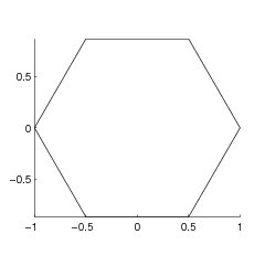
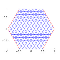
Fig. 1: Geometry (left) and a sample mesh $\mathcal{T}_{1/7}$ that consists of congruent and equilateral triangles of size $h=1/7$ (right) for Example 1.

For any positive integer $m$, let $\mathcal{T}_{1/m}$ denote the regular triangulation that consists of $6m^{2}$ congruent and equilateral triangles of size $h=1/m$. See Figure 1 (right) for a sample triangulation $\mathcal{T}_{1/7}$.

6.1 Stability

In this subsection, we use the following penalty parameters for the symmetric IPDG method (cf. (21)) according to Theorem 7 (or 12):

(71) $$\gamma_{1,e}=0.1,\quad\gamma_{0,e}=(k^{2}h)^{2/3}\gamma_{1}^{1/3},\quad\text{ and }\beta_{1,e}=1.$$

Given a triangulation $\mathcal{T}_{h}$, let $u_{h}^{\rm FEM}$ be the $P_{1}$-conforming finite element approximation of the problem (68)–(69). Recall that $u_{h}$ denotes the IPDG solution. Figure 2 plots the $H^{1}$-seminorm of the IPDG solution $\left\|u_{h}\right\|_{1,h}$, the $H^{1}$-seminorm of the finite element solution $\bigl{|}u_{h}^{\rm FEM}\bigr{|}_{H^{1}(\Omega)}$ for $h=0.05$ and $0.005$, respectively, and the $H^{1}$-seminorm of the exact solution $\bigl{|}u\bigr{|}_{H^{1}(\Omega)}$ for $k=1,\cdots,230.$ It is shown that

(72) $$\bigl{|}u\bigr{|}_{H^{1}(\Omega)}\simeq 1,\qquad\left\|u_{h}\right\|_{1,h}\lesssim 1,\qquad\bigl{|}u_{h}^{\rm FEM}\bigr{|}_{H^{1}(\Omega)}\lesssim 1.$$

We notice that the stability estimate $\left\|u_{h}\right\|_{1,h}\lesssim 1$ implies that $\left\|u_{h}\right\|_{L^{2}(\Omega)}\lesssim 1/k$. These stability estimates are better than those given by Theorem 7.

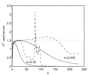
Fig. 2: $\left\|u_{h}\right\|_{1,h}$ (solid), $\bigl{|}u_{h}^{\rm FEM}\bigr{|}_{H^{1}(\Omega)}$ (dashed) for $h=0.05$ and $0.005$, respectively. The dotted line gives the $H^{1}$-seminorm of the exact solution $\bigl{|}u\bigr{|}_{H^{1}(\Omega)}$.

6.2 Error of the finite element interpolation

Given a triangulation $\mathcal{T}_{h}$, let $\hat{u}_{h}$ be the $P_{1}$-conforming finite element interpolation of $u$ on $\mathcal{T}_{h}$. Consider in Figure 3 log-log plots of the relative error $\hat{e}(h,k):=\bigl{|}u-\hat{u}_{h}\bigr{|}_{1}\big{/}\bigl{|}u\bigr{|}_{1}$ of the finite element interpolation in $H^{1}$-seminorm for different $k$ versus $1/h$. Similar to the 1-D case [37], All error curves decay with constant slope of $-1$. Note that the error stays at around 100% on coarse mesh and starts to decrease at a certain mesh size. We are interested in the mesh size where the descent starts. Similar to “the critical number of degrees of freedom” introduced in [37], we introduce the following definition of critical mesh size.

Definition 13.

Define—for any fixed $k$ and $f$—the critical mesh size as maximum mesh size $H(k,f)$ for which

1. $\tilde{e}(h,k)<1$ for $h<H(k,f)$, and

2. $\tilde{e}(h,k)\to 0$ as $h\to 0.$

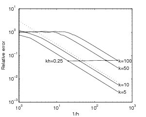
Fig. 3: Relative error of the finite element interpolation in $H^{1}$-seminorm for $k=5,k=10,k=50,$ and $k=100$. The dotted line gives the reference line with slope $-1$.

Recall that the critical mesh size for the one dimensional case is one half of the wavelength, that is, $\frac{\pi}{k}$ [37]. Since the solution $u$ is axial symmetric (cf. (70)) and the trace along any direction may be resolved by a mesh with mesh size less than $\frac{\pi}{k}$, the critical mesh size for the finite element interpolation should be greater than or equal to $\frac{\pi}{k}$. Figure 4 plots the reciprocal of the critical mesh size for the finite element interpolation computed for all integer $k$ from $1$ to $230$ and the line passing through the origin has slope $\frac{1}{\pi\sqrt{3}}$. It shows that

(73) $$\text{ the critical mesh size for }\hat{u}_{h}\approx\frac{\sqrt{3}\pi}{k}.$$

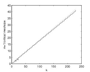
Fig. 4: Reciprocal of the critical mesh size of the relative error of the finite element interpolation in $H^{1}$-seminorm computed for $k=1,\cdots,230$. The dotted line gives the line through the origin with slope $\frac{1}{\pi\sqrt{3}}$.

Figure 3 also shows that the error of the finite element interpolation is controlled by the magnitude $kh$. For illustration, the points that are computed from $kh=0.25$ are connected. The connecting line does neither increase nor decrease significantly with the change of $k$. For more detailed observation, the relative errors of the finite element interpolations, computed for all integer $k$ from $1$ to $230$ for $kh=1$ and $kh=0.5$, are plotted in Figure 5. The error for $kh=1$ stays around $0.247$ and the error for $kh=0.25$ stays around $0.124$. Note that $0.124/0.247\approx 0.5$ which verifies that the relative error of the finite element interpolation in $H^{1}$-seminorm satisfies $\hat{e}(h,k)=O(kh).$

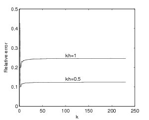
Fig. 5: Relative errors of the finite element interpolations in $H^{1}$-seminorm computed for $k=1,\cdots,230$ with mesh size $h$ determined by $kh=1$ and $kh=0.5$, respectively.

6.3 Error of the DG solution

From Theorem 11, the stability estimates in Subsection 6.1 suggest that the error of the IPDG solution in $H^{1}$-seminorm could be bounded by

(74) $$\bigl{|}u-u_{h}\bigr{|}_{1,h}\leq(1+kh)\big{(}C_{1}kh+C_{2}k^{3}h^{2}\big{)}$$

for some constants $C_{1}$ and $C_{2}$. The second term on the right hand side is the so-called pollution error. We now present numerical results which verify the above error bound.

In Figure 6, the relative error of the IPDG solution with parameters given by (71) and the relative error of the finite element interpolation are displayed in one plot. The relative error of the IPDG solution stays around $100\%$ before a critical mesh size is reached, then decays slowly on a range increasing with $k$, and then decays at a rate greater than $-1$ in the log-log scale but converges as fast as the finite element interpolation (with slope $-1$) for small $h$. The relative error grows with $k$ along line $kh=0.25.$ Unlike the error of the finite element interpolation, the error of the IPDG solution is not controlled by the magnitude of $kh$ — see also Figure 7.

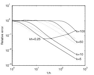
Fig. 6: Relative error of the IPDG solution with parameters given by (71) (solid) and relative error of the finite element interpolation (dotted) in $H^{1}$-seminorm for $k=5,k=10,k=50,$ and $k=100$, respectively.

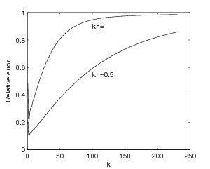
Fig. 7: Relative errors of the IPDG solutions with parameters given by (71) in $H^{1}$-seminorm computed for $k=1,\cdots,230$ with mesh size $h$ determined by $kh=1$ and $kh=0.5$, respectively.

Figure 8 plots the relative error of the IPDG solution with parameters given by (71) for $k=5^{2/3},10^{2/3},\cdots,500^{2/3}$ and $h$ determined by $k^{3}h^{2}=1$. The error does not increase with respect to $k$ which verifies (74).

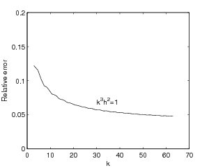
Fig. 8: Relative errors of the IPDG solutions with parameters given by (71) in $H^{1}$-seminorm computed for $k=5^{2/3},10^{2/3},\cdots,500^{2/3}$ with mesh size $h$ determined by $k^{3}h^{2}=1$.

Figure 9 plots the reciprocal of the critical mesh size for the IPDG solution with parameters given by (71) computed for all integer $k$ from $1$ to $230$ and the lines passing through the origin have slopes $\frac{1}{1.35\pi}$ and $\frac{1}{\pi}$, respectively. It shows that

(75) $$\text{ the critical mesh size for }u_{h}\approx\frac{1.35\pi}{k}$$

with two exceptions but they are still less than $\frac{\pi}{k}.$ It is interesting that the dependence on $1/k$ is essentially linear. We consider the IPDG solution with parameters given by (71) for $k=100$ on the mesh with mesh size $h=1/60$. The relative error in $H^{1}$-seminorm is about 0.9898. Figure 10 presents the surface plots of the interpolation (left) and the IPDG solution (right). It is shown that the IPDG solution has a correct shape although its amplitude is not very accurate.

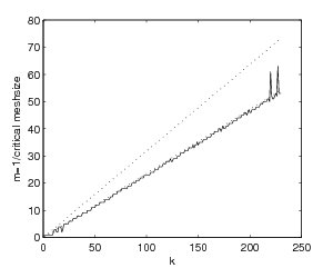
Fig. 9: Reciprocal of the critical mesh size of the relative error of the IPDG solution with parameters given by (71) in $H^{1}$-seminorm computed for $k=1,\cdots,230$. The dotted lines give the lines through the origin with slopes $\frac{1}{1.35\pi}$ and $\frac{1}{\pi}$.

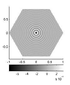
Fig. 10: Surface plots of the interpolation (left) and the IPDG solution (right) with parameters given by (71) for $k=100$ on the mesh with mesh size $h=1/60$.

6.4 Sensitivity of the error bounds with respect to penalty parameters

In this subsection, we examine the sensitivity of the error of the IPDG solution in $H^{1}$-seminorm with respect to the parameters $\gamma_{0,e}$, $\beta_{1,e}$, and $\gamma_{1,e}$, respectively.

First, we examine the sensitivity of the error in $\gamma_{0,e}$. To the end, for $k=5$ and $k=50$, respectively, we fix $\gamma_{1,e}=0.1$ and $\beta_{1,e}=1$, and compute the IPDG solution with the following $\gamma_{0,e}$: $\gamma_{0,e}=(k^{2}h)^{2/3}\gamma_{1,e}^{1/3}$ (see (71)), $\gamma_{0,e}=1$, $\gamma_{0,e}=0.01$, and $\gamma_{0,e}=100$. Figure 11 plots the relative error of the IPDG solution for each run. We observe that the error in the $H^{1}$-seminorm is not sensitive with respect to the parameter $\gamma_{0,e}$. It is clear that $\gamma_{0,e}$ affects the continuity of the solution. The larger the parameter $\gamma_{0,e}$, the more continuous the IPDG solution.

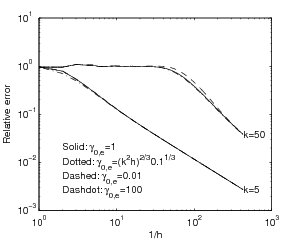
Fig. 11: Relative error of the IPDG solution with parameters $\gamma_{1,e}=0.1,\beta_{1,e}=1$, and each of following $\gamma_{0,e}$: $\gamma_{0,e}=(k^{2}h)^{2/3}\gamma_{1,e}^{1/3}$ (dotted), $\gamma_{0,e}=1$ (solid), $\gamma_{0,e}=0.01$ (dashed), and $\gamma_{0,e}=100$ (dashdot) in the $H^{1}$-seminorm for $k=5$ and $k=50$, respectively.

Secondly, we test the sensitivity of the error in $\beta_{1,e}$. Figure 12 plots the relative error in the $H^{1}$-seminorm of the IPDG solution with parameters $\gamma_{0,e}=1,\gamma_{1,e}=0.1$, and each of the following $\beta_{1,e}$: $\beta_{1,e}=0,1,100$, for $k=5$ and $k=50$, respectively. Again, we observe that the error in the $H^{1}$-seminorm is not sensitive with respect to the parameter $\beta_{1,e}$.

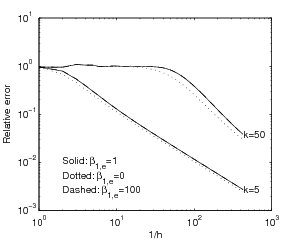
Fig. 12: Relative error in the $H^{1}$-seminorm of the IPDG solution with parameters $\gamma_{0,e}=1,\gamma_{1,e}=0.1$, and each of the following $\beta_{1,e}$: $\beta_{1,e}=0$ (dotted), $\beta_{1,e}=1$ (solid), and $\beta_{1,e}=100$ (dashed) for $k=5$ and $k=50$, respectively.

Finally, we examine the sensitivity of the error in $\gamma_{1,e}$. To the end, we fix $\gamma_{0,e}=1$ and $\beta_{1,e}=1$ and compute the IPDG solution with the following $\gamma_{1,e}$: $\gamma_{1,e}=0,0.01,0.1,1$ for $k=5$ and $k=50$, respectively. Figure 13 plots the relative error in the $H^{1}$-seminorm of the IPDG solution for each run. We observe that the error has a similar behavior as the error of the finite element solution for small value $\gamma_{1,e}=0,0.01$ (cf. Figure 16) and the solution is more stable for larger $\gamma_{1,e}$, but a large $\gamma_{1,e}$, say $\gamma_{1,e}=1$, may result in a large (absolute) error.

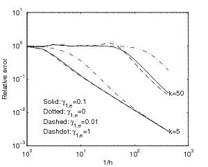
Fig. 13: Relative error in the $H^{1}$-seminorm of the IPDG solution with parameters $\gamma_{0,e}=1,\beta_{1,e}=1$, and each of the following $\gamma_{1,e}$: $\gamma_{1,e}=0.1$ (solid), $\gamma_{1,e}=0$ (dotted), $\gamma_{1,e}=0.01$ (dashed), and $\gamma_{1,e}=1$ (dashdot) for $k=5$ and $k=50$, respectively.

6.5 Reduction of the pollution effect

One advantage of the IPDG method is that it contains several parameters which can be tuned for a particular purpose. In [2], it is shown that it is possible to reduce the pollution error of the IPDG method by choosing appropriate parameters $\sigma$ and ${\rm\mathbf{i}}\gamma_{0,e}$. Recall that all choice of $\sigma$ but one lead to non-symmetric formulations. In this subsection, we shall show that appropriate choice of the parameter $\gamma_{1,e}$ can significantly reduce the pollution error of the symmetric IPDG method (with $\sigma=1$). We use the following parameters:

(76) $${\rm\mathbf{i}}\gamma_{1,e}=-0.07+0.01{\rm\mathbf{i}},\quad\gamma_{0,e}=100,\quad\text{ and }\beta_{1,e}=1.$$

We remark that ${\rm\mathbf{i}}\gamma_{1,e}$ is simply chosen from the set $\left\{0.01(p+q{\rm\mathbf{i}}),-50\leq p,q\leq 50\right\}$ to minimize the relative error of the IPDG solution in $H^{1}$-seminorm with $\gamma_{0,e}=100$ and $\beta_{1,e}=1$ for wave number $k=50$ and mesh size $h=1/20.$

In Figure 14, the relative error of the IPDG solution with parameters given by (76) and the relative error of the finite element interpolation are displayed in one plot. The IPDG method with parameters given by (76) is much better than the IPDG method using parameters given by (71) (cf. Figure 6). The relative error does neither increase nor decrease significantly with the change of $k$ along line $kh=0.25$ for $k\leq 100$. But this does not mean that the pollution error has been eliminated.

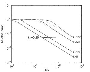
Fig. 14: Relative error of the IPDG solution with parameters given by (76) (solid) and relative error of the finite element interpolation (dotted) in $H^{1}$-seminorm for $k=5,k=10,k=50,$ and $k=100$, respectively.

For more detailed observation, the relative errors of the IPDG solution with parameters given by (76), computed for all integer $k$ from $1$ to $230$ for $kh=1$ and $kh=0.5$, are plotted in Figure 15. It is shown that the pollution error is reduced significantly (cf. Figure 7 and Figure 5).

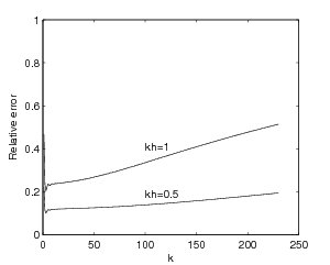
Fig. 15: Relative errors of the IPDG solution with parameters given by (76) in $H^{1}$-seminorm computed for $k=1,\cdots,230$ with mesh size $h$ determined by $kh=1$ and $kh=0.5$, respectively.

6.6 Comparison between the IPDG solution and the finite element solution

We have shown the flexibility and performance of the IPDG method in previous subsections. In this subsection, we give a comparison between the IPDG method and the finite element method. One disadvantage of the IPDG method compared to the finite element method is that the linear system of the IPDG discretization involves more number of degrees of freedom than that of finite element discretization on the same mesh. In two dimensional case it is about three times more. So in the asymptotic range, the IPDG method is less effective in terms of number of degrees of freedom. We shall show that, for Problem (68)–(69), the IPDG solution is more stable than the finite solution for large $h$, and it is possible to choose appropriate parameters such that the IPDG method is more effective than the finite element method in preasymptotic range even in terms of number of degrees of freedom.

In Figure 16, the relative error of the finite element solution and the relative error of the finite element interpolation are displayed in one plot. The relative error of the finite element solution first oscillates around $100\%$, then decays at a rate greater than $-1$ in the log-log scale but converges as fast as the finite element interpolation (with slope $-1$) for small $h$. The relative error grows with $k$ along line $kh=0.25.$ The error of the finite element solution is not controlled by the magnitude of $kh$ — see also Figure 17.

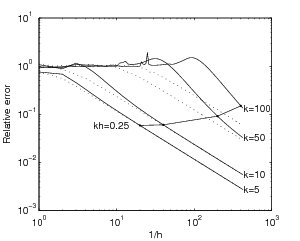
Fig. 16: Relative error of the finite element solution (solid) and relative error of the finite element interpolation (dotted) in $H^{1}$-seminorm for $k=5,k=10,k=50,$ and $k=100$, respectively.

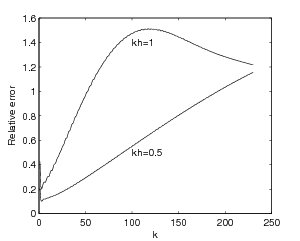
Fig. 17: Relative errors of the finite element solutions in $H^{1}$-seminorm computed for $k=1,\cdots,230$ with mesh size $h$ determined by $kh=1$ and $kh=0.5$, respectively.

Figure 18 plots the reciprocal of the critical mesh size for the finite element solution computed for all $k$ from $1$ to $230$ and the curve $m=\sqrt{k^{3}/48}$. It is shown that

(77) $$\text{ the critical mesh size for }u_{h}^{\rm FEM}\approx\sqrt{\frac{48}{k^{3}}}.$$

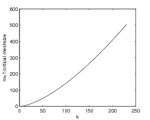
Fig. 18: Reciprocal of the critical mesh size of the relative error of the finite element solution in $H^{1}$-seminorm computed for $k=1,\cdots,230$. The dotted line gives the curve $m=\sqrt{k^{3}/48}$.

We can see that the IPDG solution is more stable than the finite element solution. For more detailed comparison, we consider the problem (68)–(69) with wave number $k=100$. The traces of the IPDG solutions with parameters given by (76) and the finite element solutions in the $xz$-plane for mesh sizes $h=1/50,1/120$, and $1/200$, and the trace of the exact solution in the $xz$-plane, are plotted in Figure 19. The shape of the IPDG solution is roughly same as that of the exact solution for $h=1/50,$. They matches very well for $h=1/120$ and even better for $h=1/200$. While the finite element solution has a wrong shape near the origin for $h=1/50$ and $h=1/120$ and only has a correct shape for $h=1/200$. The phase error appears in all the three cases for the finite element solution.

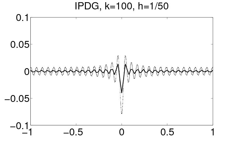
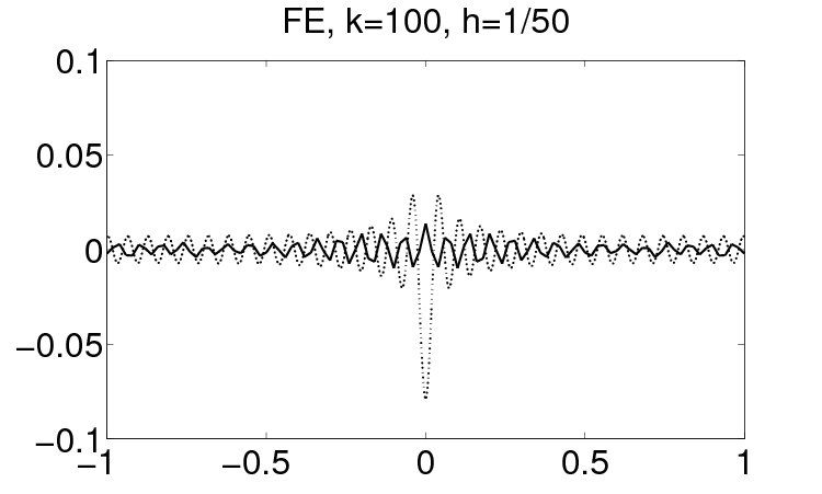
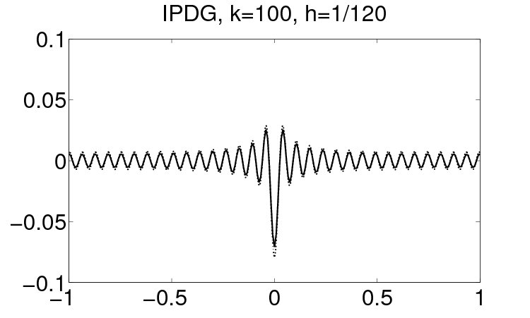
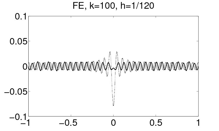
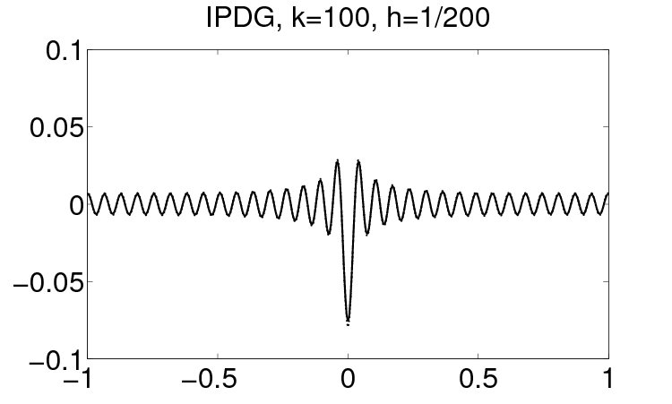
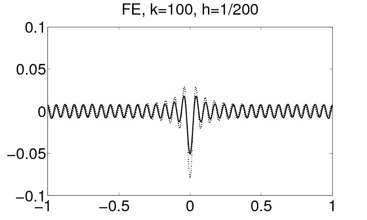
Fig. 19: The traces of the IPDG solutions (left) with parameters given by (76) and the finite element solutions (right) in the $xz$-plane for $k=100$ and mesh sizes $h=1/50,1/120$, and $1/200$, respectively. The dotted lines give the trace of the exact solution in the $xz$-plane.

Table 1 shows the numbers of degrees of freedom needed for $30$% relative errors in $H^{1}$-seminorm for the finite element interpolation, the IPDG solution with parameters given by (76), and the finite element solution, respectively. The finite element method needs less DOFs when $k=10$ and $k=50$ than the IPDG method does, but the situation reverses when $k=100$ and $k=200$.

k	10	50	100	200
Interpolation	217 (1/8)	5,167 (1/41)	20,419 (1/82)	81,181 (1/164)
IPDG	1,152 (1/8)	38,088 (1/46)	217,800 (1/110)	1,431,432 (1/282)
FEM	397 (1/11)	30,301 (1/100)	229,357 (1/276)	1,804,201 (1/775)

Table 1: Numbers of degrees of freedom needed for 30% relative errors in $H^{1}$-seminorm for the finite element interpolation, the IPDG solution with parameters given by (76), and the finite element solution, respectively. The fractions in the parentheses give the corresponding mesh sizes.

References

- [1] M. Ainsworth, P. Monk, and W. Muniz. Dispersive and dissipative properties of discontinuous Galerkin finite element methods for the second-order wave equation. J. Sci. Comput., 27:5–40, 2006.
- [2] G. B. Alvarez, A. F. D. Loula, E. G. Dutra do Carmo, F. A. Rochinha. A discontinuous finite element formulation for Helmholtz equation. Comput. Methods Appl. Mech. Engrg., 195:4018–4035, 2006.
- [3] D. Arnold. An interior penalty finite element method with discontinuous elements. SIAM J. Numer. Anal., 19:742–760, 1982.
- [4] D. Arnold, F. Brezzi, B. Cockburn, and D. Marini. Unified analysis of discontinuous Galerkin methods for elliptic problems. SIAM J. Numer. Anal., 39:1749–1779, 2001.
- [5] A. K. Aziz and R. B. Kellogg. A scattering problem for the Helmholtz equation. In Advances in computer methods for partial differential equations, III (Proc. Third IMACS Internat. Sympos., Lehigh Univ., Bethlehem, Pa., 1979), pages 93–95. IMACS, New Brunswick, N.J., 1979.
- [6] A. K. Aziz and A. Werschulz. On the numerical solutions of Helmholtz’s equation by the finite element method. SIAM J. Numer. Anal., 17(5):681–686, 1980.
- [7] I. Babuška, U. Banerjee, and J. Osborn. Survey of meshless and generalized finite element methods: a unified approach. Acta Numer., pp. 1-125, 2003.
- [8] I. Babuška, U. Banerjee, and J. Osborn. Generalized finite element method - main ideas, results, and perspective. Inter. J. of Comput. Methods, 1(1):67–103, 2004.
- [9] I. Babuška, F. Ihlenburg, E. T. Paik, and S. A. Sauter. A generalized finite element method for solving the Helmholtz equation in two dimensions with minimal pollution. Comput. Methods Appl. Mech. Engrg., 128(3-4):325–359, 1995.
- [10] I. M. Babuška and S. A. Sauter. Is the pollution effect of the FEM avoidable for the Helmholtz equation considering high wave numbers? SIAM J. Numer. Anal., 34(6):2392–2423, 1997.
- [11] G. A. Baker. Finite element methods for elliptic equations using nonconforming elements. Math. Comp., 31:44–59, 1977.
- [12] G. Bao. Finite element approximation of time harmonic waves in periodic structures. SIAM J. Numer. Anal., 32(4):1155–1169, 1995.
- [13] J.-P. Berenger. A perfectly matched layer for the absorption of electromagnetic waves. J. Comput. Phys., 114(2):185–200, 1994.
- [14] S. Brenner and R. Scott. The Mathematical Theory of Finite Element Methods. Springer-Verlag, New York, 1994.
- [15] C. L. Chang. A least-squares finite element method for the Helmholtz equation. Comput. Methods Appl. Mech. Engrg., 83(1):1–7, 1990.
- [16] Z. Chen and H. Wu. An adaptive finite element method with perfectly matched absorbing layers for the wave scattering by periodic structures. SIAM J. Numer. Anal., 41:799–826, 2003.
- [17] E. T. Chung, and B. Engquist. Optimal discontinuous Galerkin methods for wave propagation. SIAM J. Numer. Anal., 44(5):2131–2158, 2006.
- [18] P. G. Ciarlet. The Finite Element Method for Elliptic Problems. North-Holland, Amsterdam, 1978.
- [19] B. Cockburn, G. E. Karniadakis, C.-W. Shu. Discontinuous Galerkin Methods, Theory, Computation, and Applications, Springer lecture Notes in Computational Science and Engineering, vol. 11. Springer-Verlag, 2000.
- [20] B. Cockburn and C. -W. Shu. The local discontinuous Galerkin method for convection-diffusion systems. SIAM J. Numer. Anal., 35:2440–2463, 1998.
- [21] D. Colton and P. Monk. The numerical solution of the three-dimensional inverse scattering problem for time harmonic acoustic waves. SIAM J. Sci. Statist. Comput., 8(3):278–291, 1987.
- [22] D. Colton and R. Kress. Inverse acoustic and electromagnetic scattering theory. Springer-Verlag, Berlin, 1992.
- [23] P. Cummings. Analysis of Finite Element Based Numerical Methods for Acoustic Waves, Elastic Waves and Fluid-Solid Interactions in the Frequency Domain. PhD thesis, The University Tennessee, 2001.
- [24] P. Cummings and X. Feng. Sharp regularity coefficient estimates for complex-valued acoustic and elastic Helmholtz equations. M3AS, 16:139–160, 2006.
- [25] J. Douglas, Jr. and T. Dupont. Interior penalty procedures for elliptic and parabolic Galerkin methods. Lecture Notes In Physics 58, Springer Verlag, Berlin, 1976.
- [26] J. Douglas, Jr., J. E. Santos, D. Sheen, and L. S. Bennethum. Frequency domain treatment of one-dimensional scalar waves. Math. Models Methods Appl. Sci., 3(2):171–194, 1993.
- [27] J. Douglas, Jr., D. Sheen, and J. E. Santos. Approximation of scalar waves in the space-frequency domain. Math. Models Methods Appl. Sci., 4(4):509–531, 1994.
- [28] B. Engquist and A. Majda. Radiation boundary conditions for acoustic and elastic wave calculations. Comm. Pure Appl. Math., 32(3):314–358, 1979.
- [29] B. Engquist, and O. Runborg. Computational high frequency wave propagation. Acta Numer., 12:181–266, 2003.
- [30] X. Feng. Absorbing boundary conditions for electromagnetic wave propagation. Math. Comp., 68(225):145–168, 1999.
- [31] X. Feng and O. A. Karakashian. Fully discrete dynamic mesh discontinuous Galerkin methods for the Cahn-Hilliard equation of phase transition. Math. Comp., 76:1093–1117, 2007.
- [32] X. Feng and H. Wu. -discontinuous Galerkin methods for the Helmholtz equation with large wave numbers, in preparation.
- [33] C. I. Goldstein. The finite element method with nonuniform mesh sizes applied to the exterior Helmholtz problem. Numer. Math., 38(1):61–82, 1981.
- [34] I. Harari and T. J. R. Hughes. Analysis of continuous formulations underlying the computation of time-harmonic acoustics in exterior domains. Comput. Methods Appl. Mech. Engrg., 97(1):103–124, 1992.
- [35] U. Hetmaniuk. Stability estimates for a class of Helmholtz problems. Commun. Math. Sci., 5(3):665–678, 2007.
- [36] F. Ihlenburg. Finite Element Analysis of Acoustic Scattering. Springer-Verlag, New York, 1998.
- [37] F. Ihlenburg and I. Babuška. Finite element solution of the Helmholtz equation with high wave number. I. The -version of the FEM. Comput. Math. Appl., 30(9):9–37, 1995.
- [38] I. Perugia. A note on the discontinuous Galerkin approximation of the Helmholtz equation. preprint
- [39] N. A. Kampanis, J. Ekaterinaris, and V. Dougalis. Effective Computational Methods for Wave Propagation, Chapman & Hall/CRC, 2008.
- [40] J. M. Melenk. On Generalized Finite Element Methods. PhD thesis, University of Maryland at College Park, 1995.
- [41] J. M. Melenk and I. Babuška. The partition of unity finite element method: basic theory and applications. Comput. Methods Appl. Mech. Engrg., 139(1-4):289–314, 1996.
- [42] A. A. Oberai and P. M. Pinsky. A multiscale finite element method for the Helmholtz equation. Comput. Methods Appl. Mech. Engrg., 154(3-4):281–297, 1998.
- [43] B. Rivière, M. F. Wheeler, and V. Girault. Improved energy estimates for interior penalty, constrained and discontinuous Galerkin methods for elliptic problems. I. Comput. Geosci., 3(3-4):337–360 (2000), 1999.
- [44] A. H. Schatz. An observation concerning Ritz–Galerkin methods with indefinite bilinear forms. Math. Comp., 28:959–962, 1974.
- [45] J. Shen and L. Wang. Analysis of a spectral-Galerkin approximation to the Helmholtz equation in exterior domains. SIAM J. Numer. Anal., 45:1954–1978, 2007.
- [46] J.T. Oden and C.E. Baumann. A conservative DGM for convection-diffusion and Navier-Stokes problems. Proceedings of the International Symposium on the discontinuous Galerkin method (B. Cockburn, G. E. Karniadakis, C.-W. Shu Eds.), Springer lecture notes in Computational Science and Engineering, vol. 11, 2000, pp.179–196.
- [47] M. F. Wheeler. An elliptic collocation-finite element method with interior penalties. SIAM J. Numer. Anal., 15:152–161, 1978.
- [48] D.-h. Yu. Natural Boundary Integral Method and its Applications. Mathematics and its Applications, Vol. 539, Kluwer Academic Publishers, Dordrecht, 2002.
- [49] O. C. Zienkiewicz. Achievements and some unsolved problems of the finite element method. Internat. J. Numer. Methods Engrg, 47:9–28, 2000.