Stochastic quantization at nonzero chemical potential

Abstract:

Lattice QCD at finite chemical potential is difficult due to the sign problem. We use stochastic quantization and complex Langevin dynamics to study this issue. First results for QCD in the hopping expansion are encouraging. U(1) and SU(3) one link models are used to gain further insight into why the method appears to be successful.

1 Introduction

QCD at finite chemical potential is difficult because the complex fermion determinant prohibits lattice techniques based on direct importance sampling, while reweighting methods suffer from sign and overlap problems. Stochastic quantization [1] is an alternative nonperturbative method which in principle can deal with complex actions, via the use of complex Langevin dynamics [2, 3, 4, 5]. However, since proposed in the 80’s, progress has been hindered by numerical instabilities and uncertainty about or lack of convergence (see e.g. Refs. [6, 7] for relevant work). Recently it was shown in the context of nonequilibrium (Minkowski) quantum field dynamics that some of these problems could be alleviated by the use of more refined Langevin algorithms [8, 9, 10]. These studies motivated us to consider euclidean systems at finite chemical potential, either derived from or with a structure similar to QCD at finite density. The first results are very promising and can be found in Ref. [11].

2 Three models with a sign problem and complex Langevin dynamics

We consider three models inspired by or derived from QCD. The partition functions have the familiar form

$$Z=\int DU\,e^{-S_{B}}\det M,\;\;\;\;\;\;\;\;\;\mbox{with}\;\;\;\;\;\;\;\;\;\det M(\mu)=[\det M(-\mu)]^{*}.$$ (1)

Here $S_{B}$ is the real bosonic action, depending on the gauge links $U$, and $\det M$ is the complex fermion determinant, with $\mu$ the chemical potential.

QCD in the hopping expansion: The (Wilson) fermion matrix reads

$$M=1-\kappa\sum_{i=1}^{3}\mbox{space}-\kappa\left(e^{\mu}\Gamma_{+4}U_{x,4}T_{4}+e^{-\mu}\Gamma_{-4}U_{x,4}^{-1}T_{-4}\right).$$ (2)

In the hopping expansion at nonzero $\mu$, $\kappa$ is taken to $0$ but terms with $\kappa e^{\pm\mu}$ are preserved. As a result, only the temporal links survive and the determinant is local,

$$\det M \approx \det\left[1-\kappa\left(e^{\mu}\Gamma_{+4}U_{x,4}T_{4}+e^{-\mu}\Gamma_{-4}U_{x,4}^{-1}T_{-4}\right)\right]$$ (3)

$$= \prod_{{\mathbf{x}}}\det\left(1+he^{\mu/T}{\cal P}_{{\mathbf{x}}}\right)^{2}\det\left(1+he^{-\mu/T}{\cal P}_{{\mathbf{x}}}^{-1}\right)^{2}.$$

Here $h=(2\kappa)^{N_{\tau}}$ and ${\cal P}_{\mathbf{x}}^{(-1)}$ are the (conjugate) Polyakov loops. The gauge action is the standard Wilson action, $S_{B}=-\beta\sum_{P}(\frac{1}{6}[\mbox{Tr}\,U_{P}+\mbox{Tr}\,U_{P}^{-1}]-1)$ and is preserved completely.

In order to investigate the algorithm in detail, we have also studied two one link models, where exact results are available.

SU(3) one link model: The bosonic action is $S_{B}=-\frac{\beta}{6}(\mbox{Tr}\,U+\mbox{Tr}\,U^{-1})$, with $U\in$ SU(3). The determinant has the product form as above,

$$\det M=\det\left(1+\kappa e^{\mu}U\right)\left(1+\kappa e^{-\mu}U^{-1}\right).$$ (4)

Exact results follow from integration over the reduced Haar measure.

U(1) one link model: The bosonic action is $S_{B}=-\frac{\beta}{2}(U+U^{-1})$ and the determinant is $\det M=1+\frac{\kappa}{2}\left(e^{\mu}U+e^{-\mu}U^{-1}\right)$. When the link is written as $U=e^{ix}$, the partition function is a one-dimensional integral,

$$Z=\int_{-\pi}^{\pi}\frac{dx}{2\pi}\,e^{\beta\cos x}\left[1+\kappa\cos(x-i\mu)\right],$$ (5)

and exact expressions are available in terms of Bessel functions.

All models behave in the same way as QCD under the substitution $\mu\to-\mu$. Observables investigated are the (conjugate) Polyakov loops, the density and the phase of the determinant.

Since the determinants are complex, standard lattice methods cannot be used. We employ complex Langevin dynamics instead. The Langevin update [for SU(3)] is

$$U(\theta+\epsilon)=R(\theta)\,U(\theta),\;\;\;\;\;\;\;\;\;\;\;\;\;\;\;\;R=\exp\left[i\lambda_{a}\left(\epsilon K_{a}+\sqrt{\epsilon}\eta_{a}\right)\right],$$ (6)

where $\theta$ is the Langevin time, $\epsilon$ is the stepsize, $\lambda_{a}$ ($a=1,\ldots,8$) are the Gell-Mann matrices, the drift term reads

$$K_{a}=-D_{a}S_{\rm eff},\;\;\;\;\;\;\;\;\;\;\;\;S_{\rm eff}=S_{B}+S_{F},\;\;\;\;\;\;\;\;\;\;\;\;S_{F}=-\ln\det M,$$ (7)

with $D_{a}f(U)=\partial_{\alpha}f(e^{i\alpha\lambda_{a}}U)|_{\alpha=0}$, and the noise satisfies

$$\langle\eta_{a}\rangle=0,\;\;\;\;\;\;\;\;\;\;\;\;\;\;\;\;\langle\eta_{a}\eta_{b}\rangle=2\delta_{ab},$$ (8)

suppressing euclidean spacetime indices. Since the action and as a result the drift term are complex, $R^{\dagger}R\neq 1\!\!\!1$, although $\det R=1$ still holds. Therefore the complex Langevin dynamics takes place in SL(3, $\mathbb{C}$) and not in SU(3). We come back to this below. Related to this, we note that after complexification observables should be defined in terms of $U$ and $U^{-1}$, but not of $U^{\dagger}\neq U^{-1}$.

3 Results

The complex Langevin equation (6) was solved numerically, with a stepsize $\epsilon=2-5\times 10^{-5}$. In the one link models, we have not observed any instability or runaway solution. In the field theory, runaways have been eliminated by being careful with numerical precision and roundoff errors, and employing a dynamical stepsize. Here we show some results for illustration; a more extensive discussion can be found in Ref. [11].

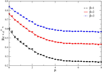
Figure 1: Real part of the Polyakov loop $\langle e^{ix}\rangle$ as a function of $\mu$ (left) and the plaquette $\langle\cos x\rangle$as a function of $\mu^{2}$ (right) for three values of $\beta$ at fixed $\kappa=1/2$ in the U(1) one link model. The lines are the analytical results, the symbols are obtained with Langevin dynamics.

The Polyakov loop $\mbox{Re}\,\langle e^{ix}\rangle$ in the U(1) model is shown in Fig. 1 (left). The data points come from the Langevin dynamics, the lines are the exact solutions. Excellent agreement is observed. At imaginary chemical potential, $\mu=i\mu_{I}$, the determinant is real and there is no need to complexify the Langevin dynamics. The smooth connection between the results obtained with complex Langevin (when $\mu^{2}>0$) and real Langevin (when $\mu^{2}<0$) is shown in Fig. 1 (right) for the plaquette $\langle\cos x\rangle$. In particular, statistical errors are comparable. We note here that also in the SU(3) one link model, excellent agreement between exact and numerical results can be seen [11].

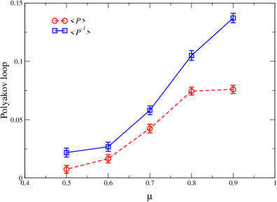
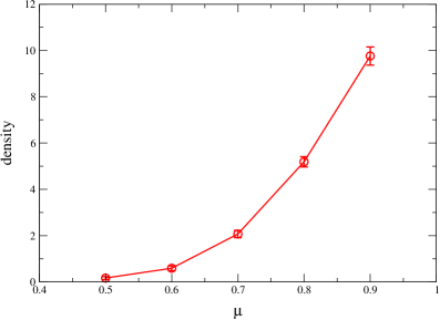
Figure 2: Real part of the Polyakov loop $\langle P\rangle$ and the conjugate Polyakov loop $\langle P^{-1}\rangle$ (left) and the density $\langle n\rangle$ (right) as a function of $\mu$ at $\beta=5.6$, $\kappa=0.12$ on a $4^{4}$ lattice, with $N_{f}=3$ flavours.

First results for the QCD in the hopping expansion are shown in Fig. 2 for the (conjugate) Polyakov loops $P^{(-1)}=\frac{1}{3}\mbox{Tr}\,{\cal P}^{(-1)}$ (left) and the density $\langle n\rangle=T\partial\ln Z/\partial\mu$, with $T=1/N_{\tau}$ (right). These results are obtained on a $4^{4}$ lattice at $\beta=5.6$. We observe that the (conjugate) Polyakov loops increase from a small value at $\mu=0.5$ to a value clearly different from zero at the larger $\mu$ values. Similarly, the density increases substantially with chemical potential. We interpret this as indications for a transition from a low-density “confining” phase to a high-density “deconfining” phase.

The sign problem in these models can be studied by writing the determinant as $\det M(\mu)=[\det M(-\mu)]^{*}=|\det M(\mu)|e^{i\phi}$ and considering the average phase factor

$$\langle e^{2i\phi}\rangle=\left\langle\frac{\det M(\mu)}{\det M(-\mu)}\right\rangle.$$ (9)

Scatter plots of $e^{2i\phi}$ during the Langevin evolution in QCD in the hopping expansion are shown in Fig. 3 (left). At zero chemical potential $\mbox{Re}\,e^{2i\phi}=1$, $\mbox{Im}\,e^{2i\phi}=0$. At nonzero $\mu$, we observe that phase fluctuations suddenly increase enormously. This behaviour is not unexpected when the sign problem is severe. For instance, the variance of the phase, $\langle\phi^{2}\rangle-\langle\phi\rangle^{2}$, is large and proportional to the four volume $N_{\sigma}^{3}N_{\tau}$. We emphasize, however, that the observables (Polyalov loop, density) are under control, with a reasonable numerical error. This suggests that phase fluctuations and the sign problem may not be a problem for this approach.

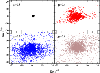
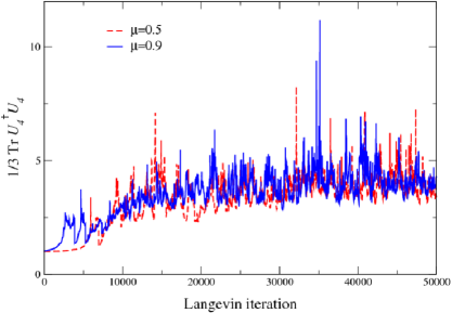
Figure 3: Left: Scatter plot of $e^{2i\phi}=\det M(\mu)/\det M(-\mu)$ during the Langevin evolution for various values of $\mu$ at $\beta=5.6$, $\kappa=0.12$ on a $4^{4}$ lattice. Right: Deviation from SU(3), $\mbox{Tr}\,U_{4}^{\dagger}U_{4}/3$ during the Langevin evolution, for $\mu=0.5$ and $0.9$.

Because of the complexification, the dynamics no longer takes place in SU(3) but in SL(3, $\mathbb{C}$) instead. When the links are written in terms of gauge potentials, $U=e^{i\lambda_{a}A_{a}/2}$, this implies that the $A_{a}$’s are now complex. A measure of how much the dynamics deviates from SU(3) can be given by considering $\frac{1}{N}\mbox{Tr}\,U^{\dagger}U$ which $=1$ if $U\in$ SU($N$) and $\geq 1$ if $U\in$ SL($N$, $\mathbb{C}$). Note that this observable is not analytic in $U$; it therefore does not correspond to an observable in the original gauge theory before complexification. In Fig. 3 (right) we show the Langevin time dependence of $\frac{1}{3}\mbox{Tr}\,U_{4}^{\dagger}U_{4}$ on the $4^{4}$ lattice for $\mu=0.5$ and $0.9$. After the thermalization stage, we observe a distinct deviation from 1, as expected. What is important is that the observable remains bounded during the evolution and does not run away to infinity.

Some insight into why stochastic quantization works at finite chemical potential can be obtained from the simple U(1) one link model. Consider the link $U=e^{ix}$ after complexification, with $x\to x+iy$. The Langevin equations are $\dot{x}=K_{x}+\eta$, $\dot{y}=K_{y}$, where $K_{x,y}$ are classical forces and the dot indicates a $\theta$ derivative. Classical flow diagrams in the $x$–$y$ plane are shown in Fig. 4. We find a stable fixed point at $x=0$ and unstable fixed points at $x=\pi$. The important observation is that this structure is independent of $\mu$. The small (blue) dots indicate a trajectory during the Langevin evolution. As is clearly visible, in the vertical (unbounded) direction the dynamics is attracted to the stable fixed point and remains bounded.

These flow diagrams are also useful to illustrate how the method is distinct from other approaches based on employing configurations obtained at zero chemical potential (reweighting, Taylor expansion). In the language of this simple model, in those approaches configurations are generated without an imaginary component of the gauge potential (i.e. $y=0$), and these are subsequently used to probe the system at finite chemical potential. In contrast, in this approach configurations have nonzero imaginary parts of the gauge potential ($y\neq 0$) and change therefore in an essential way when $\mu$ departs from zero, as indicated by comparing the two plots in Fig. 4.

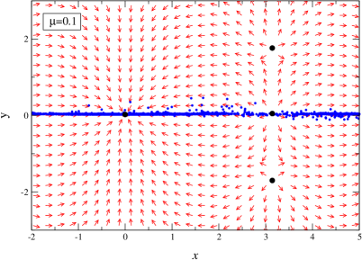
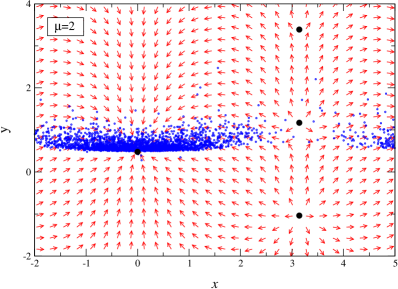
Figure 4: Classical flow diagram in the U(1) one link model. The horizontal $x$ (vertical $y$) axis corresponds to the real (imaginary) part of the gauge potential. The big dots indicate the fixed points at $x=0$ and $\pi$. The small circles indicate a trajectory during the Langevin evolution. Note the periodicity $x\to x+2\pi$. Parameters are $\beta=1$, $\kappa=1/2$, $\mu=0.1$ (left) and $\mu=2$ (right).

A second indication for the success of this approach in the U(1) model comes from an analysis of the complex Fokker-Planck equation for the $\theta$ dependent distribution $P(x,\theta)$,

$$\frac{\partial P(x,\theta)}{\partial\theta}=\frac{\partial}{\partial x}\left(\frac{\partial}{\partial x}+\frac{\partial S}{\partial x}\right)P(x,\theta).$$ (10)

We have solved this equation for the modes $P_{n}(\theta)=\int_{-\pi}^{\pi}e^{inx}P(x,\theta)/2\pi$ and a typical result is shown in Fig. 5 (left). A rapid convergence to the correct distribution $P(x)\sim e^{-S(x)}$ is observed. This behaviour can be understood from the eigenvalues of the complex Fokker-Planck operator. It follows from the symmetries of the model under $\mu\to-\mu$, $x\to-x$ that the eigenvalues are real. We found numerically that the nonzero eigenvalues are positive definite, see Fig. 5 (right). Although these results are not sufficient to prove convergence of the complexified dynamics analytically, it supports the stochastic results presented above.

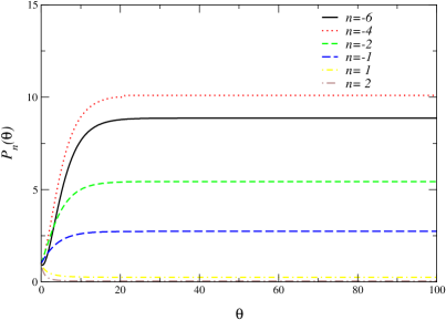
Figure 5: Left: Langevin evolution of the modes $P_{n}(\theta)$ of the complex Fokker-Planck distribution in the U(1) one link model ($\beta=1$, $\kappa=1/2$, $\mu=3$). Right: Smallest nonzero eigenvalues of the complex Fokker-Planck operator as a function of $\beta$ for various values of $\mu$ at $\kappa=1/2$.

4 Conclusion

We have considered complex Langevin dynamics to study theories with a complex action due to a chemical potential. In the U(1) and SU(3) one link models the agreement between exact and stochastic results is excellent. Moreover, in these simple models it is possible to gain insight into why the method works, using classical flow diagrams and an analysis of the eigenvalues of the complex Fokker-Planck operator. First results in QCD in the hopping expansion are very encouraging. Even though the phase of the determinant is fluctuating wildly, observables such as the Polyakov loop and the density can be measured with reasonable errors. Given these findings and the experience we have obtained so far, we are led to believe that stochastic quantization might be insensitive to the sign problem. Unpublished results [12] support these conclusions.

- [1] G. Parisi and Y. s. Wu, Sci. Sin. 24 (1981) 483.
- [2] G. Parisi, Phys. Lett. B 131 (1983) 393.
- [3] J. R. Klauder and W. P. Petersen, SIAM J. Numer. Anal. 22 (1985) 1153.
- [4] J. R. Klauder and W. P. Petersen, J. Stat. Phys. 39 (1985) 53.
- [5] H. Gausterer and J. R. Klauder, Phys. Rev. D 33 (1986) 3678.
- [6] F. Karsch and H. W. Wyld, Phys. Rev. Lett. 55 (1985) 2242.
- [7] J. Ambjorn, M. Flensburg and C. Peterson, Nucl. Phys. B 275 (1986) 375.
- [8] J. Berges and I. O. Stamatescu, Phys. Rev. Lett. 95 (2005) 202003 [hep-lat/0508030].
- [9] J. Berges, S. Borsanyi, D. Sexty and I. O. Stamatescu, Phys. Rev. D 75 (2007) 045007 [hep-lat/0609058].
- [10] J. Berges and D. Sexty, Nucl. Phys. B 799 (2008) 306 [0708.0779 [hep-lat]].
- [11] G. Aarts and I. O. Stamatescu, JHEP 0809 (2008) 018 [0807.1597 [hep-lat]].
- [12] G. Aarts and I. O. Stamatescu, in preparation.