On the problem of inflation in nonlinear multidimensional cosmological models

Abstract

We consider a multidimensional cosmological model with nonlinear quadratic $R^{2}$ and quartic $R^{4}$ actions. As a matter source, we include a monopole form field, D-dimensional bare cosmological constant and tensions of branes located in fixed points. In the spirit of the Universal Extra Dimensions models, the Standard Model fields are not localized on branes but can move in the bulk. We define conditions which ensure the stable compactification of the internal space in zero minimum of the effective potentials. Such effective potentials may have rather complicated form with a number of local minima, maxima and saddle points. Then, we investigate inflation in these models. It is shown that $R^{2}$ and $R^{4}$ models can have up to 10 and 22 e-foldings, respectively. These values are not sufficient to solve the homogeneity and isotropy problem but big enough to explain the recent CMB data. Additionally, $R^{4}$ model can provide conditions for eternal topological inflation. However, the main drawback of the given inflationary models consists in a value of spectral index $n_{s}$ which is less than observable now $n_{s}\approx 1$. For example, in the case of $R^{4}$ model we find $n_{s}\approx 0.61$.

I Introduction

Recently, very elegant idea of inflation has achieved spectacular success in explaining the acoustic peak structure seen in CMB (see e.g. Bennett ). It is very difficult to explain correctly the observable large-scale structure formation without taking into account the stage of early inflation. There is a big number of different models of inflation. However, the most of them are poorly related to fundamental physics. In these models, the stage of inflation occurs due to a special form of scalar field potential. Here, the origin of scalar field and the form of its potential is usually remained out of the scope of these papers. However, it is well known that scalar fields has naturel origin from higher-dimensional theories. They are geometrical moduli (radions, gravexcitons) which are related to the shape of internal spaces (to scale factors of the internal spaces). After dimensional reduction to four dimensions, scalar field potential is completely defined by the topology and matter content of original higher-dimensional model RZ ; GZ1 . Thus, it is of undoubted interest to realize inflation in these models (see e.g. KSS ; LW ; CKLQ in string theory and GZ2 in multidimensional cosmological models and references therein).

On the other hand, scalar fields with corresponding potentials originate naturally from nonlinear gravitational models where Lagrangian is a function of scalar curvature $f(R)$. It is well known that such models are equivalent to linear ones plus scalar field. This scalar field corresponds to an additional degree of freedom of nonlinear models. For motivation of these theories, see review SF . For example, among others higher-order gravity theories, $f(R)$ theories are free of ghosts and of Ostrogradski instability Woodard . These models attract great attention because can provide the late-time acceleration of our Universe due to a special form of scalar field potentials (see e.g. SF ; NO ; GZBR and references therein), which is interesting alternative to the cosmological constant. These models can also provide the stage of early inflation both in four-dimensional (see the pioneering paper by Starobinsky Star and numerous references in SF ; NO ) and multidimensional GZBR ; GMZ1 ; BR cases.

In our paper we combine both of these approaches. Namely, we consider multidimensional models with nonlinear action. To start with, we investigate the most simple linear multidimensional model. We show that such model can provide power-law inflation. Unfortunately, it takes place for the branch where internal space is decompactified . Then, to get inflation of the external space with subsequent stabilization of the internal spaces, we turn to multidimensional nonlinear models with quadratic and quartic nonlinearities. First, we obtain the conditions of the internal space compactification (stabilization). Second, for corresponding effective potentials, we investigate the possibility of the external space inflation. We show that in the quadratic and quartic models we can achieve 10 and 22 e-folds, respectively. These numbers are sufficient to explain the present day CMB date, but not enough to solve the horizon and flatness problems. However, 22 e-foldings is rather big number to encourage the following investigation of the nonlinear multidimensional models to find theories where this number will approach to 50-60 e-folds. Even more, this number (50-60) can be reduced in models with long matter dominated stage followed by inflation with subsequent decay into radiation. Precisely this scenario takes place for our models where we find that e-folds can be reduced by 6 if the mass of decaying scalar field $m\sim 1$TeV. So, we believe that the number of e-folds is not a big problem for proposed models. The main problem consists in spectral index $n_{s}\approx 0.61$ (for the quartic model) which is less than observable $n_{s}\approx 1$. A possible solution of this problem may consist in more general form of the nonlinearity $f(R)$. For example, it was observed in Ellis that simultaneous consideration quadratic and quartic nonlinearities can flatten the effective potential. We postpone the investigation of this problem for our following paper.

To conclude, we want to indicate two interesting features of models under consideration. First, the quartic model can provide the topological inflation. Here, due to quantum fluctuation of scalar fields, inflating domain wall has fractal structure (inflating domain wall will contain a number of new inflating domain walls and each such domain walls will contain again a new inflating walls etc Linde ). So, we arrive at the eternal inflation. Second, obtained solution has the property of the self-similarity transformation (see Appendix B). It means that in the case of zero minimum of the effective potential and fixed positions for extrema in $(\varphi,\phi)-$plane, the change of the hight of extrema results in rescaling of the dynamical characteristics of the model (graphics of the number of e-folds, scalar fields, the Hubble parameter and the acceleration parameter versus synchronous time) along the time axis. The decrease (increase) of hight in $c$ times ($c$ is a constant) leads to the stretch (shrink) of these figures along the time axis in $\sqrt{c}$ times.

The paper is structured as follows. In Sec. II we consider the linear (on scalar curvature) model. The nonlinear quadratic $R^{2}$ and quartic $R^{4}$ models are investigated in Sec. III and Sec. IY, respectively. Here, we find the range of parameters where the internal space is stabilized and investigate a possibility for the external space inflation. A brief discussion of the obtained results is presented in the concluding Sec. Y. The Friedmann equations for multi-component scalar field models are reduced to the system of dimensionless first order ODEs in Appendix A. In Appendix B, we show that the dynamical characteristics (e.g. the Hubble parameter, the acceleration parameter) of considered nonlinear models satisfy the self-similarity condition.

II Linear model

To start with, let us define the topology of our models. We consider a factorizable $D$-dimensional metric

$$g^{(D)}=g^{(0)}(x)+L_{Pl}^{2}e^{2\beta^{1}(x)}g^{(1)}\,,$$ (2.1)

which is defined on a warped product manifold $M=M_{0}\times M_{1}$. $M_{0}$ describes external $D_{0}$-dimensional space-time (usually, we have in mind that $D_{0}=4$) and $M_{1}$ corresponds to $d_{1}$-dimensional internal space which is a flat orbifold with branes in fixed points. Scale factor of the internal space depends on coordinates $x$ of the external space-time: $a_{1}(x)=L_{Pl}e^{\beta^{1}(x)}$, where $L_{Pl}$ is the Planck length.

First, we consider the linear model $f(R)=R$ with $D$-dimensional action of the form

$$S=\frac{1}{2\kappa_{D}^{2}}\int_{M}d^{D}x\sqrt{|g^{(D)}|}\left\{R[g^{(D)}]-2\Lambda_{D}\right\}+S_{m}+S_{b}\,.$$ (2.2)

$\Lambda_{D}$ is a bare cosmological constant. In the spirit of Universal Extra Dimension models UED , the Standard Model fields are not localized on the branes but can move in the bulk. The compactification of the extra dimensions on orbifolds has a number of very interesting and useful properties, e.g. breaking (super)symmetry and obtaining chiral fermions in four dimensions (see e.g. paper by H.-C. Cheng at al in UED ). The latter property gives a possibility to avoid famous no-go theorem of KK models (see e.g. no-go ). Additional arguments in favor of UED models are listed in Kundu .

Following a generalized Freund-Rubin ansatz FR to achieve a spontaneous compactification $M\rightarrow M=M_{0}\times M_{1}$, we endow the extra dimensions with real-valued solitonic form field $F^{(1)}$ with an action:

$$S_{m}=-\frac{1}{2}\int_{M}d^{D}x\sqrt{|g^{(D)}|}\frac{1}{d_{1}!}\left(F^{(1)}\right)^{2}\,,$$ (2.3)

This form field is nested in $d_{1}$-dimensional factor space $M_{1}$, i.e. $F^{(1)}$ is proportional to the world-volume of the internal space. In this case $(1/d_{1}!)\left(F^{(1)}\right)^{2}=\bar{f}_{1}^{2}/a_{1}^{2d_{1}}$, where $\bar{f}_{1}$ is a constant of integration GMZ2 .

Branes in fixed points contribute in action functional (2.2) in the form Zhuk :

$$S_{b}=\sum_{\phantom{x}{}^{fixed}_{points}}\left.\int_{M_{0}}d^{4}x\sqrt{|g^{(0)}(x)}|\;L_{b}\right|_{\phantom{x}{}^{fixed}_{point}}\,,$$ (2.4)

where $g^{(0)}(x)$ is induced metric (which for our geometry (2.1) coincides with the metric of the external space-time in the Brans-Dicke frame) and $L_{b}$ is the matter Lagrangian on the brane. In what follows, we consider the case where branes are only characterized by their tensions $L_{b(k)}=-\tau_{(k)}\,,\,k=1,2,\ldots,m$ and $m$ is the number of branes.

Let $\beta_{0}^{1}$ be the internal space scale factor at the present time and $\bar{\beta}^{1}=\beta^{1}-\beta^{1}_{0}$ describes fluctuations around this value. Then, after dimensional reduction of the action (2.1) and conformal transformation to the Einstein frame $g^{(0)}_{\mu\nu}=\left(e^{d_{1}\bar{\beta}^{1}}\right)^{-2/(D_{0}-2)}\tilde{g}^{(0)}_{\mu\nu}$, we arrive at effective $D_{0}$-dimensional action of the form

$$S_{eff} = \frac{1}{2\kappa^{2}_{0}}\int_{M_{0}}d^{D_{0}}x\sqrt{|\tilde{g}^{(0)}|}\left\{R[\tilde{g}^{(0)}]\right.$$ (2.5)

$$- \left.\tilde{g}^{(0)\mu\nu}\partial_{\mu}\varphi\partial_{\nu}\varphi-2U_{eff}(\varphi)\right\}\,,$$

where scalar field $\varphi$ is defined by the fluctuations of the internal space scale factor:

$$\varphi\equiv\sqrt{\frac{d_{1}(D-2)}{D_{0}-2}}\;\bar{\beta}^{1}\,$$ (2.6)

and $G:=\kappa^{2}_{0}/8\pi:=\kappa^{2}_{D}/(8\pi V_{d_{1}})$ ($V_{d_{1}}$ is the internal space volume at the present time) denotes the $D_{0}$-dimensional gravitational constant. The effective potential $U_{eff}(\varphi)$ reads (hereafter we put $D_{0}=4$):

$$U_{eff}(\varphi) = e^{-\,\sqrt{\frac{2d_{1}}{d_{1}+2}}\;\varphi}\left[\Lambda_{D}+f_{1}^{2}e^{-2\,\sqrt{\frac{2d_{1}}{d_{1}+2}}\;\varphi}\right.$$ (2.7)

$$- \left.\lambda e^{-\,\sqrt{\frac{2d_{1}}{d_{1}+2}}\;\varphi}\right]\,,$$

where $f_{1}^{2}\equiv\kappa^{2}_{D}\bar{f}_{1}^{2}/a^{2d_{1}}_{(0)1}$ and $\lambda\equiv-\kappa^{2}_{0}\sum^{m}_{k=1}\tau_{(k)}$.

Now, we should investigate this potential from the point of the external space inflation and the internal space stabilization. First, we consider the latter problem. It is clear that internal space is stabilized if $U_{eff}(\varphi)$ has a minimum with respect to $\varphi$. The position of minimum should correspond to the present day value $\varphi=0$. Additionally, we can demand that the value of the effective potential in the minimum position is equal to the present day dark energy value $U_{eff}(\varphi=0)\sim\Lambda_{DE}\sim 10^{-57}\mbox{cm}^{-2}$. However, it results in very flat minimum of the effective potential which in fact destabilizes the internal space Zhuk . To avoid this problem, we shall consider the case of zero minimum $U_{eff}(\varphi=0)=0$.

The extremum condition $\left.dU_{eff}/d\varphi\right|_{\varphi=0}=0$ and zero minimum condition $U_{eff}(\varphi=0)=0$ result in a system of equations for parameters $\Lambda_{D},f_{1}^{2}$ and $\lambda$ which has the following solution:

$$\Lambda_{D}=f_{1}^{2}=\lambda/2\,.$$ (2.8)

For the mass of scalar field excitations (gravexcitons/radions) we obtain: $m^{2}=\left.d^{2}U_{eff}/d\varphi^{2}\right|_{\varphi=0}=(4d_{1}/(d_{1}+2))\Lambda_{D}$. In Fig. 1 we present the effective potential (2.7) in the case $d_{1}=3$ and $\Lambda_{D}=10$. It is worth of noting that usually scalar fields in the present paper are dimensionless and $U_{eff},\Lambda_{D},f_{1}^{2},\lambda$ are measured in $M_{Pl}^{2}$ units.

Figure 1: The form of the effective potential (2.7) in the case $d_{1}=3$ and $\Lambda_{D}=f_{1}^{2}=\lambda/2=10$.

Let us turn now to the problem of the external space inflation. As far as the external space corresponds to our Universe, we take metric $\tilde{g}^{(0)}$ in the spatially flat Friedmann-Robertson-Walker form with scale factor $a(t)$. Scalar field $\varphi$ depends also only on the synchronous/cosmic time $t$ (in the Einstein frame).

It can be easily seen that for $\varphi>>0$ (more precisely, for $\varphi>\varphi_{max}=\sqrt{(d_{1}+2)/2d_{1}}\ln 3$) the potential (2.7) behaves as

$$U_{eff}(\varphi)\approx\Lambda_{D}e^{-\sqrt{q}\,\varphi}\,,$$ (2.9)

with

$$q:=\frac{2d_{1}}{d_{1}+2}\,.$$ (2.10)

It is well known (see e.g. RatraPeebles ; EM ; Ratra1 ; Stornaiolo ) that for such exponential potential scale factor has the following asymptotic form:

$$a(t)\sim t^{2/q}\,.$$ (2.11)

Thus, the Universe undergoes the power-law inflation if $q<2$. Precisely this condition holds for eq. (2.10) if $d_{1}\geq 1$.

It can be easily verified that $\varphi>\varphi_{max}$ is the only region of the effective potential where inflation takes place. Indeed, in the region $\varphi<0$ the leading exponents are too large, i.e. the potential is too steep. The local maximum of the effective potential $\left.U_{eff}\right|_{max}=(4/27)\Lambda_{D}$ at $\varphi_{max}=\sqrt{(d_{1}+2)/2d_{1}}\ln 3$ is also too steep for inflation because the slow-roll parameter $\eta_{max}=\left.\frac{1}{U_{eff}}\frac{d^{2}U_{eff}}{d\varphi^{2}}\right|_{max}=-\frac{3d_{1}}{d_{1}+2}\;\;\Rightarrow\;1\leq|\eta_{max}|<3$ and does not satisfy the inflation condition $|\eta|<1$. Topological inflation is also absent here because the distance between global minimum and local maximum $\varphi_{max}=\sqrt{(d_{1}+2)/2d_{1}}\ln 3\leq 1.35$ is less than critical value $\varphi_{cr}\geq 1.65$ (see Ellis ; SSTM ; ZhukSaidov ). It is worth of noting that $\eta_{max}$ and $\varphi_{max}$ depend only on the number of dimensions $d_{1}$ of the internal space and do not depend on the hight of the local maximum (which is proportional to $\Lambda_{D}$).

Therefore, we have two distinctive regions in this model. In the first region, at the left of the maximum in the vicinity of the minimum, scalar field undergoes the damped oscillations. These oscillations have the form of massive scalar fields in our Universe (in GZ1 these excitations were called gravitational excitons and later (see e.g. ADMR ) these geometrical moduli oscillations were also named radions). Their life-time with respect to the decay $\varphi\to 2\gamma$ into radiation is GSZ ; Cho ; Cho2 $\tau\sim(M_{Pl}/m)^{3}T_{Pl}$. For example, we obtain $\tau\sim 10\,\mbox{s},10^{-2}\,\mbox{s}$ for $m\sim 10\,\mbox{TeV},10^{2}\,\mbox{TeV}$ correspondingly. We remind that in our case $m^{2}=(4d_{1}/(d_{1}+2))\Lambda_{D}$. Therefore, this is the graceful exit region. Here, the internal space scale factor, after decay its oscillations into radiation, is stabilized at the present day value and the effective potential vanishes due to zero minimum. In second region, at the right of the maximum of the potential, our Universe undergoes the power-low inflation. However, it is impossible to transit from the region of inflation to the graceful exit region because given inflationary solution satisfies the following condition $\dot{\varphi}>0$. There is also serious additional problem connected with obtained inflationary solution. The point is that for the exponential potential of the form (2.9), the spectral index reads RatraPeebles ; Ratra1 :

$$n_{s}=\frac{2-3q}{2-q}\,.$$ (2.12)

In our case (2.10), it results in $n_{s}=1-d_{1}$. Obviously, for $d_{1}\geq 1$ this value is very far from observable data $n_{s}\approx 1$. Therefore, it is necessary to generalize our linear model.

III Nonlinear quadratic model

As follows from the previous section, we want to generalize the effective potential making it more complicated and having more reach structure. Introduction of an additional minimal scalar field $\phi$ is one of possible ways. We can do it ”by hand”, inserting minimal scalar field $\phi$ with a potential $U(\phi)$ in linear action (2.2). Then, effective potential takes the form

$$U_{eff}(\varphi,\phi) = e^{-\,\sqrt{\frac{2d_{1}}{d_{1}+2}}\;\varphi}\left[U(\phi)+f_{1}^{2}e^{-2\,\sqrt{\frac{2d_{1}}{d_{1}+2}}\;\varphi}\right.$$ (3.1)

$$- \left.\lambda e^{-\,\sqrt{\frac{2d_{1}}{d_{1}+2}}\;\varphi}\right]\,,\quad$$

where we put $\Lambda_{D}=0$ in (2.2).

However, it is well known that scalar field $\phi$ can naturally originate from the nonlinearity of higher-dimensional models where the Hilbert-Einstein linear lagrangian $R$ is replaced by nonlinear one $f(R)$. These nonlinear theories are equivalent to the linear ones with a minimal scalar field (which represents additional degree of freedom of the original nonlinear theory). It is not difficult to verify (see e.g. GMZ1 ; GMZ2 ) that nonlinear model

$$S = \frac{1}{2\kappa^{2}_{D}}\int_{M}d^{D}x\sqrt{|\overline{g}^{(D)}|}f(\overline{R})$$ (3.2)

$$- \frac{1}{2}\int_{M}d^{D}x\sqrt{|g^{(D)}|}\frac{1}{d_{1}!}\left(F^{(1)}\right)^{2}$$

$$- \sum_{k=1}^{m}\int_{M_{0}}d^{4}x\sqrt{|g^{(0)}(x)}|\;\tau_{(k)}$$

is equivalent to a linear one with conformally related metric

$$g_{ab}^{(D)}=e^{2A\phi/(D-2)}\overline{g}_{ab}^{(D)}$$ (3.3)

plus minimal scalar field $\phi=\ln[df/d\overline{R}\,]/A$ with a potential

$$U(\phi)=\frac{1}{2}e^{-B\phi}\left[\overline{R}(\phi)e^{A\phi}-f(\overline{R}(\phi))\right]\,,$$ (3.4)

where $A=\sqrt{(D-2)/(D-1)}=\sqrt{(d_{1}+2)/d_{1}+3}$ and $B=D/\sqrt{(D-2)(D-1)}=A(d_{1}+4)/(d_{1}+2)$. After dimensional reduction of this linear model, we obtain an effective $D_{0}$-dimensional action of the form

$$S_{eff} = \frac{1}{2\kappa^{2}_{0}}\int_{M_{0}}d^{D_{0}}x\sqrt{|\tilde{g}^{(0)}|}\left[R[\tilde{g}^{(0)}]-\tilde{g}^{(0)\mu\nu}\partial_{\mu}\varphi\partial_{\nu}\varphi\right.$$ (3.5)

$$- \left.\tilde{g}^{(0)\mu\nu}\partial_{\mu}\phi\partial_{\nu}\phi-2U_{eff}(\varphi,\phi)\right]\,,$$

with effective potential exactly of the form (3.1). It is worth to note that we suppose that matter fields are coupled to the metric $g^{(D)}$ of the linear theory (see also analogous approach in DSS ). Because in all considered below models both fields $\varphi$ and $\phi$ are stabilized in the minimum of the effective potential, such convention results in a simple redefinition/rescaling of the matter fields and effective four-dimensional fundamental constants. After such stabilization, the Einstein and Brans-Dicke frames are equivalent each other (metrics $g^{(0)}$ and $\tilde{g}^{(0)}$ coincide with each other), and linear $g^{(D)}$ and nonlinear $\overline{g}^{(D)}$ metrics in (3.3) are related via constant prefactor (models became asymptotically linear).

Let us consider first the quadratic theory

$$f(\bar{R})=\bar{R}+\xi\bar{R}^{2}-2\Lambda_{D}\,.$$ (3.6)

For this model the scalar field potential (3.4) reads:

$$U(\phi)=\frac{1}{2}e^{-B\phi}\left[\frac{1}{4\xi}\left(e^{A\phi}-1\right)^{2}+2\Lambda_{D}\right]\,.$$ (3.7)

It was proven GZ2 that the internal space is stabilized if the effective potential (3.1) has a minimum with respect to both fields $\varphi$ and $\phi$. It can be easily seen from the form of $U_{eff}(\varphi,\phi)$ that minimum $\phi_{0}$ of the potential $U(\phi)$ coincides with the minimum of $U_{eff}(\varphi,\phi)\;:\left.dU/d\phi\right|_{\phi_{0}}=0\to\left.\partial_{\phi}U_{eff}\right|_{\phi_{0}}=0$. For minimum $U(\phi_{0})$ we obtain GMZ1 :

$$U(\phi_{0})=\frac{1}{8\xi}x_{0}^{\frac{-D}{D-2}}\left[(x_{0}-1)^{2}+8\xi\Lambda_{D}\right]\,,$$ (3.8)

where we denote the constant $x_{0}:=\exp(A\phi_{0})=\left(A-B+\sqrt{A^{2}+(2A-B)B\,8\xi\Lambda_{D}}\,\right)/\left(2A-B\right)$. It is the global minimum and the only extremum of $U(\phi)$. Nonnegative minimum of the effective potential $U_{eff}$ takes place for positive $\xi,\Lambda_{D}>0$. If $\xi,\Lambda_{D}>0$, the potential $U(\phi)$ has asymptotic behavior $U(\phi)\to+\infty$ for $\phi\to\pm\infty$.

The relations (2.8), where we should make the substitution $\Lambda_{D}\to U(\phi_{0})$, are the necessary and sufficient conditions of the zero minimum of the effective potential $U_{eff}(\varphi,\phi)$ at the point $(\varphi=0,\phi=\phi_{0})$. Thus, if parameters of the quadratic models satisfy the conditions $U(\phi_{0})=f_{1}^{2}=\lambda/2$, we arrive at zero global minimum: $U_{eff}(0,\phi_{0})=0$.

It is clear that profile $\phi=\phi_{0}$ of the effective potential $U_{eff}$ has a local maximum in the region $\varphi>0$ because $U_{eff}(\varphi,\phi=\phi_{0})\to 0$ if $\varphi\to+\infty$. Such profile has the form shown in Fig.1. Thus, the effective potential $U_{eff}$ has a saddle point $(\varphi=\varphi_{max},\phi=\phi_{0})$ where $\varphi_{max}=\sqrt{(d_{1}+2)/2d_{1}}\ln 3$. At this point $\left.U_{eff}\right|_{max}=(4/27)U(\phi_{0})$. The Figure 2 demonstrates the typical contour plot of the effective potential (3.1) with the potential $U(\phi)$ of the form (3.7) in the vicinity of the global minimum and the saddle point.

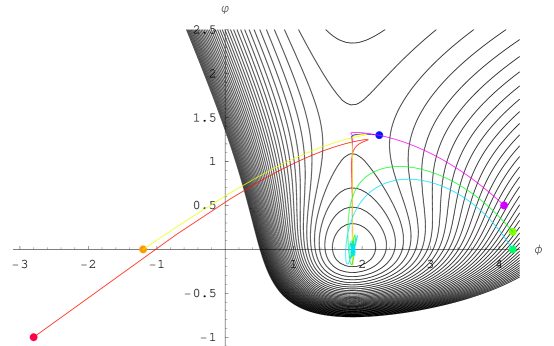
Figure 2: Contour plot of the effective potential $U_{eff}(\varphi,\phi)$ (3.1) with potential $U(\phi)$ of the form (3.7) for parameters $d_{1}=1\,,\xi\Lambda_{D}=1$ and relations $U(\phi_{0})=f_{1}^{2}=\lambda/2$ . This plot clearly shows the global minimum and the saddle. The colored lines describe trajectories for scalar fields starting at different initial conditions.

Let us discuss now a possibility of the external space inflation in this model. It can be easily realized that for all models of the form (3.1) in the case of local zero minimum at $(\varphi=0,\phi_{0})$, the effective potential will also have a saddle point at $(\varphi=\varphi_{max},\,\phi_{0})$ with $\varphi_{max}=\sqrt{(d_{1}+2)/2d_{1}}\ln 3<\varphi_{cr}=1.65$ and the slow-roll parameter $|\eta_{\varphi}|$ in this point cannot be less than 1: $|\eta_{\varphi}|=3d_{1}/(d_{1}+2)\geq 1$. Therefore, such saddles are too steep (in the section $\phi=\phi_{0}$) for the slow-roll and topological inflations However, as we shall see below, a short period of De Sitter-like inflation is possible if we start not precisely at the saddle point but first move in the vicinity of the saddle along the line $\varphi\approx\varphi_{max}$ with subsequent turn into zero minimum along the line $\phi\approx\phi_{0}$. Similar situation happens for trajectories from different regions of the effective potential which can reach this saddle and spend here a some time (moving along the line $\varphi\approx\varphi_{max}$).

Let us consider now regions where the following conditions take place:

$$U(\phi)\gg f_{1}^{2}e^{-2\,\sqrt{\frac{2d_{1}}{d_{1}+2}}\;\varphi}\;,\;\>\lambda e^{-\,\sqrt{\frac{2d_{1}}{d_{1}+2}}\;\varphi}.$$ (3.9)

For the potential (3.7) these regions exist both for negative and positive $\phi$. In the case of positive $\phi$ with $\exp(A\phi)\gg\,\mbox{max}\;\left\{1\,,(8\xi\Lambda_{D})^{1/2}\right\}$ we obtain

$$U_{eff}\approx\frac{1}{8\xi}e^{-\sqrt{q}\;\varphi}e^{\sqrt{q_{1}}\;\phi}\,,$$ (3.10)

where $q$ is defined by Eq. (2.10), $q_{1}:=(2A-B)^{2}=d_{1}^{2}/[(d_{1}+2)(d_{1}+3)]$ and $q>q_{1}$. For potential (3.10) the slow-roll parameters are:

$$\epsilon\approx\eta_{1}\approx\eta_{2}\approx\frac{q}{2}+\frac{q_{1}}{2}\,$$ (3.11)

and satisfy the slow-roll conditions $\epsilon,\eta_{1},\eta_{2}<1$. As far as we know, there are no analytic solutions for such two-scalar-field potential. Anyway, from the form of the potential (3.10) and condition $q>q_{1}$ we can get an estimate $a\approx t^{s}$ with $s\gtrsim 2/q$ (e.g. $2/q=3,2,5/3$ for $d_{1}=1,2,3$, respectively). Thus, in these regions we can get a period of power-law inflation. In spite of a rude character of these estimates, we shall see below that external space scale factors undergo power-law inflation for trajectories passing through these regions.

Now, we investigate dynamical behavior of scalar fields and the external space scale factor in more detail. There are no analytic solutions for considered model. So, we use numerical calculations. To do it, we apply a Mathematica package proposed in KP adjusting it to our models and notations (see Appendix A).

The colored lines on the contour plot of the effective potential in Fig. 2 describe trajectories for scalar fields $\varphi$ and $\phi$ with different initial values (the colored dots). The time evolution of these scalar fields is drawn in Fig. 3. Here, the time $t$ is measured in the Planck times and classical evolution starts at $t=1$. For given initial conditions, scalar fields approach the global minimum of the effective potential along spiral trajectories.

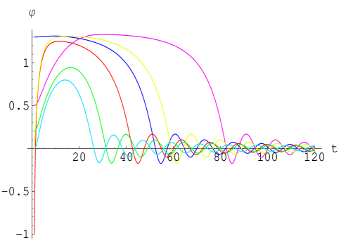
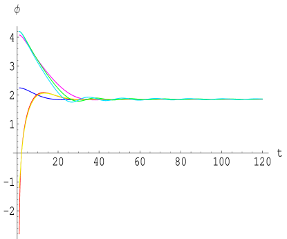
Figure 3: Dynamical behavior of scalar fields $\varphi$ (left panel) and $\phi$ (right panel) with corresponding initial values denoted by the colored dots in Fig. 2.

We plot in Figure 4 the evolution of the logarithms of the scale factor $a(t)$ (left panel) and the evolution of the Hubble parameter $H(t)$ (right panel) and in Fig. 5 the evolution of the parameter of acceleration $q(t)$.

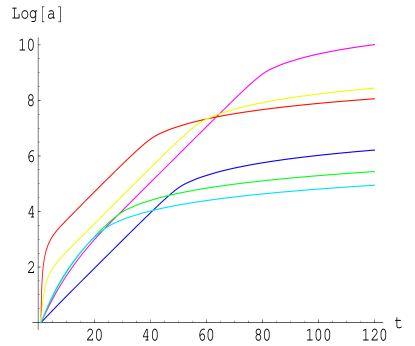
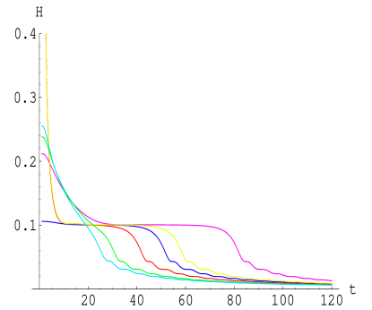
Figure 4: The number of e-folds (left panel) and the Hubble parameter (right panel) for the corresponding trajectories.

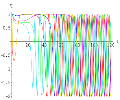
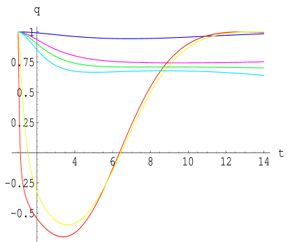
Figure 5: The parameter of acceleration (left panel) and its magnification for early times (right panel). There are two different form of acceleration with $q\approx 1$ (De Sitter-like inflation) and $q\approx 0.75$ (power-law inflation with $s\approx 4$) accordingly. The averaging of $q$ over a few periods of oscillations results in $\bar{q}=-0.5$ which corresponds to the matter dominated decelerating Universe.

Because for initial condition we use the value $a(t=1)=1$ (in the Planck units), then $\log a(t)$ gives the number of e-folds: $\log a(t)=N(t)$. The Figure 4 shows that for considered trajectories we can reach the maximum of e-folds of the order of 10. Clearly, 10 e-folds is not sufficient to solve the horizon and flatness problems but it can be useful to explain a part of the modern CMB data. For example, the Universe inflates by $\triangle N\approx 4$ during the period that wavelengths corresponding to the CMB multipoles $2\leq l\leq 100$ cross the Hubble radius CMB . However, to have the inflation which is long enough for all modes which contribute to the CMB to leave the horizon, it is usually supposed that $\triangle N\geq 15$ WMAP5 .

The Figure 4 for the evolution of the Hubble parameter (right panel) demonstrates that the red, yellow, dark blue and pink lines have a plateau $H\approx const$. It means that the scale factor $a(t)$ has a stage of the De Sitter expansion on these plateaus. Clearly, it happens because these lines reach the vicinity of the effective potential saddle point and spend there some time.

The Fig. 5 for the acceleration parameter defined in (A.9) confirms also the above conclusions. According to Eq. (A.11), $q=1$ for the De Sitter-like behavior. Indeed, all these 4 lines have stages $q\approx 1$ for the same time intervals when $H$ has a plateau. Additionally, the magnification of this picture at early times (the right panel of the Figure 5) shows that pink, green and blue lines have also a period of time when $q$ is approximately constant less than one: $q\approx 0.75$. In accordance with Eq. (A.11), it means that during this time the scale factor $a(t)$ undergoes the power-law inflation $a(t)\propto t^{s}$ with $s\approx 4$. This result confirms our rude estimates made above for the trajectories which go through the regions where the effective potential has the form (3.10). After stages of the inflation, the acceleration parameter starts to oscillate. Averaging $q$ over a few periods of oscillations, we obtain $\bar{q}=-0.5$. Therefore, the scale factor behaves as for the matter dominated Universe: $a(t)\propto t^{2/3}$. Clearly, it corresponds to the times when the trajectories reach the vicinity of the effective potential global minimum and start to oscillate there. It is worth of noting, that there is no need to plot dynamical behavior for the equation of state parameter $\omega(t)$ because it is linearly connected with $q$ (see Eq. (A.10)) and its behavior can be easily understood from the pictures for $q(t)$.

As we have seen above for considered quadratic model, the maximal number of e-folds is near 10. Can we increase this number? To answer this question, we shall consider a new model with a higher degree of nonlinearity, i.e. the nonlinear quartic model.

IV Nonlinear quartic model

In this section we consider the nonlinear quartic model

$$f(\bar{R})=\bar{R}+\gamma\bar{R}^{4}-2\Lambda_{D}\,.$$ (4.1)

For this model the scalar field potential (3.4) reads GZBR :

$$U(\phi)=\frac{1}{2}e^{-B\phi}\left[\frac{3}{4}(4\gamma)^{-1/3}(e^{A\phi}-1)^{4/3}+2\Lambda_{D}\right]\,.$$ (4.2)

Here, the scalar curvature $\bar{R}$ and scalar field $\phi$ are connected as follows: $e^{A\phi}\equiv f^{\prime}=1+4\gamma\bar{R}^{3}\quad\Leftrightarrow\quad\bar{R}=\left[(e^{A\phi}-1)/4\gamma\right]^{1/3}\;.$

We are looking for a solution which has a nonnegative minimum of the effective potential $U_{eff}(\varphi,\phi)$ (3.1) where potential $U(\phi)$ is given by Eq. (4.2). If $\phi_{0}$ corresponds to this minimum, then, as we mentioned above (see also Zhuk ), $U(\phi_{0}),\lambda$ and $f_{1}^{2}$ should be positive. To get zero minimum of the effective potential, these positive values should satisfy the relation of the form of (2.8): $U(\phi_{0})=f_{1}^{2}=\lambda/2$. Additionally, it is important to note that positiveness of $U(\phi_{0})$ results in positive expression for $\bar{R}(\phi_{0})>0$ GZBR .

Eq. (4.2) shows that potential $U(\phi)$ has the following asymptotes for positive $\gamma$ and $\Lambda_{D}$ : $\phi\to-\infty\Longrightarrow U(\phi)\approx\frac{1}{2}e^{-B\phi}\left[\frac{3}{4}(4\gamma)^{-1/3}+2\Lambda_{D}\right]\to+\infty$ and $\phi\to+\infty\Longrightarrow U(\phi)\approx\frac{3}{8}(4\gamma)^{-1/3}e^{(-B+4A/3)\phi}\to+0$. For the latter asymptote we took into account that $-B+4A/3=(D-8)/3\sqrt{(D-2)(D-1)}<0$ for $D<8$. Obviously, the total number of dimensions $D=8$ plays the critical role in quartic nonlinear theories (see GZBR ; BR ; ZhukSaidov2 ) and investigations for $D<8,D=8$ and $D>8$ should be performed separately. To make our paper is not too cumbersome, we consider the case $D<8$ (i.e. $d_{1}=1,2,3$), postponing other cases for our following investigations.

It is worth of noting that for considered signs of parameters, the effective potential $U_{eff}(\varphi,\phi)$ (3.1) acquires negative values when $\phi\to+\infty$ (and $U(\phi)\to 0$). For example, if $U(\phi_{0})=f_{1}^{2}=\lambda/2$ (the case of zero minimum of the effective potential), the effective potential $U_{eff}(\varphi,\phi\to\infty)<0$ for $0<e^{-b\varphi}<2$ and the lowest negative asymptotic value $\left.U_{eff}\right|_{min}\to-(16/27)\lambda$ takes place along the line $e^{-b\varphi}=4/3$. Therefore, zero minimum of $U_{eff}$ is local.

As we mentioned above, extremum positions $\phi_{i}$ of the potential $U(\phi)$ coincide with extremum positions of $U_{eff}(\varphi,\phi)\;:\left.dU/d\phi\right|_{\phi_{i}}=0\to\left.\partial_{\phi}U_{eff}\right|_{\phi_{i}}=0$. The condition of extremum for the potential $U(\phi)$ reads:

$$\frac{dU}{d\phi}=0\;\Longrightarrow\;\bar{R}^{4}-\frac{(2+d_{1})}{\gamma(4-d_{1})}\bar{R}+2\Lambda_{D}\frac{(4+d_{1})}{\gamma(4-d_{1})}=0\,.$$ (4.3)

For positive $\gamma$ and $\Lambda_{D}$ this equation has two real roots:

$$\bar{R}_{0(1)}=\frac{\Lambda_{D}}{2}\left(-\sqrt{\frac{2(2+d_{1})}{(4-d_{1})k\sqrt{M}}-M}+\sqrt{M}\right)\;,$$ (4.4)

$$\bar{R}_{0(2)}=\frac{\Lambda_{D}}{2}\left(\sqrt{\frac{2(2+d_{1})}{(4-d_{1})k\sqrt{M}}-M}+\sqrt{M}\right)\;,$$ (4.5)

where we introduced a dimensionless parameter

$$k:=\gamma\Lambda_{D}^{3}\,,$$ (4.6)

which is positive for positive $\gamma$ and $\Lambda_{D}$, and quantities $M,\;\omega$ read

$$M \equiv -2^{10/3}\frac{(4+d_{1})}{\omega^{1/3}}-\frac{1}{3\cdot 2^{1/3}k}\frac{\omega^{1/3}}{(4-d_{1})}\;,$$ (4.7)

$$\omega \equiv k\left[-27(4-d_{1})(2+d_{1})^{2}\right.$$

$$+ \left.\sqrt{27^{2}(4-d_{1})^{2}(2+d_{1})^{4}-4\cdot 24^{3}k(16-d_{1}^{2})^{3}}\;\right].$$

It can be easily seen that for $k>0$ we get $\omega<0$ and $M\geq 0$. To have real $\omega$, parameter $k$ should satisfy the following condition

$$k\leq\frac{27^{2}(4-d_{1})^{2}(2+d_{1})^{4}}{4\cdot 24^{3}(16-d_{1}^{2})^{3}}\equiv k_{0}\,.$$ (4.9)

It is not difficult to verify that roots $\bar{R}_{0(1,2)}$ are real and positive if $0<k\leq k_{0}$ and they degenerate for $k\to k_{0}\,:\quad\bar{R}_{0(1,2)}\to(\Lambda_{D}/2)\sqrt{M}$. In this limit the minimum and maximum of $U(\phi)$ merge into an inflection point. Now, we should define which of these roots corresponds to minimum of $U(\phi)$ and which to local maximum. The minimum condition

$$\left.\frac{d^{2}U(\phi)}{d\phi^{2}}\right|_{\phi_{0}}>0\;\Longrightarrow\;\gamma\left[(d_{1}+2)-4\gamma\bar{R}_{0}^{3}(4-d_{1})\right]>0$$ (4.10)

results in the following inequality:

$$\gamma>0\;:\quad(d_{1}+2)-4\gamma\bar{R}_{0}^{3}(4-d_{1})>0\,.$$ (4.11)

Thus, the root $\bar{R}_{0}$ which corresponds to the minimum of $U(\phi)$ should satisfy the following condition:

$$0<\bar{R}_{0}<\left(\frac{d_{1}+2}{4\gamma(4-d_{1})}\right)^{1/3}\,.$$ (4.12)

Numerical analysis shows that $\bar{R}_{0(1)}$ satisfies these conditions and corresponds to the minimum. For $\bar{R}_{0(2)}$ we obtain that $\bar{R}_{0(2)}>\left(\frac{d_{1}+2}{4\gamma(4-d_{1})}\right)^{1/3}$ and corresponds to the local maximum of $U(\phi)$. In what follows we shall use the notations:

$$\phi_{min} = \frac{1}{A}\ln\left[1+4\gamma\bar{R}_{0(1)}^{3}\right]\,,$$ (4.13)

$$\phi_{max} = \frac{1}{A}\ln\left[1+4\gamma\bar{R}_{0(2)}^{3}\right]$$ (4.14)

and $U(\phi_{min})\equiv U_{min}\,,U(\phi_{max})\equiv U_{max}$. We should note that $\phi_{min}\,,\phi_{max}$ and the ratio $U_{max}/U_{min}$ depend on the combination $k$ (4.6) rather than on $\gamma$ and $\Lambda_{D}$ taken separately.

Obviously, because potential $U(\phi)$ has two extrema at $\phi_{min}$ and $\phi_{max}$, the effective potential $U_{eff}(\varphi,\phi)$ may have points of extrema only on the lines $\phi=\phi_{min}$ and $\phi=\phi_{max}$ where $\partial U_{eff}/\partial\phi|_{\phi_{min},\phi_{max}}=0$. To find these extrema of $U_{eff}$, it is necessary to consider the second extremum condition $\partial U_{eff}/\partial\varphi=0$ on each line separately:

$$\frac{\partial U_{eff}}{\partial\varphi}=0\Longrightarrow\left\{\begin{array}[]{cc}-U_{min}-3f_{1}^{2}\chi^{2}_{1}+2\lambda\chi_{1}=0\;,\\ \\ -U_{max}-3f_{1}^{2}\chi^{2}_{2}+2\lambda\chi_{2}=0\;,\\ \end{array}\right.$$ (4.15)

where $\chi_{1}\equiv\exp\left(-\sqrt{2d_{1}/(d_{1}+2)}\,\varphi_{1}\right)>0$ and $\chi_{2}\equiv\exp\left(-\sqrt{2d_{1}/(d_{1}+2)}\,\varphi_{2}\right)>0$; $\varphi_{1}$ and $\varphi_{2}$ denote positions of extrema on the lines $\phi=\phi_{min}$ and $\phi=\phi_{max}$, respectively. These equations have solutions

$$\chi_{1(\pm)}=\alpha \pm \sqrt{\alpha^{2}-\beta}\,,$$

$$\alpha \geq \sqrt{\beta}\equiv\alpha_{1}\,;$$ (4.16)

$$\chi_{2(\pm)}=\alpha \pm \sqrt{\alpha^{2}-\beta\frac{U_{max}}{U_{min}}}\,,$$

$$\alpha \geq \sqrt{\beta\frac{U_{max}}{U_{min}}}\equiv\alpha_{2}>\alpha_{1}\,;$$ (4.17)

where we have introduced the notations: $\alpha\equiv\lambda/(3f_{1}^{2})$ and $\beta\equiv U_{min}/(3f_{1}^{2})$. These equations show that there are 5 different possibilities which are listed in the Table 1.

Table 1: The number of extrema of the effective potential $U_{eff}$ depending on the relation between parameters.

$0<\alpha<\alpha_{1}$	$\alpha=\alpha_{1}$	$\alpha_{1}<\alpha<\alpha_{2}$	$\alpha=\alpha_{2}$	$\alpha>\alpha_{2}$
no extrema	one extremum (point of inflection on the line $\phi=\phi_{min}$)	two extrema (one minimum and one saddle on the line $\phi=\phi_{min}$ )	three extrema (minimum and saddle on the line $\phi=\phi_{min}$, inflection on the line $\phi=\phi_{max}$)	four extrema (minimum and saddle on the line $\phi=\phi_{min}$ maximum and saddle on the line $\phi=\phi_{max}$)

To clarify which of solutions (IV) and (IV) correspond to minima of the effective potential (with respect to $\varphi$) we should consider the minimum condition

$$\left.\frac{\partial^{2}U_{eff}}{\partial^{2}\varphi}\right|_{min}>0\quad\Longrightarrow\quad U_{extr}+\chi^{2}9f_{1}^{2}-4\lambda\chi>0\,,$$ (4.18)

where $U_{extr}$ is either $U_{min}$ or $U_{max}$ and $\chi$ denotes either $\chi_{1}$ or $\chi_{2}$. Taking into account relations (4.15), we obtain

$$\chi^{2}3f_{1}^{2}-\chi\lambda>0\quad\Longrightarrow\quad\chi>\frac{\lambda}{3f_{1}^{2}}=\alpha.$$ (4.19)

Thus, roots $\chi_{1,2(+)}$ define the positions of local minima of the effective potential with respect to the variable $\varphi$ and $\chi_{1,2(-)}$ correspond to local maxima (in the direction of $\varphi$).

Now, we fix the minimum $\chi_{1(+)}$ at the point $\varphi=0$. It means that in this local minimum the internal space scale factor is stabilized at the present day value. In this case

$$\left.\chi_{1(+)}\right|_{\varphi=0}=1=\alpha+\sqrt{\alpha^{2}-\beta}\quad\Longrightarrow\quad\alpha=\frac{1+\beta}{2}\,.$$ (4.20)

Obviously, we can do it only if $\alpha<1\Rightarrow\beta\in[0,1)$. For $\chi_{1(-)}$ we get: $\chi_{1(-)}=\beta$.

Additionally, the local minimum of the effective potential at the point $(\varphi=0,\phi=\phi_{min})$ should play the role of the nonnegative four-dimensional effective cosmological constant. Thus, we arrive at the following condition:

$$\Lambda_{eff} \equiv U_{eff}(\varphi=0,\phi=\phi_{min})$$ (4.21)

$$= -\lambda+U_{min}+f_{1}^{2}\geq 0$$

$$\Longrightarrow -\alpha+\beta+\frac{1}{3}\geq 0\,.$$

From the latter inequality and equation (4.20) we get $\beta\in\left[\frac{1}{3},1\right)$. It can be easily seen that $\beta=1/3$ (and, correspondingly, $\alpha=2/3$) results in $\Lambda_{eff}=0$ and we obtain the mentioned above relations: $U_{min}=f_{1}^{2}=\lambda/2$. In general, it is possible to demand that $\Lambda_{eff}$ coincides with the present day dark energy value $10^{-57}\mbox{cm}^{-2}$. However, it leads to very flat local minimum which means the decompactification of the internal space Zhuk . In what follows, we shall mainly consider the case of zero $\Lambda_{eff}$ although all obtained results are trivially generalized to $\Lambda_{eff}=10^{-57}\mbox{cm}^{-2}$.

Summarizing our results, in the most interesting case of $\alpha>\alpha_{2}$ the effective potential has four extrema: local minimum at $\left(\left.\varphi\right|_{\chi_{1(+)}}=0,\phi_{min}\right)$, local maximum at $\left(\varphi|_{\chi_{2(-)}},\phi_{max}\right)$ and two saddle-points at $\left(\varphi|_{\chi_{1(-)}},\phi_{min}\right)$, and $\left(\left.\varphi\right|_{\chi_{2(+)}},\phi_{max}\right)$ (see Fig. 7).

We pay particular attention to the case of zero local minimum $U_{eff}(\left.\varphi\right|_{\chi_{1(+)}}=0,\phi_{min})=0$ where $\beta=1/3\Longrightarrow\alpha=(1+\beta)/2=2/3$. To satisfy the four-extremum condition $\alpha>\alpha_{2}$, we should demand

$$\frac{U_{max}}{U_{min}}<\frac{4}{3}\;.$$ (4.22)

The fraction $U_{max}/U_{min}$ is the function of $k$ and depends parametrically only on the internal space dimension $d_{1}$. Inequality (4.22) provides the lower bound on $k$ and numerical analysis (see Fig. 6)

Figure 6: The form of $U_{max}/U_{min}$ as a function of $k\in(0,k_{0}]$ for $d_{1}=1,2,3$ from left to right, respectively. Dashed line corresponds to $U_{max}/U_{min}=4/3$.

gives $\tilde{k}(d_{1}=1)\approx 0.000625\;;\;\tilde{k}(d_{1}=2)\approx 0.00207\;;\;\tilde{k}(d_{1}=3)\approx 0.0035\,.$ Therefore, effective potentials with zero local minimum will have four extrema if $k\in(\tilde{k},k_{0})$ (where $k_{0}$ is defined by Eq. (4.9)). The limit $k\to\tilde{k}$ results in merging $\chi_{2(-)}\leftrightarrow\chi_{2(+)}$ and the limit $k\to k_{0}$ results in merging $\chi_{1(-)}\leftrightarrow\chi_{2(-)}$ and $\chi_{1(+)}\leftrightarrow\chi_{2(+)}$. Such merging results in transformation of corresponding extrema into inflection points. For example, from Fig. 6 follows that $U_{max}/U_{min}\to 1$ for $k\to k_{0}$.

The typical contour plot of the effective potential with four extrema in the case of zero local minimum is drawn in Fig. 7. Here, for $d_{1}=3$ we take $k=0.004\in(\tilde{k},k_{0})$ which gives $\alpha_{2}\approx 0.655$. Thus, $\alpha=2/3\approx 0.666>\alpha_{2}$.

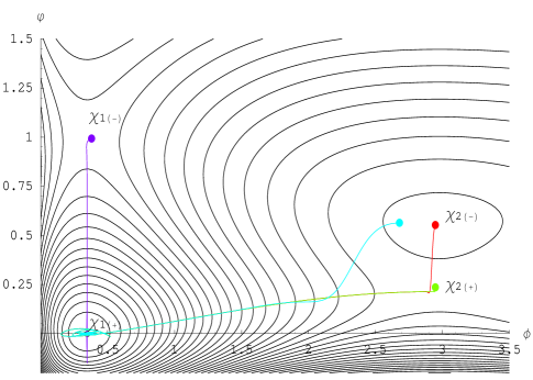
Figure 7: Contour plot of the effective potential $U_{eff}(\varphi,\phi)$ (3.1) with potential $U(\phi)$ of the form (4.2) for parameters $\beta=1/3$, $d_{1}=3$ and $k=0.004$. This plot shows the local zero minimum, local maximum and two saddles. The colored lines describe trajectories for scalar fields starting at different initial conditions.

Let us investigate now a possibility of inflation for considered potential. First of all, taking into account the comments in previous section (see a paragraph before Eq. (3.9)), it is clear that topological inflation in the saddle point $\chi_{1(-)}$ as well as the slow rolling from there in the direction of the local minimum $\chi_{1(+)}$ are absent. It is not difficult to verified that the generalized power-low inflation discussed in the case of the nonlinear quadratic model is also absent here. Indeed, from Eqs. (3.1) and (4.2) follows that nonlinear potential $U(\phi)$ can play the leading role in the region $\phi\to-\infty$ (because $U(\phi)\to 0$ for $\phi\to+\infty$). In this region $U_{eff}\propto\exp{(-\sqrt{q}\varphi)}\exp{(-\sqrt{q_{2}}\phi)}$ where $q=2d_{1}/(d_{1}+2)$ and $q_{2}=B^{2}=(d_{1}+4)^{2}/[(d_{1}+2)(d_{1}+3)]$. For these values of $q$ and $q_{2}$ the slow-roll conditions are not satisfied: $\epsilon\approx\eta_{1}\approx\eta_{2}\approx{q}/{2}+{q_{2}}/{2}>1$. However, there are two promising regions where the stage of inflation with subsequent stable compactification of the internal space may take place. We mean the local maximum $\chi_{2(-)}$ and the saddle $\chi_{2(+)}$ (see Fig. 7). Let us estimate the slow roll parameters for these regions.

We consider first the local maximum $\chi_{2(-)}$. It is obvious that the parameter $\epsilon$ is equal to zero here. Additionally, from the form of the effective potential (3.1) it is clear that the mixed second derivatives are also absent in extremum points. Thus, the slow roll parameters $\eta_{1}$ and $\eta_{2}$, defined in the footnote (8), coincide exactly with $\eta_{\varphi}$ and $\eta_{\phi}$. In Fig. 8 we present typical form of these parameters as functions of $k\in(\tilde{k},k_{0})$ in the case $\beta=1/3$ and $d_{1}=1,2,3$.

Figure 8: Graphs of $|\eta_{\varphi}|$ (left panel) and $|\eta_{\phi}|$ (right panel) as functions of $k\in(\tilde{k},k_{0})$ for local maximum $\chi_{2(-)}$ and parameters $\beta=1/3$ and $d_{1}=1,2,3$.

These plots show that, for considered parameters, the slow roll inflation in this region is possible for $d_{1}=1,3$.

The vicinity of the saddle point $\chi_{2(+)}$ is another promising region. Obviously, if we start from this point, a test particle will roll mainly along direction of $\phi$. That is why it makes sense to draw only $|\eta_{\phi}|$. In Fig. 9 we plot typical form of $|\eta_{\phi}|$ in the case $\beta=1/3$ and $d_{1}=1,2,3$. Left panel represents general behavior for the whole range of $k\in(\tilde{k},k_{0})$ and right panel shows detailed behavior in the most interesting region of small $k$. It shows that $d_{1}=3$ is the most promising case in this region.

Figure 9: Grafs of $|\eta_{\phi}|$ as functions of $k$ for saddle point $\chi_{2(+)}$ and parameters $\beta=1/3$ and $d_{1}=1,2,3$. Left panel demonstrates the whole region of variable $k\in(\tilde{k},k_{0})$ and right panel shows detailed behavior for small $k$.

Now, we investigate numerically the dynamical behavior of scalar fields and the external space scale factor for trajectories which start from the regions $\chi_{1(-)},\chi_{2(-)}$ and $\chi_{2(+)}$. All numerical calculations perform for $\beta=1/3,d_{1}=3$ and $k=0.004$. The colored lines on the contour plot of the effective potential in Fig. 7 describe trajectories for scalar fields $\varphi$ and $\phi$ with different initial values (the colored dots) in the vicinity of these extrema points. The time evolution of these scalar fields is drawn in Fig. 10. For given initial conditions, scalar fields approach the local minimum $\chi_{1(+)}$ of the effective potential along the spiral trajectories.

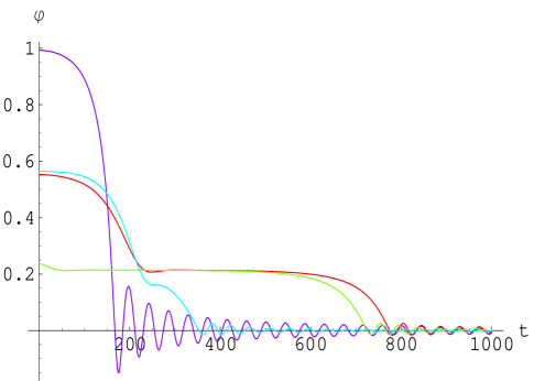
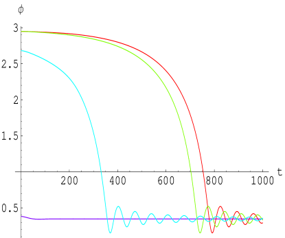
Figure 10: Dynamical behavior of scalar fields $\varphi$ (left panel) and $\phi$ (right panel) with corresponding initial values denoted by the colored dots in Fig. 7.

We plot in Figure 11 the evolution of the logarithm of the scale factor $a(t)$ (left panel) which gives directly the number of e-folds and the evolution of the Hubble parameter $H(t)$ (right panel) and in Fig. 12 the evolution of the parameter of acceleration $q(t)$.

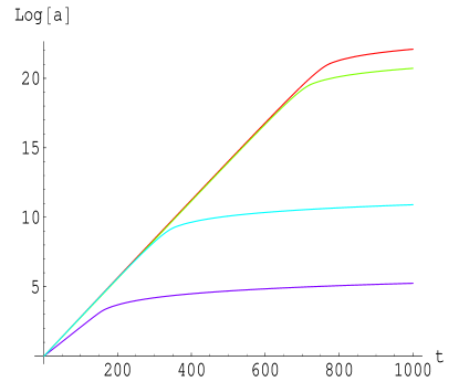
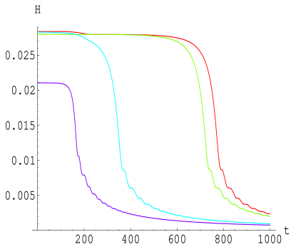
Figure 11: The number of e-folds (left panel) and the Hubble parameter (right panel) for the corresponding trajectories.

Figure 12: The parameter of acceleration (left panel) and its magnification for early times (right panel).

The Figure 11 shows that for considered trajectories we can reach the maximum of e-folds of the order of 22 which is long enough for all modes which contribute to the CMB to leave the horizon.

The Figure 11 for the evolution of the Hubble parameter (right panel) demonstrates that all lines have plateaus $H\approx const$. However, the red, yellow and blue lines which pass in the vicinity of the saddle $\chi_{2(+)}$ have bigger value of the Hubble parameter with respect to the dark blue line which starts from the $\chi_{1(-)}$ region. Therefore, the scale factor $a(t)$ has stages of the De Sitter-like expansion corresponding to these plateaus which last approximately from 100 (dark blue line) up to 800 (red line) Planck times.

The Fig. 12 for the acceleration parameter confirms also the above conclusions. All 4 lines have stages $q\approx 1$ for the same time intervals when $H$ has plateaus. After stages of inflation, the acceleration parameter starts to oscillate. Averaging $q$ over a few periods of oscillations, we obtain $\bar{q}=-0.5$. Therefore, the scale factor behaves as for the matter dominated Universe: $a(t)\propto t^{2/3}$. Clearly, it corresponds to the times when the trajectories reach the vicinity of the effective potential local minimum $\chi_{1(+)}$ and start to oscillate there.

Let us investigate now a possibility of the topological inflation Linde ; Vilenkin if scalar fields $\varphi,\phi$ stay in the vicinity of the saddle point $\chi_{2(+)}$. As we mentioned in Section 2, topological inflation in the case of the double-well potential takes place if the distance between a minimum and local maximum bigger than $\Delta\phi_{cr}=1.65$. In this case domain wall is thick enough in comparison with the Hubble radius. The critical ratio of the characteristic thickness of the wall to the horizon scale in local maximum is $r_{w}H\approx|U/3\partial U_{\phi\phi}|^{1/2}\approx 0.48$ SSTM and for topological inflation it is necessary to exceed this critical value. Therefore, we should cheque the saddle $\chi_{2(+)}$ from the point of these criteria.

In Fig. 13 (left panel) we draw the difference $\Delta\phi=\phi_{max}-\phi_{min}$ for the profile $\varphi=\varphi|_{\chi_{2(+)}}$ as a functions of $k\in(\tilde{k},k_{0})$ in the case $\beta=1/3$ for dimensions $d_{1}=1,2,3$. This picture shows that this difference can exceed the critical value if the number of the internal dimensions is $d_{1}=2$ and $d_{1}=3$. Right panel of Fig. 13 confirms this conclusion. Here we consider the case $\beta=1/3,\quad k=0.004$ and $d_{1}=3$. For chosen values of the parameters, $\Delta\phi=2.63$ which is considerably bigger than the critical value 1.65 and the ratio of the thickness of the wall to the horizon scale is 1.30 which again bigger than the critical value 0.48. Therefore, topological inflation can happen for considered model. Moreover, due to quantum fluctuations of scalar fields, inflating domain wall will have fractal structure: it will contain many other inflating domain walls and each of these domain walls again will contain new inflating domain walls and so on Linde . Thus, from this point, such topological inflation is the eternal one.

Figure 13: Left panel demonstrates the difference $\phi_{max}-\phi_{min}$ (for the profile $\varphi=\varphi|_{\chi_{2(+)}}$) as a functions of $k\in(\tilde{k},k_{0})$ for parameters $\beta=1/3$, and $d_{1}=1,2,3$ (from left to right respectively). Dashed line corresponds to $\phi_{max}-\phi_{min}=1.65$. Right panel shows the comparison of the potential $U_{eff}(\varphi|_{\chi_{2(+)}},\phi)$ with a double-well potential for parameters $\beta=1/3,k=0.004$ and $d_{1}=3$.

To conclude this section, we want to draw the attention to one interesting feature of the given model. From above consideration follows that in the case of zero minimum of the effective potential the positions of extrema are fully determined by the parameters $k$ and $d_{1}$, and for fixed $k$ and $d_{1}$ do not depend on the choice of $\Lambda_{D}$. The same takes place for the slow roll parameters. On the other hand, if we keep $k$ and $d_{1}$, the hight of the effective potential is defined by $\Lambda_{D}$ (see Appendix B). Therefore, we can change the hight of extrema with the help of $\Lambda_{D}$ but preserve the conditions of inflation for given $k$ and $d_{1}$.

However, the dynamical characteristics of the model (drawn in figures 10 - 12) depend on variations of $\Lambda_{D}$ by the self-similar manner. It means that the change of hight of the effective potential via transformation $\Lambda_{D}\to c\Lambda_{D}$ ($c$ is a constant) with fixed $k$ and $d_{1}$ results in rescaling of figures 10 - 12 in $1/\sqrt{c}$ times along the time axis.

V Summary and discussion

In our paper we investigated a possibility of inflation in multidimensional cosmological models. The main attention was paid to nonlinear (in scalar curvature) models with quadratic $R^{2}$ and quartic $R^{4}$ lagrangians. These models contain two scalar fields. One of them corresponds to the scale factor of the internal space and another one is related with the nonlinearity of the original models. The effective four-dimensional potentials in these models are fully determined by the geometry and matter content of the models. The geometry is defined by the direct product of the Ricci-flat external and internal spaces. As a matter source, we include a monopole form field, D-dimensional bare cosmological constant and tensions of branes located in fixed points. The exact form of the effective potentials depends on the relation between parameters of the models and can take rather complicated view with a number of extrema points.

First of all, we found a range of parameters which insures the existence of zero minima of the effective potentials. These minima provide sufficient condition to stabilize the internal space and, consequently, to avoid the problem of the fundamental constant variation. Zero minima correspond to the zero effective four-dimensional cosmological constant. In general, we can also consider positive effective cosmological constant which corresponds to the observable now dark energy. However, it usually requires extreme fine tuning of parameters of models.

Then, for corresponding effective potentials, we investigated the possibility of the external space inflation. We have shown that for some initial conditions in the quadratic and quartic models we can achieve up to 10 and 22 e-folds, respectively. An additionally bonus of the considered model is that $R^{4}$ model can provide conditions for the eternal topological inflation.

Obviously, 10 and 22 e-folds are not sufficient to solve the homogeneity and isotropy problem but big enough to explain the recent CMB data. To have the inflation which is long enough for modes which contribute to the CMB, it is usually supposed that $\triangle N\geq 15$ WMAP5 . Moreover, 22 e-folds is rather big number to encourage the following investigations of the nonlinear multidimensional models to find theories where this number will approach 50-60. We have seen that the increase of the nonlinearity (from quadratic to quartic one) results in the increase of $\triangle N$ in more that two times. So, there is a hope that more complicated nonlinear models can provide necessary 50-60 e-folds. Besides, this number is reduced in models where long matter dominated (MD) stage followed inflation can subsequently decay into radiation LiddleLyth ; BV . Precisely this scenario takes place for our models. We have shown for quadratic and quartic nonlinear models, that MD stage with the external scale factor $a\sim t^{2/3}$ takes place after the stage of inflation. It happens when scalar fields start to oscillate near the position of zero minimum of the effective potential. However, scalar fields are not stable. For example, scalar field $\varphi$ decays into two photons $\varphi\to 2\gamma$ with the decay rate $\Gamma\sim m_{\varphi}^{3}/M_{Pl}^{2}$ GSZ . Thus the life time is $\tau_{decay}\sim(M_{Pl}/m_{\varphi})^{3}t_{Pl}$. The reheating temperature is given by the expression $T_{RH}\sim(m_{\varphi}^{3}/M_{Pl})^{1/2}$. Therefore, to get $T_{RH}\gtrsim 1$MeV necessary for the nucleosynthesis, we should take $m_{\varphi}\gtrsim 10$TeV. In paper BV , it is shown that for such scenario with intermediate MD stage, the necessary number of e-folds is reduced according to the formula:

$$\triangle N = -\frac{1}{6}\ln\left(\frac{45}{2}g^{-3/2}_{*}\frac{m_{\varphi}^{2}}{\Gamma M_{Pl}}\right)$$ (5.1)

$$= -\frac{1}{6}\ln\left(\frac{45}{2}g^{-3/2}_{*}\frac{M_{Pl}}{m_{\varphi}}\right)\,,$$

where $g_{*}$ counts the effective number of relativistic degrees of freedom and we took into account that decaying particles are scalars. This expression weakly depends on $g_{*}$. For example, if $m_{\varphi}\sim 10$TeV we obtain $-6.27\leq\triangle N\leq-5.11$ for $1\leq g_{*}\leq 10^{2}$. Thus, $\triangle N\approx-6$. Therefore, we believe that the number of e-folds is not a big problem for multidimensional nonlinear models. The main problem consists in the spectral index. For example, in the case of $R^{4}$ model we get $n_{s}\approx 1+2\eta|_{\chi_{2(+)}}\approx 0.61$ which is less than observable now $n_{s}\approx 1$. A possible solution of this problem may consist in more general form of the nonlinearity $f(R)$. It was observed in Ellis that simultaneous consideration quadratic and quartic nonlinearities can flatten the effective potential and increase $n_{s}$. We postpone this problem for our following investigations.

Appendix A Friedmann equations for multi-component scalar field model

We consider $n$ scalar fields minimally coupled to gravity in four dimensions. The effective action of this model reads

$$S =\frac{1}{16\pi G}\int d^{4}x\sqrt{|\tilde{g}^{(0)}|}\left(R[\tilde{g}^{(0)}]\right.$$ (A.1)

$$- \left.G_{ij}\tilde{g}^{(0)\mu\nu}\partial_{\mu}\varphi^{i}\partial_{\nu}\varphi^{j}-2U(\varphi^{1},\varphi^{2},\ldots)\right)$$

where the kinetic term is usually taken in the canonical form: $G_{ij}=\mbox{diag}(1,1,\ldots)$ (flat $\sigma$ model). Such multi-component scalar fields originate naturally in multidimensional cosmological models (with linear or nonlinear gravitational actions) GZ1 ; GZ2 ; GMZ1 . We use the usual conventions $c=\hbar=1$, i.e. $L_{Pl}=t_{Pl}=1/M_{Pl}$ and $8\pi G=8\pi/M^{2}_{Pl}$. Here, scalar fields are dimensionless and potential $U$ has dimension $[U]=\mbox{lehgth}^{-2}$.

Because we want to investigate dynamical behavior of our Universe in the presence of scalar fields, we suppose that scalar fields are homogeneous: $\varphi^{i}=\varphi^{i}(t)$ and four-dimensional metric is spatially-flat Friedmann-Robertson-Walker one: $\tilde{g}^{(0)}=-dt\otimes dt+a^{2}(t)d\vec{x}\otimes d\vec{x}$.

For energy density and pressure we easily get:

$$\rho = \frac{1}{8\pi G}\left(\frac{1}{2}G_{ij}\dot{\varphi}^{i}\dot{\varphi}^{j}+U\right)\,,$$

$$P = \frac{1}{8\pi G}\left(\frac{1}{2}G_{ij}\dot{\varphi}^{i}\dot{\varphi}^{j}-U\right)\,;$$ (A.2)

$$\Longrightarrow \left\{\begin{array}[]{ll}\frac{1}{2}G_{ij}\dot{\varphi}^{i}\dot{\varphi}^{j}=4\pi G(\rho+P)\;,\\ \\ U=4\pi G(\rho-P)\;.\end{array}\right.$$ (A.6)

The Friedmann equations for considered model are

$$3\left(\frac{\dot{a}}{a}\right)^{2}\equiv 3H^{2}=8\pi G\rho=\frac{1}{2}G_{ij}\dot{\varphi}^{i}\dot{\varphi}^{j}+U\,,$$ (A.7)

and

$$\dot{H}=-4\pi G(\rho+P)=-\frac{1}{2}G_{ij}\dot{\varphi}^{i}\dot{\varphi}^{j}\,.$$ (A.8)

From these 2 equations, we obtain the following expression for the acceleration parameter:

$$q \equiv \frac{\ddot{a}}{H^{2}a}=1-\frac{4\pi G}{H^{2}}(\rho+P)=-\frac{8\pi G}{6H^{2}}(\rho+3P)$$ (A.9)

$$= \frac{1}{6H^{2}}\left(-4\times\frac{1}{2}G_{ij}\dot{\varphi}^{i}\dot{\varphi}^{j}+2U\right)\,.$$

It can be easily seen that the equation of state (EoS) parameter $\omega=P/\rho$ and parameter $q$ are linearly connected:

$$q=-\frac{1}{2}(1+3\omega)\,.$$ (A.10)

From the definition of the acceleration parameter, it follows that $q$ is constant in the case of the power-law and De Sitter-like behavior:

$$q=\left\{\begin{array}[]{cc}(s-1)/s\;;\quad a\propto t^{s}\,,\\ 1\;;\quad a\propto e^{Ht}\,.\\ \end{array}\right.$$ (A.11)

For example, $q=-0.5$ during the matter dominated (MD) stage where $s=2/3$.

Because the minisuperspace metric $G_{ij}$ is flat, the scalar field equations are:

$$\ddot{\varphi}^{i}+3H\dot{\varphi}^{i}+G^{ij}\frac{\partial U}{\partial\varphi^{j}}=0\,.$$ (A.12)

For the action (A.1), the corresponding Hamiltonian is

$$\mathcal{H}=\frac{8\pi G}{2a^{3}}G^{ij}P_{i}P_{j}+\frac{a^{3}}{8\pi G}U\,,$$ (A.13)

where

$$P_{i}=\frac{a^{3}}{8\pi G}G_{ij}\dot{\varphi}^{j}\,$$ (A.14)

are the canonical momenta and equations of motion have also the canonical form

$$\dot{\varphi}^{i}=\frac{\partial\mathcal{H}}{\partial P_{i}}\,,\quad\dot{P}_{i}=-\frac{\partial\mathcal{H}}{\partial\varphi^{i}}\,.$$ (A.15)

It can be easily seen that the latter equation (for $\dot{P}_{i}$) is equivalent to the eq. (A.12).

Thus, the Friedmann equations together with the scalar field equations can be replaced by the system of the first order ODEs:

$$\dot{\varphi}^{i} =\frac{8\pi G}{a^{3}}G^{ij}P_{j}\,,$$ (A.16)

$$\dot{P}_{i} =-\frac{a^{3}}{8\pi G}\frac{\partial U}{\partial\varphi^{i}}\,,$$ (A.17)

$$\dot{a} =aH\,,$$ (A.19)

$$\dot{H} =\frac{\ddot{a}}{a}-H^{2}$$

$$=\frac{1}{6}\left(-4\times\frac{1}{2}G_{ij}\dot{\varphi}^{i}\dot{\varphi}^{j}+2U\right)-H^{2}\,$$

with Eq. (A.7) considered in the form of the initial conditions:

$$H(t=0)=\left.\sqrt{\frac{1}{3}\left(\frac{1}{2}G_{ij}\dot{\varphi}^{i}\dot{\varphi}^{j}+U\right)}\;\right|_{t=0}\,.$$ (A.20)

We can make these equations dimensionless:

$$\frac{d\varphi^{i}}{M_{Pl}dt} = \frac{8\pi}{M^{3}_{Pl}a^{3}}G^{ij}P_{j},$$

$$\Rightarrow\frac{d\varphi^{i}}{dt} = \frac{8\pi}{a^{3}}G^{ij}P_{j}\,;$$ (A.21)

$$\frac{dP_{i}}{M_{Pl}dt} = -\frac{a^{3}M^{3}_{Pl}}{8\pi}\frac{\partial(U/M^{2}_{Pl})}{\partial\varphi^{i}}\,,$$

$$\Rightarrow\frac{dP_{i}}{dt} = -\frac{a^{3}}{8\pi}\frac{\partial U}{\partial\varphi^{i}}\,.$$ (A.22)

That is to say the time $t$ is measured in the Planck times $t_{Pl}$, the scale factor $a$ is measured in the Planck lengths $L_{Pl}$ and the potential $U$ is measured in the $M^{2}_{Pl}$ units.

We use this system of dimensionless first order ODEs together with the initial condition (A.20) for numerical calculation of the dynamics of considered models with the help of a Mathematica package KP .

*

Appendix B: Self-similarity condition

Due to the zero minimum conditions $U(\phi_{min})=f_{1}^{2}=\lambda/2$, the effective potential (3.1) can be written in the form:

$$U_{eff}(\varphi,\phi)=U(\phi_{min})e^{-\,\sqrt{\frac{2d_{1}}{d_{1}+2}}\;\varphi}$$

$$\times\left[\frac{U(\phi)}{U(\phi_{min})}+e^{-2\,\sqrt{\frac{2d_{1}}{d_{1}+2}}\;\varphi}-2e^{-\,\sqrt{\frac{2d_{1}}{d_{1}+2}}\;\varphi}\right]\;.\qquad$$ (B.1)

Exact expressions for $U(\phi)$ (3.7) and (4.2) indicate that the ratio

$$\frac{U(\phi)}{U(\phi_{min})}=F(\phi,k,d_{1})$$ (B.2)

depends only on $\phi,k$ and $d_{1}$. Dimensionless parameter $k=\xi\Lambda_{D}$ for the quadratic model and $k=\gamma\Lambda_{D}^{3}$ for the quartic model. In Eq. (B.2) we take into account that $\phi_{min}$ is a function of $k$ and $d_{1}$: $\phi_{min}=\phi_{min}(k,d_{1})$. Then, $U(\phi_{min})$ defined in Eqs. (3.7) and (4.2) reads:

$$U(\phi_{min})=\Lambda_{D}\tilde{F}(\phi_{min}(k,d_{1}),k,d_{1})\,.$$ (B.3)

Therefore, parameters $k$ and $d_{1}$ determine fully the shape of the effective potential, and parameter $\Lambda_{D}$ serves for conformal transformation of this shape. This conclusion is confirmed also in sections 3 and 4 where we show that positions of all extrema depend only on $k$ and $d_{1}$. Thus, figures 2, and 7 for contour plots are defined by $k$ and $d_{1}$ and will not change with $\Lambda_{D}$. From the definition of the slow roll parameters it is clear that they also do not depend on the hight of potentials and in our model depend only on $k$ and $d_{1}$ (see figures 8 and 9). Similar dependence takes place for difference $\Delta\phi=\phi_{max}-\phi_{min}$ drawn in Fig. 13. Thus the conclusions concerning the slow roll and topological inflations are fully determined by the choice of $k$ and $d_{1}$ and do not depend on the hight of the effective potential, in other words, on $\Lambda_{D}$. So, for fixed $k$ and $d_{1}$ parameter $\Lambda_{D}$ can be arbitrary. For example, we can take $\Lambda_{D}$ in such a way that the hight of the saddle point $\chi_{2(+)}$ will correspond to the restriction on the slow roll inflation potential (see e.g. Lyth ) $U_{eff}\lesssim 2.2\times 10^{-11}M_{Pl}^{4}$, or in our notations $U_{eff}\lesssim 5.5\times 10^{-10}M_{Pl}^{2}$.

Above, we indicate figures which (for given $k$ and $d_{1}$) do not depend on the hight of the effective potential (on $\Lambda_{D}$). What will happen with dynamical characteristics drawn in figures 10, 11 and 12 (and analogous ones for the quadratic model) if we, keeping fixed $k$ and $d_{1}$, will change $\Lambda_{D}$? In other words, we keep the positions of the extrema points (in $(\varphi,\phi)$-plane) but change the hight of extrema. We can easily answer this question using the self-similarity condition of the Friedmann equations. Let the potential $U$ in Eqs. (A) and (A.6) be transformed conformally: $U\to c\,U$ where $c$ is a constant. Next, we can introduce a new time variable $\tau:=\sqrt{c}\,t$. Then, from Eqs. (A)-(A.8) follows that the Friedmann equations have the same form as for the model with potential $U$ where time $t$ is replaced by time $\tau$. This condition we call the self-similarity. Thus, if in our model we change the parameter $\Lambda_{D}:\;\Lambda_{D}\to c\,\Lambda_{D}$, it results (for fixed $k$ and $d_{1}$) in rescaling of all dynamical graphics (e.g. Figures 10 - 12) along the time axis in $1/\sqrt{c}$ times (the decrease of $\Lambda_{D}$ leads to the stretch of these figures along the time axis and vice versa the increase of $\Lambda_{D}$ results in the shrink of these graphics). Numerical calculations confirm this conclusion. The property of the conformal transformation of the shape of $U_{eff}$ with change of $\Lambda_{D}$ for fixed $k$ and $d_{1}$ can be also called as the self-similarity.

References

- (1) H.V.Peiris et al., Astrophys.J.Suppl. 148 (2003) 213, arXiv:astro-ph/0302225.
- (2) M. Rainer and A. Zhuk, Gen.Rel.Grav. 32 (2000) 79, arXiv:gr-qc/9808073.
- (3) U. Günther and A. Zhuk, Phys. Rev. D56 (1997) 6391, arXiv:gr-qc/9706050v2.
- (4) R. Kallosh, N. Sivanandam and M. Soroush, Phys. Rev. D 77 (2008) 043501, arXiv:0710.3429.
- (5) A. Linde and A, Westphal, JCAP 0803 (2008) 005, arXiv:0712.1610.
- (6) J. P. Conlon, R. Kallosh, A. Linde and F. Quevedo, Volume Modulus Inflation and the Gravitino Mass Problem, arXiv:0806.0809.
- (7) U. Günther and A. Zhuk, Phys. Rev. D61 (2000) 124001, arXiv:hep-ph/0002009.
- (8) T. P. Sotiriou and V. Faraoni, f(R) Theories Of Gravity, arXiv:0805.1726.
- (9) R. P. Woodard, Lect. Notes Phys., 720 (2007) 403, arXiv:gr-qc/0602110.
- (10) S. Nojiri, S. D. Odintsov, Dark energy, inflation and dark matter from modified F(R) gravity, arXiv:0807.0685.
- (11) U. Günther, A. Zhuk, V.B. Bezerra and C. Romero, Class. Quant. Grav. 22 (2005) 3135, arXiv:hep-th/0409112.
- (12) A.A. Starobinsky, Phys. Lett. B91 (1980) 99.
- (13) U. Günther, P. Moniz and A. Zhuk, Phys. Rev. D66 (2002) 044014, arXiv:hep-th/0205148.
- (14) K.A. Bronnikov and S.G. Rubin, Abilities of multidimensional gravity, Grav and Cosmol. Vol.13, No.4 (2007) 253, arXiv:0712.0888.
- (15) J. Ellis, N. Kaloper, K. A. Olive and J. Yokoyama, Phys.Rev. D59 (1999) 103503, arXiv:hep-ph/9807482.
- (16) A. Linde, Phys.Lett. B327 (1994) 208, arXiv:astro-ph/9402031
- (17) T. Appelquist, H.-C. Cheng and B. A. Dobrescu, Phys.Rev. D64 (2001) 035002, arXiv:hep-ph/0012100; E. Ponton and E. Poppitz, JHEP 0106 (2001) 019, arXiv:hep-ph/0105021; H.-C. Cheng, K. T. Matchev and M. Schmaltz, Phys.Rev. D66 (2002) 036005, arXiv:hep-ph/0204342; G. Servant and T. M.P. Tait, Nucl.Phys. B650 (2003) 391, arXiv:hep-ph/0206071; L. Bergstrom, T. Bringmann, M. Eriksson and M. Gustafsson, Phys.Rev.Lett. 94 (2005) 131301, arXiv:astro-ph/0410359; F. De Fazio, Constraining Universal Extra Dimensions through B decays, arXiv:hep-ph/0609134.
- (18) P.K. Townsend, Four lectures on M-theory, arXiv:hep-th/9612121; J.W. Moffat, M-theory on a supermanifold, arXiv:hep-th/0111225.
- (19) A. Kundu, Universal Extra Dimension, arXiv:0806.3815.
- (20) P.G.O. Freund and M.A. Rubin, Phys. Lett. B97 (1980) 233.
- (21) U. Günther, P. Moniz and A. Zhuk, Phys. Rev. D68 (2003) 044010, arXiv:hep-th/0303023 .
- (22) A. Zhuk, Conventional cosmology from multidimensional models, Proceedings of the 14th International Seminar on High Energy Physics ”QUARKS-2006” in St. Petersburg, May 19-25 2006, vol.2, p.264, INR press, 2007, arXiv:hep-th/0609126.
- (23) B.Ratra and P.J. Peebles, Phys. Rev. D37 (1988) 3406.
- (24) G.F.R. Ellis and M.S. Madsen, Class. Quant. Grav. 8 (1991) 667, .
- (25) B. Ratra, Phys. Rev. D45 (1992) 1913.
- (26) C. Stornaiolo, Phys. Let.A 189 (1994) 351.
- (27) N. Sakai, H. Shinkai, T. Tachizawa and K. Maeda, Phys.Rev. D53 (1996) 655; Erratum-ibid. D54 (1996) 2981, arXiv:gr-qc/9506068.
- (28) T. Saidov and A. Zhuk, Phys. Rev. D75 (2007) 084037, arXiv:hep-th/0612217.
- (29) N. Arkani-Hamed, S. Dimopoulos, J. March-Russell, Phys.Rev. D63 (2001) 064020, arXiv:hep-th/9809124v2.
- (30) U. Günther, A. Starobinsky and A. Zhuk, Phys. Rev. D69 (2004) 044003, arXiv:hep-ph/0306191 .
- (31) Y. M. Cho and Y. Y. Keum, Class. Quant. Grav. 15 (1998) 907.
- (32) Y. M. Cho and J. H. Kim, Dilaton as a Dark Matter Candidate and its Detection, arXiv:0711.2858.
- (33) J. Martin, D. Schwarz, Phys.Rev. D62 (2000) 103520, arXiv:astro-ph/9911225.
- (34) N. Deruelle, M. Sasaki and Y. Sendouda, ”Detuned” f(R) gravity and dark energy, arXiv:0803.2742.
- (35) T.T. Nakamura and E.D. Stewart, Phys. Lett. B 381 (1996) 413, arXiv:astro-ph/9604103; J.-O. Gong and E.D. Stewart, Phys. Lett. B 538 (2002) 213, arXiv:astro-ph/0202098.
- (36) R. Kallosh and S. Prokushkin, SuperCosmology, arXiv:hep-th/0403060.
- (37) D.H. Lyth and A. Riotto, Phys.Rept. 314 (1999) 1, arXiv:hep-ph/9807278; G. Efstathiou, K.J. Mack, JCAP 0505 (2005) 008, arXiv:astro-ph/0503360.
- (38) H. V. Peiris and R. Easther, Primordial Black Holes, Eternal Inflation, and the Inflationary Parameter Space after WMAP5, arXiv:0805.2154.
- (39) T. Saidov and A. Zhuk, Gravitation & Cosmology, 12 (2006) 253, arXiv:hep-th/0604131.
- (40) Alexander Vilenkin, Phys.Rev.Lett. 72 (1994), arXiv:hep-th/9402085.
- (41) D.H. Lyth, Phys.Lett. B147 (1984) 403.
- (42) A.R. Liddle and D. H. Lyth, Phys.Rept. 231 (1993) 1, arXiv:astro-ph/9303019.
- (43) G. Barenboim and O. Vives, About a (standard model) universe dominated by the right matter, arXiv:0806.4389.