The finite-temperature phase structure
of lattice QCD with twisted-mass Wilson fermions

Abstract:

We report progress in our exploration of the finite-temperature phase structure of two-flavour lattice QCD with twisted-mass Wilson fermions and a tree-level Symanzik-improved gauge action for a temporal lattice size $N_{\tau}=8$. Extending our investigations to a wider region of parameter space we gain a global view of the rich phase structure. We identify the finite temperature transition/crossover for a non-vanishing twisted-mass parameter in the neighbourhood of the zero-temperature critical line at sufficiently high $\beta$. Our findings are consistent with Creutz’s conjecture of a conical shape of the finite temperature transition surface. Comparing with NLO lattice $\chi{\rm PT}$ we achieve an improved understanding of this shape.

DESY 08-134   HU-EP-08/40   MS-TP-08-20   SFB/CPP-08-77

1 Introduction

The goal of the tmfT collaboration [1] is to explore the applicability of the 2-flavour Wilson-twisted-mass (Wtm) fermion formulation set-up as described in Ref. [2] for investigations of lattice thermodynamics. We refer to [2] for the definition of the Wtm action and its parameters $\kappa$ and $\mu$. The staggered-fermion formulation is computationally inexpensive [3], however conceptually controversial [4]. On the other hand, the non-perturbatively improved Wilson fermion formulation requires the calculation of the improvement coefficients and furthermore needs operator improvement. Thus, the Wtm formulation, nowadays combined with a tree-level Symanzik-improved gauge action [5], appears as an appealing alternative for finite temperature lattice simulations, whose potential should be explored. It offers automatic $\mathcal{O}(a)-$ improvement by tuning the bare, untwisted quark mass only. This makes high-statistics simulations for thermodynamical problems affordable with pseudoscalar masses as low as $m_{\pi}\gtrsim 300\,{\rm MeV}$ [6].

As a necessary preparatory step we characterise the phase structure of the model by locating the transition/crossover lines and surfaces in the $\beta-\kappa-\mu-$coupling space. In contrast to our report at Lattice 2007 [7], we now find clear evidence for the Aoki phase at $\beta\leq 3$, lower than searched for previously, and a first order phase transition surface in an intermediate $\beta$ region beginning with $\beta\approx 3.4$, consistent with earlier findings. For larger couplings $3.6\leq\beta\leq 3.8$, we observe a thermal transition at $\kappa_{T}(T\neq 0)$ near $\kappa_{c}(T=0)$, which emanates from the first order like structure at smaller $\beta$-values. With growing $\beta$, it splits up to become a succession of two transitions confinement$\rightarrow$deconfinement$\rightarrow$confinement in the $\kappa$-direction. The confinement aspect of these transitions is exhibited by the Polyakov loop and its susceptibility, the chiral aspect by the pion norm (the integrated pseudoscalar correlator) and the scalar and pseudoscalar condensates.

Our ultimate goal is to investigate the finite temperature transition (or crossover) at maximal twist and physically relevant pion masses. The most obvious procedure of directly scanning the transition at maximal twist has proven the hardest to tackle, since its precise location is yet unknown. Still, our efforts so far gave us more detailed insights than reported in [7] into the phase structure at non-vanishing twist parameter $\mu$ for a larger range of $\beta$-values. Our findings are qualitatively consistent with predictions from $\chi{\rm PT}$ and continuum symmetry arguments [8].

2 Preview of the phase structure

There are three sources for our expectations concerning the phase structure of 2-flavour Wtm LQCD at finite temperature: (i) The phase structure at zero temperature was predicted using $\chi{\rm PT}$ [9, 10, 11] and subsequently verified numerically [12]; the parameter space at $T=0$ was shown to contain a phase of broken parity-flavour symmetry (Aoki-scenario) in the $\beta-\kappa-$plane at strong coupling [13] (for Wilson gauge action) and a first order phase transition surface in the $\beta-\mu-$plane (the first order scenario of Sharpe and Singleton) adjacent to the former and extending into the weak coupling region. Both scenarios crucially depend on the choice of fermion and gauge action [14]. (ii) The general properties of the phase structure for (non-) perturbatively improved Wilson fermions, as established by e.g. the CP-PACS [15] and DIK [16] collaborations, should be found in the $\beta-\kappa-$plane at weaker coupling, too. (iii) Based on the argument that in the continuum theory the physical transition temperature cannot depend on the twist angle, Creutz [8] conjectured the finite temperature phase transition/crossover surface to be closed and form a cone (cf. the right panel of Fig. 1) around the critical line $\kappa_{c}(\beta)$ for a range of $\beta$-values somewhere between the Aoki phase and the deconfinement transition in the quenched limit ($\beta_{\rm dec}\approx 4.5$ at $\kappa=0$). The location of the tip of this cone and the detailed shape of its surface are subject to lattice artifacts, as may be the nature of the transition for different twist angles.

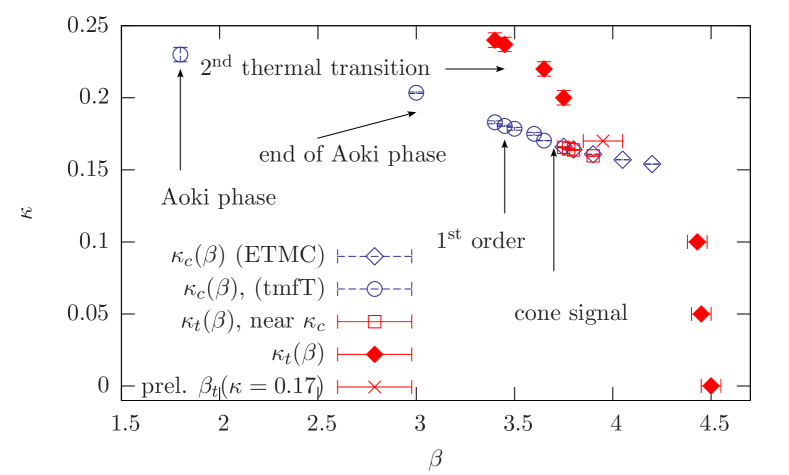
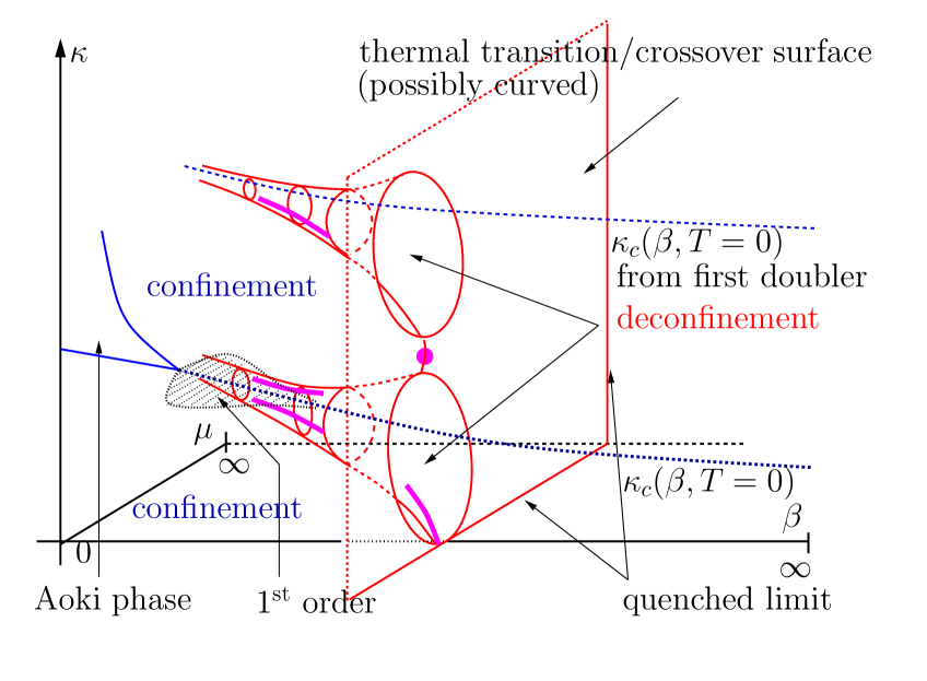
Figure 1: Left: Map of our simulations performed at $\mu<0.007$. Right: Emerging phase structure; regions identified by tmfT measurements are marked by magenta symbols.

3 Simulation results

The simulations were mainly performed on lattices of spatial size $N_{\sigma}=16$ and $N_{\tau}=8$. The algorithm in use is described in Ref. [17]. An overview of the regions covered by our simulation is presented in the left panel of Fig. 1. It contains all transition and crossover points that we found in our simulations and is supplemented by data describing the $T=0$ critical line $\kappa_{c}(\beta\geq 3.75)$ provided by the ETM collaboration.

After the unsuccessful search reported in [7], we have checked the existence of the Aoki phase at the three values $\beta\>\in\>\{1.8,\,3.0,\,3.4\}$. The necessary and sufficient condition for spontaneous symmetry breaking reads

$$\lim\limits_{h\to 0}\lim\limits_{N_{\sigma}\to\infty}\langle\bar{\psi}i\gamma_{5}\tau^{3}\psi\rangle_{N_{\sigma},\,h}\neq 0\,.$$ (1)

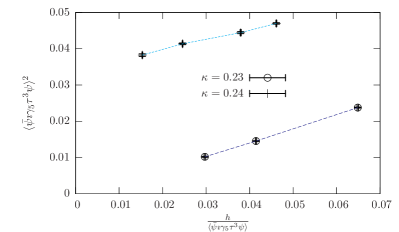
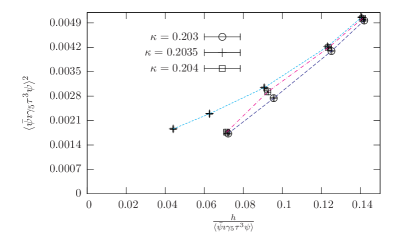
Figure 2: Fisher plots for the order parameter $\langle\bar{\psi}i\gamma_{5}\tau^{3}\psi\rangle$ describing its limit for $h=2\kappa\mu\to 0$; left: $\beta=1.8$, right: $\beta=3.0$ .

Figure 2 shows the Fisher plots [13] of the order parameter $\langle\bar{\psi}i\gamma_{5}\tau^{3}\psi\rangle$ as a function of $h/\langle\bar{\psi}i\gamma_{5}\tau^{3}\psi\rangle$, with $h=2\kappa\mu$, for $\beta=1.8$ and $3.0$. The condensate has a finite limit for $h\to 0$ (a positive intercept at $h=0$) for suitable $\kappa$ values. For the smallest value $\beta=1.8$, the left panel of Fig. 2 gives convincing evidence for the onset of spontaneous symmetry breaking somewhere in the range $0.24>\kappa>0.23$. The right panel strongly indicates that at $\beta=3.0$ the symmetry-broken phase – if it exists at all – is realized only in the interval $0.203<\kappa<0.204$. A volume extrapolation would be welcome but is unavailable at this $\beta-$value. This marks the lower boundary $\kappa_{c}^{\rm lower}(\beta)$ of the Aoki phase. We have not systematically searched for its upper boundary $\kappa_{c}^{\rm upper}(\beta)$.

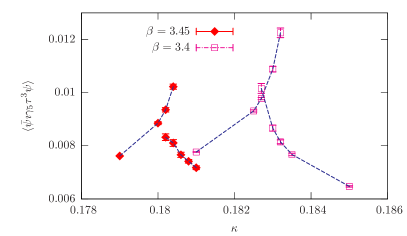
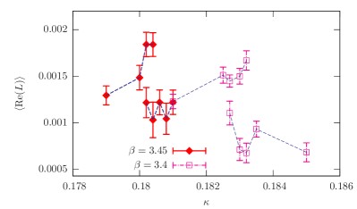
Figure 3: Signals of metastability at $\beta=3.4$ and 3.45. The two-state signal left: in the pseudoscalar condensate, right: in the real part of the Polyakov loop.

At $\beta=3.4$ we reinforce our preliminary results published in Ref. [7] that, instead of an Aoki phase, there are strong metastabilities when simulating at finite twist $\mu\approx 0.0068$. This confirms the first-order Sharpe-Singleton scenario, and represents a remnant of the phase structure at $T=0$ (on symmetric lattices). This is shown for $\beta=3.4$ and $3.45$ in Fig. 3 for the order parameter (left) and the Polyakov loop (right). The behaviour of the latter at this transition cannot be interpreted as thermal. Also the average plaquette (as checked at $\beta=3.4$ and $\kappa=0.1827$) is running in separate, metastable histories starting from hotter/colder neighbouring states.

In the range $3.4\leq\beta\leq 3.65$ between strong and weak coupling, simulating at $\mu=0.0068$, we see a finite temperature transition, located at $\kappa_{T}\gg\kappa_{c}(\beta)$, i.e. far above the chiral line for $T=0$. The transition is inherited from the first doubler structure existing at higher $\kappa$. The corresponding $\kappa_{T}(\beta,\mu)$ evolves rapidly with $\beta$, moving closer towards the critical line $\kappa_{c}(\beta)$ with increasing $\beta$ (cf. Fig. 1). The transition is possibly of first order as indicated by histograms of the Polyakov loop at $\beta=3.6$ in the interval $0.18<\kappa<0.24$: they show a relatively flat but clear double peak structure at $\kappa=0.22$. On $32^{3}\times 8$ lattices simulated at the same $\beta-\kappa-\mu-$point one observes long-living metastability in the Polyakov loop. Also at higher $\beta=3.75$ this thermal transition continues to exist, still separated from the unfolding thermal transition surface around $\kappa_{c}(\beta)$. Finally, it appears to join the latter in the neighbourhood of $\beta=4.0$. Before this joining happens, Fig. 4 shows the characteristic behaviour of the Polyakov loop and its susceptibility measured at $\beta=3.75$ with $\mu=0.005$ over an interval $0.16<\kappa\leq 0.21$ that is covering both transition regions. The two peaks are clearly visible, but the lower susceptibility peak is not yet well resolved on the coarse $\kappa$ scale of Fig. 4.

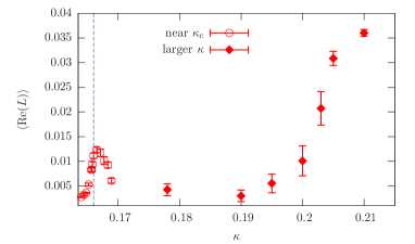
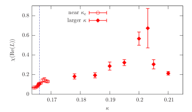
Figure 4: Left: real part of the Polyakov loop, right: its susceptibility as functions of $\kappa$ for $\beta=3.75$ and $\mu=0.005$. The dashed line marks $\kappa_{c}(\beta=3.75,T=0)$.

It is our goal to work at maximal twist, thus ultimately we need to resolve the lower peak in Fig. 4. The position and nature of the first (i.e. lower in $\kappa$) finite temperature transition/crossover, when studied at $\mu\neq 0$, changes considerably between the metastability region described by Fig. 3 and the scaling region. Midway between the two, at $\beta=3.65$, one sees the Polyakov loop entering and then leaving again a narrow deconfining region in $\kappa$ (cf. the left panel of Fig. 5). Approaching the physically relevant scaling region, $\beta\gtrsim 3.75$, the peak structure grows even clearer. The narrow peak (supposed to contain the deconfined phase) moves gradually further to lower $\kappa$ with rising $\beta=3.75$, $3.775$ and $\beta=3.8$ (cf. the right panel of Fig. 5).

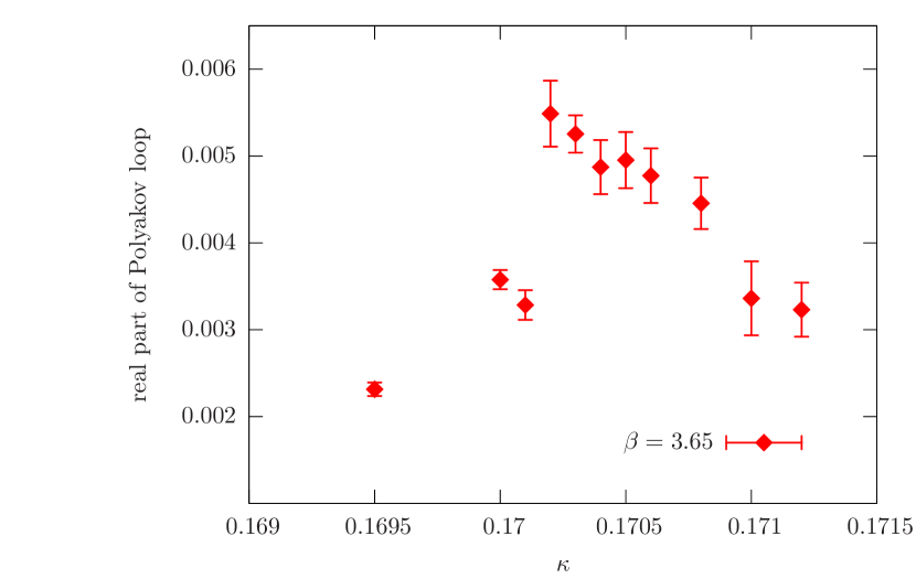
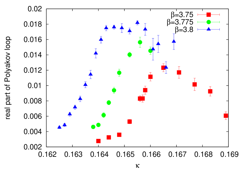
Figure 5: The real part of the Polyakov loop as function of $\kappa$; left: for $\beta=3.65$ with $\mu=0.0068$, right: for $\beta=3.75$, $3.775$ and $3.8$ (all with $\mu=0.005$).

With a large computational effort the rise and decline of the Polyakov loop begins to be reflected also in the corresponding susceptibility. The Polyakov loop susceptibility gradually develops a double peak which is already clearly visible at $\beta=3.8$ (cf. the left panel of Fig. 6). Remarkably, the lower$-\kappa$ peak is accompanied by a peak of the pion norm (presented in the right panel of Fig. 6) emphasizing the entrance into the deconfining and chiral-symmetry restored phase. So far, within the presently available statistics, we could not detect a significant similar chiral signal marking the exit.

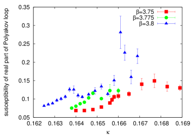
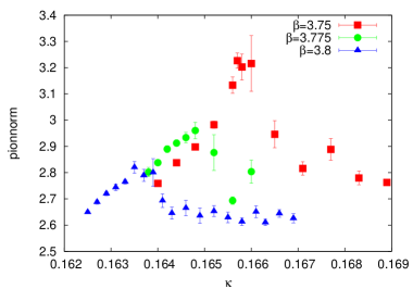
Figure 6: Left: the susceptibility of the Polyakov loop, right: the pion norm as functions of $\kappa$ for $\beta=3.75$, $3.775$ and $3.8$ (all at $\mu=0.005$).

4 The cone signal and comparison with lattice $\chi{\rm PT}$

We interpret the structured signal in the Polyakov loop near $\kappa_{c}$ outlined in the preceding section as a numerical indication for passing through a confinement$\rightarrow$deconfinement crossover approaching $\kappa_{c}$ from small positive quark mass, followed by a deconfinement$\rightarrow$confinement crossover at small negative quark mass. This picture is qualitatively consistent with the conical structure predicted by Creutz (see also Fig. 1). The thermal transition takes place at a given value of the quark mass which is determined by the parameters $\kappa$ and $\mu$. At tree level the according relation reads:

$$m_{q}^{2}=\mu^{2}+\frac{1}{4}\left(\frac{1}{\kappa}-\frac{1}{\kappa_{c}}\right)^{2}\,.$$ (2)

Using lattice chiral perturbation theory (L$\chi{\rm PT}$), one obtains the following modification of (2) in NLO (cf. [18]):

$$m_{q}^{2}=\left(\frac{1}{Z_{P}^{2}}\mu^{2}+\frac{1}{Z_{S}^{2}}\frac{1}{4}\left(\frac{1}{\kappa}-\frac{1}{\kappa_{c}}\right)^{2}\right)\left(1+K\cos\omega\right)^{2}\,.$$ (3)

From the zero temperature simulations of the ETM collaboration we know that $\kappa_{c}(\beta=3.75)=0.1660(1)$, $Z_{S}\approx 0.6$ and $Z_{P}\approx 0.3$. $K$ is an unknown $O(a)$ coefficient that is introduced by L$\chi{\rm PT}$. The twist angle $\omega$ is defined by $\tan\omega=\mu/\left(0.5\left(1/\kappa-1/\kappa_{c}\right)\right)$.

In Fig. 7 the thermal transition points that we have found at $\beta=3.75$ for $\mu=0.005$ and $0.007$ are compared with the two relations above. In principle, $K$ and $m_{q}$ can be determined from a fit. However, given the rather large uncertainties of $Z_{P}$ and $Z_{S}$ and also the small number of available data points, we are only able to check whether the formulae are capable of describing the data. For the tree level formula this is not the case (in the plot: $m_{q}=0.01$, $\kappa_{c}=0.1660$), due to the $\kappa\leftrightarrow\left(2/\kappa_{c}-1/\kappa\right)$-symmetry of equation (2). However, choosing $m_{q}=0.028$, $K=0.5$, $Z_{S}=0.6$, $Z_{P}=0.3$ and $\kappa_{c}=0.1660$ the NLO formula (3) is consistent with the data points.

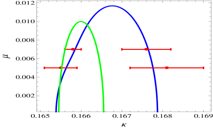
Figure 7: Thermal transition points found at $\beta=3.75$ with $\kappa_{c}=0.1660$ compared to tree level ($m_{q}=0.01$, green) and L$\chi{\rm PT}$ ($m_{q}=0.028$, $K=0.5$, $Z_{S}=0.6$, $Z_{P}=0.3$, blue) curves.

5 Summary and outlook

We investigated the global phase structure of 2-flavour Wilson-twisted-mass LQCD with a tree-level Symanzik-improved gauge action. Our simulation results support the existence of an Aoki phase (at $\beta\lesssim 3.0$) as well as the first-order Sharpe-Singleton-scenario at finite twist (for $\beta\approx 3.4$). Moreover, we find indications of a conical structure of the finite-temperature crossover surface in a bounded $\beta-$interval, $3.65\leq\beta\leq 3.8$, with $\mu=0.005$ and $0.007$. Our next steps will be the localization of additional finite temperature crossover points to refine the L$\chi{\rm PT}-$prediction of the transition line and to bound the value $\mu_{T}$ for the thermal crossover at maximal twist within a narrow interval. Depending on the findings of this investigation, a subsequent simulation at maximal twist to detect $\mu_{T}$ numerically will follow.

Acknowledgements. It is a pleasure to thank Steve Sharpe, André Sternbeck and Carsten Urbach for discussions. In addition, we thank André for joining our phone conferences and Carsten for supplying the HMC code. Most simulations have been done at the apeNEXT in Rome and DESY-Zeuthen. This work has been supported in part by the DFG Sonderforschungsbereich/Transregio SFB/TR9-03. O. P. and L. Z. acknowledge support by the DFG project PH 158/3-1. E.-M. I. was supported by DFG under contract FOR 465 / Mu932/2 (Forschergruppe Gitter-Hadronen-Phänomenologie). He is grateful to the Karl-Franzens-Universität Graz for the guest position he holds while this paper is written up.

References

- [1] E.-M. Ilgenfritz et al., \posPoS(LAT2006)140, [arXiv:hep-lat/0610112].
- [2] A. Shindler, Phys. Rept. 461 (2008) 37, [arXiv:0707.4093[hep-lat]]
- [3] K. Jansen, plenary talk at this conference.
- [4] M. Creutz, \posPoS(LAT2007)007, [arXiv:0708.1295[hep-lat]].
- [5] Ph. Boucaud et al. (ETM collaboration), [arXiv:0803.0224[hep-lat]].
- [6] Ph. Boucaud et al. (ETM collaboration), Phys. Lett. B650 (2007) 304, [arXiv:hep-lat/0701012].
- [7] E.-M. Ilgenfritz et al., \posPoS(LAT2007)238, [arXiv:0710.0569[hep-lat]].
- [8] M. Creutz, Phys. Rev. D76 (2007) 054501, [arXiv:0706.1207[hep-lat]].
- [9] M. Creutz, [arXiv:hep-lat/9608024].
- [10] S. R. Sharpe and J. M. S. Wu, Phys. Rev. D70 (2004) 094029, [arXiv:hep-lat/0407025].
- [11] G. Münster, JHEP 09 (2004) 035, [arXiv:hep-lat/0407006].
- [12] F. Farchioni et. al., Eur. Phys. J. C39 (2005) 421, [arXiv:hep-lat/0406039].
- [13] E.-M. Ilgenfritz et al., Phys. Rev. D 69 (2004) 074511, [arXiv:hep-lat/0309057].
- [14] F. Farchioni et. al., Eur. Phys. J. C42 (2005) 73, [arXiv:hep-lat/0410031].
- [15] N. Ukita et al., \posPoS(LAT2006)150, [arXiv:hep-lat/0610038].
- [16] V. G. Bornyakov, et al. (DIK collaboration), \posPoS(LAT2007)171, [arXiv:0711.1427[hep-lat]].
- [17] C. Urbach et al., Comput. Phys. Commun. 174 (2006) 87, [arXiv:hep-lat/0506011].
- [18] S. R. Sharpe, [arXiv:hep-lat/0607016].