Bayesian detection of unmodeled bursts of gravitational waves.

Abstract

The data analysis problem of coherently searching for unmodeled gravitational-wave bursts in the data generated by a global network of gravitational-wave observatories has been at the center of research for almost two decades. As data from these detectors is starting to be analyzed, a renewed interest in this problem has been sparked. A Bayesian approach to the problem of coherently searching for gravitational wave bursts with a network of ground-based interferometers is here presented. We demonstrate how to systematically incorporate prior information on the burst signal and its source into the analysis. This information may range from the very minimal, such as best-guess durations, bandwidths, or polarization content, to complete prior knowledge of the signal waveforms and the distribution of sources through spacetime. We show that this comprehensive Bayesian formulation contains several previously proposed detection statistics as special limiting cases, and demonstrate that it outperforms them.

1 Introduction

Large-scale, broad-band interferometric gravitational-wave observatories [1, 2, 3, 4] are operating at their anticipated sensitivities, and scientists around the globe have begun to analyze the data generated by these instruments in search of gravitational wave signals [5]. Gravitational wave bursts (GWBs) are among the most exciting signals scientists expect to observe, as our present knowledge and modeling ability of GWB-emitting systems is rather limited. These signals often depend on complicated (and interesting) physics, such as dynamical gravity and the equation of state of matter at nuclear densities. While this makes GWBs an especially attractive target to study, our lack of knowledge also limits the sensitivity of searches for GWBs. Potential sources of GWBs include merging compact objects [6, 7, 8, 9, 10, 11, 12, 13, 14], core-collapse supernovae [15, 16, 17, 18, 19], and gamma-ray burst engines [20]; see [21] for an overview.

Although a gravitational wave signal is characterized by two independent polarizations, an interferometric gravitational wave detector is sensitive to a single linear combination of them. Simultaneous observations of a gravitational wave burst by three or more observatories over-determines the waveform, permitting the source position on the sky to be determined, and a least-squares estimate of the two polarizations. This solution of the inverse problem for gravitational waves was first derived by Gürsel and Tinto [22] for three interferometers. Subsequent work generalized it [23] and formalized it as an example of a coherent maximum likelihood statistic by Flanagan and Hughes [7] and later Anderson, Brady, Creighton, and Flanagan [24]. Various modifications have been proposed, such as Rakhmanov’s Tikhonov [25] and Summerscale’s maximum-entropy [26] regularization techniques, Kilmenko et al’s constraint likelihood method [27, 28], and the SNR variability approach of Mohanty et al. [28]. Potential as a consistency test was noted by Wen and Schutz in [29] and demonstrated in Chatterji et al [30]. Other coherent detection algorithms have been proposed by Sylvestre [31] and by Arnaud et al. [32].

These approaches to signal detection have generally been derived by following either ad hoc reasoning or a maximum-likelihood criterion (notable exceptions, foreshadowing our Bayesian approach, are Finn [33], Anderson et al [24] and Allen et al [34]). In this paper we present a systematic and comprehensive Bayesian formulation [35, 36] of the problem of coherent detection of gravitational wave bursts. We demonstrate how to incorporate partial or incomplete knowledge of the signal in the analysis, thereby improve the probability of detection of these weak signals. This information may include time-frequency properties of the signal, polarization content, model waveform families or templates, as well as information on the distribution of the source through spacetime. We also explicitly identify the prior assumptions that must be made about the signal to cause a Bayesian analysis to behave like several of the previously proposed detection statistics.

Real interferometers also experience instrumental artifacts that can masquerade as signals. These are typically dealt with in post-processing rather than by the detection statistic itself, but some proposals have been made to include a model for these “glitches” in the detection statistic [37, 38]. An advantage of the Bayesian framework is that the standard choice between signal and stationary noise could be extended to include a third option: randomly occurring noise “glitches”. This formulation is a promising direction for future progress, but we do not further discuss it in this paper.

The paper is organized as follows. In §2 we derive the Bayesian posterior detection probability of an idealized delta-like burst signal by a toy-model network of observatories. Greatly expanding on [38], we then generalize the derivation of the Bayesian odds ratio into a usable statistic for an arbitrary number of interferometers with differently colored and (potentially) correlated noises. We also consider a wide range of signal models corresponding to different states of knowledge about the burst, from total ignorance to complete a priori knowledge of the waveforms. In §3 we characterize the relative performance of previously proposed statistics (the Gürsel-Tinto/standard and constraint likelihoods) and the Bayesian statistic by performing a Monte-Carlo simulation in which we add a simple binary black-hole merger waveform to simulated detector data and construct Receiver-Operating Characteristic (ROC) curves. We find that the Bayesian method increases the probability of detection for a given false alarm rate by approximately 50%, over those associated with previously proposed statistics.

2 Analysis

2.1 Single-sample observation

We begin by investigating perhaps the simplest Bayesian coherent data analysis: detecting a signal from a known sky position in a single strain sample from each of $N$ gravitational wave observatories. This example will show many of the basic features of the Bayesian analysis, and highlight some of the differences between the Bayesian approach and previous statistics. In the following section we will generalize to a multi-sample search for a signal arriving at an unknown time from an unknown sky position.

Consider a single strain sample from each of $N$ detectors, each measurement taken at the moment corresponding to the passage of a postulated plane gravitational wave from some known location on the sky, ($\theta,\phi$). The measurements are then equal to [22]

$$\mathbf{x}=\mathbf{F}\,\mathbf{h}+\mathbf{e}\,,$$ (1)

where $\mathbf{x}$ is the vector of measurements $[x_{1},\ldots,x_{N}]^{T}$, the matrix $\mathbf{F}=[[F_{1}^{+},F_{1}^{\times}],\ldots,[F_{N}^{+},F_{N}^{\times}]]$ contains the antenna responses of the observatories to the postulated gravitational wave strain vector $\mathbf{h}=[h_{+},h_{\times}]^{T}$, and $\mathbf{e}$ is the noise in each sample. $\mathbf{F}$ is a known function of the source sky direction $(\theta,\phi)$, and the decomposition into $+$ and $\times$ polarizations requires us to choose an arbitrary polarization basis angle $\psi$ for each source sky direction.

We wish to distinguish between two hypotheses: $H_{0}$, that the data contains only noise, and $H_{1}$, that the data contains a gravitational wave signal. The Bayesian odds ratio [35, 36] allows us to compare the plausibility of the hypotheses:

$$\frac{p(H_{1}|\mathbf{x},I)}{p(H_{0}|\mathbf{x},I)}=\frac{p(H_{1}|I)}{p(H_{0}|I)}\frac{p(\mathbf{x}|H_{1},I)}{p(\mathbf{x}|H_{0},I)}\,,$$ (2)

where $I$ is a set of unstated but shared assumptions (such as the detector locations, orientations and noise power spectra). If the posterior plausibility ratio is greater than one, $H_{1}$ is more plausible than $H_{0}$ and we classify the observation as a detection. If the posterior plausibility ratio is less than one, $H_{1}$ is less plausible than $H_{0}$ and we classify the observation as a non-detection.

The $p(H|I)$ terms (“plausibility of $H$ assuming $I$”)are the prior plausibilities we assign to each hypothesis $H$ on the basis of our knowledge $I$ prior to considering the measurement; for example, our expectation that detectable gravitational waves are rare requires that $p(H_{1}|I)\ll p(H_{0}|I)$.

The $p(\mathbf{x}|H,I)$ terms (“plausibility of $\mathbf{x}$ assuming $H$ and $I$”) are the probabilities assigned by a hypothesis to the occurrence of a particular observation $\mathbf{x}$. These are sometimes called likelihood functions; they represent the likelihood of a certain measurement being made.

The $p(H|\textbf{x},I)$ terms are the posterior plausibilities we assign to the hypotheses in light of the observation. The hypothesis that assigned more probability to the observation becomes more plausible.

For notational simplicity we will drop the $I$ in our formulae; the unstated assumptions are implicit.

If we make the idealized assumption that the noise in each detector is independent and normally distributed [35, 36] with zero mean and unit standard deviation, we can then write the following expression for the likelihood $p(\mathbf{x}|H_{0})$

$$p(\mathbf{x}|H_{0}) = \prod_{i=1}^{N}p(x_{i}|H_{0})$$ (3)

$$= \prod_{i=1}^{N}\frac{1}{\sqrt{2\pi}}\exp(-\frac{1}{2}x_{i}^{2})$$

$$= (2\pi)^{-\frac{N}{2}}\exp(-\frac{1}{2}\mathbf{x}^{T}\mathbf{x})\,,$$

where ^T denotes matrix transposition. For real detectors, the measurements can be whitened, which modifies the effective beam pattern functions $\mathbf{F}$.

If we assume that there is a gravitational wave $\mathbf{h}$ present, then after subtracting away the response $\mathbf{F}\,\mathbf{h}$ the data will be distributed as noise and the likelihood $p(\mathbf{x}|\mathbf{h},H_{1})$ becomes

$$p(\mathbf{x}|\mathbf{h},H_{1}) = (2\pi)^{-\frac{N}{2}}\exp(-\frac{1}{2}(\mathbf{x}-\mathbf{F}\,\mathbf{h})^{T}(\mathbf{x}-\mathbf{F}\,\mathbf{h}))\,.$$ (4)

Unfortunately, we do not know the signal strain vector $\mathbf{h}$ a priori. To compute the plausibility of the more general hypothesis $p(\mathbf{x}|H_{\mathrm{signal}})$ we need to marginalize away these nuisance parameters

$$p(\mathbf{x}|H_{1}) = \int_{-\infty}^{+\infty}\int_{-\infty}^{+\infty}p(\mathbf{h}|H_{1})p(\mathbf{x}|\mathbf{h},H_{1})\,\mathrm{d}{h_{+}}\,\mathrm{d}{h_{\times}}\,.$$ (5)

The hypothesis resulting from the marginalization integral is an average of the hypotheses for particular signals $\mathbf{h}$, weighted by the prior probability $p(\mathbf{h}|H_{\mathrm{signal}})$ we assign to those signals occurring. A convenient choice of prior is to use a normal distribution for each polarization, with a standard deviation $\sigma$ indicative of the amplitude scale of gravitational waves we hope to detect. Under these assumptions the prior is

$$p(\mathbf{h}|H_{1}) = \frac{1}{2\pi\sigma^{2}}\exp(-\frac{1}{2\sigma^{2}}\mathbf{h}^{T}\mathbf{h})\,.$$ (6)

This allows us to perform the marginalization integral analytically

$$p(\mathbf{x}|H_{1}) = (2\pi)^{-\frac{N}{2}-1}\sigma^{-2}\int_{-\infty}^{+\infty}\int_{-\infty}^{+\infty}\exp(-\frac{1}{2}((\mathbf{x}-\mathbf{F}\,\mathbf{h})^{T}(\mathbf{x}-\mathbf{F}\,\mathbf{h})$$ (7)

$$\mbox{}+\sigma^{-2}\mathbf{h}^{T}\mathbf{h}))\,\mathrm{d}{h_{+}}\,\mathrm{d}{h_{\times}}$$

$$= (2\pi)^{-\frac{N}{2}}|\mathbf{I-K_{\mathrm{ss}}}|^{\frac{1}{2}}\exp(-\frac{1}{2}\,\mathbf{x}^{T}(\mathbf{I-K_{\mathrm{ss}}})\mathbf{x})\,,$$

where

$$\mathbf{K_{\mathrm{ss}}} \equiv \mathbf{F}(\mathbf{F}^{T}\mathbf{F}+\sigma^{-2}\mathbf{I})^{-1}\mathbf{F}^{T}.$$ (8)

The result is a multivariate normal distribution with covariance matrix $(\mathbf{I-K_{\mathrm{ss}}})^{-1}$, which quantifies the correlations among the detectors due to the presence of a gravitational wave signal.

With both hypotheses defined, we can form the likelihood ratio

$$\Lambda = \frac{p(\mathbf{x}|H_{1})}{p(\mathbf{x}|H_{0})}$$ (9)

$$= |\mathbf{I-K_{\mathrm{ss}}}|^{\frac{1}{2}}\exp(\frac{1}{2}\,\mathbf{x}^{T}\mathbf{F}(\mathbf{F}^{T}\mathbf{F}+\sigma^{-2}\mathbf{I})^{-1}\mathbf{F}^{T}\mathbf{x})\,.\,$$

Multiplying the likelihood ratio by the prior plausibility ratio $p(H_{1})/p(H_{0})$ completes the calculation of the Bayesian odds ratio (2).

In the limit $\sigma\rightarrow\infty$ we find that the odds ratio contains the least-squares estimate of the strain

$$\mathbf{\hat{h}} = (\mathbf{F}^{T}\mathbf{F})^{-1}\mathbf{F}^{T}\mathbf{x}\,.$$ (10)

The odds ratio may then be rewritten in terms of a matched filter for the response to the estimated strain, $\mathbf{x}^{T}\mathbf{F}\,\mathbf{\hat{h}}$. For finite values of $\sigma$, the odds ratio contains the Tikhonov regularized estimate of the strain [25]

$$\mathbf{\hat{h}}=(\mathbf{F}^{T}\mathbf{F}+\sigma^{-2}\mathbf{I})^{-1}\mathbf{F}^{T}\mathbf{x}\,,$$ (11)

and can still be rewritten as a matched filter for this estimate.

It is also worth noting the presence in (9) of the determinant $|\mathbf{I-K_{\mathrm{ss}}}|$ factor. It is independent of the data and depends only on the antenna pattern and the signal model. In particular, it tells us how strongly to weight likelihoods computed for different possible sky positions of the signal. This Occam factor penalizes sky positions of high sensitivity relative to sky positions of lower sensitivity which give similar exponential part of the likelihood. The effect is typically small compared to the exponential in most cases if the data has good evidence for a signal, but can be important for weak signals and for parameter estimation.

2.2 General Bayesian model

We now generalize the analysis of the previous section to the case of burst signals of extended duration and unknown source sky direction $(\theta,\phi)$ and arrival time $\tau$ with respect to the centre of the Earth.

A global network of $N$ gravitational wave detectors each produce a time-series of $M$ observations with sampling frequency $f_{\textrm{s}}$, which we pack into a single vector

$$\mathbf{x}=[x_{1,1},x_{1,2},\ldots,x_{1,M},x_{2,1},x_{2,2},\ldots,x_{2,M},\ldots,x_{N,1},x_{N,2},\ldots,x_{N,M}]^{T}\ .$$ (12)

Our signal model is a generalization of (1),

$$\mathbf{x} = \mathbf{F}(\tau,\theta,\phi)\cdot\mathbf{h}+\mathbf{e}\,,$$ (13)

where

$$\mathbf{h} = [h_{+,1},h_{+,2},\ldots,h_{+,L},h_{\times,1},\ldots,h_{\times,L}]^{T}$$ (14)

is a time-series of $2L$ samples describing the band-limited strain waveform (with the two polarizations packed into a single vector), $\mathbf{e}$ is a random variable representing the instrumental noise, and $\mathbf{F}(\tau,\theta,\phi)$ is a $NM\times 2L$ response matrix describing the response of each observatory to an incoming gravitational wave,

$$\mathbf{F}(\tau,\theta,\phi) = \left[\begin{array}[]{cc}F^{+}_{1}(\theta,\phi)\mathbf{T}(\tau+\Delta\tau_{1}(\theta,\phi))&F^{\times}_{1}(\theta,\phi)\mathbf{T}(\tau+\Delta\tau_{1}(\theta,\phi))\\ F^{+}_{2}(\theta,\phi)\mathbf{T}(\tau+\Delta\tau_{2}(\theta,\phi))&F^{\times}_{2}(\theta,\phi)\mathbf{T}(\tau+\Delta\tau_{2}(\theta,\phi))\\ \vdots&\vdots\\ F^{+}_{N}(\theta,\phi)\mathbf{T}(\tau+\Delta\tau_{N}(\theta,\phi))&F^{\times}_{N}(\theta,\phi)\mathbf{T}(\tau+\Delta\tau_{N}(\theta,\phi))\end{array}\right]\,.$$ (19)

Each $M\times L$ block of the response matrix is responsible for scaling and time shifting one of the waveform polarizations for one detector, so each block is the product of the directional sensitivity of each detector to each polarization, $F^{+}_{i}(\theta,\phi)$ or $F^{\times}_{i}(\theta,\phi)$, and a time delay matrix $T_{j,k}(t)$ , for the source sky direction dependent arrival times $\tau+\Delta\tau_{i}(\theta,\phi)$ at each detector.

2.3 Noise model

The noise that affects gravitational wave detectors is typically modeled as stationary, colored gaussian noise that is independent of the signal parameters. This can be represented with a multivariate normal distribution, which can be compactly written as

$$\mathcal{N}(\mathbf{\mu},\mathbf{\Sigma},\mathbf{x}) = \frac{1}{(2\pi)^{N/2}\sqrt{|\mathbf{\Sigma}|}}\exp(-\frac{1}{2}(\mathbf{x}-\mathbf{\mu})^{T}\mathbf{\Sigma}^{-1}(\mathbf{x}-\mathbf{\mu}))\,.$$ (20)

The vector $\mathbf{\mu}$ is the mean of the distribution, and the positive-definite covariance matrix $\mathbf{\Sigma}$ describes the ellipsoidal shape of the constant-density contours of the distribution in terms of the pairwise covariances of the samples,

$$\mathbf{\Sigma}_{i,j}=\langle(e_{i}-\mu_{i}),(e_{j}-\mu_{j})\rangle\,.$$ (21)

Using this notation, the noise likelihood is

$$p(\mathbf{x}|H_{0}) = \mathcal{N}(\mathbf{0},\mathbf{\Sigma},\mathbf{e})$$ (22)

for some $MN\times MN$ positive definite matrix $\mathbf{\Sigma}$. Under the additional assumption of stationarity over some timescale, these covariances can be estimated from previous observations.

In the case of Gaussian stationary colored noise, each detector is individually represented by a Toeplitz covariance matrix $\mathbf{\Sigma}^{(i)}$. For uncorrelated noise, the covariance matrix for the whole network is $\mathbf{\Sigma}=\textrm{diag}(\mathbf{\Sigma}^{(1)},\mathbf{\Sigma}^{(2)},\ldots,\mathbf{\Sigma}^{(N)})$. In the simple case in which all the noises are white, have equal standard deviation and are uncorrelated, we have $\mathbf{\Sigma}=\textrm{diag}(\mathbf{I},\mathbf{I},\ldots,\mathbf{I})=\mathbf{I}$.

The generalization of (4) and (5) for the signal likelihood is

$$p(\mathbf{x}|H_{1}) = \int_{V_{\mathbf{h},\tau,\theta,\phi}}\!\!\!\!\!\!\!\!\!\mathcal{N}(\mathbf{F}(\tau,\theta,\phi)\cdot\mathbf{h},\mathbf{\Sigma},\mathbf{x})\,p(\mathbf{h},\tau,\theta,\phi|H_{1})\,\mathrm{d}\mathbf{h}\ldots\mathrm{d}\phi\ ,$$ (23)

where ${V_{\mathbf{h},\tau,\theta,\phi}}$ is the space of all signal parameters and $p(\mathbf{h},\tau,\theta,\phi|H_{1})$ is the prior for these parameters. Without loss of generality we may separate this signal prior into a prior on source sky direction and arrival time, and a prior on the waveform conditional on the source sky direction and the arrival time, i.e.

$$p(\mathbf{h},\tau,\theta,\phi|H_{1})=p(\tau,\theta,\phi|H_{1})\,p(\mathbf{h}|\tau,\theta,\phi,H_{1})\,,$$ (24)

giving

$$p(\mathbf{x}|H_{1}) = \int_{V_{\mathbf{h},\tau,\theta,\phi}}\!\!\!\!\!\!\!\!\!\mathcal{N}(\mathbf{F}(\tau,\theta,\phi)\cdot\mathbf{h},\mathbf{\Sigma},\mathbf{x})\,p(\tau,\theta,\phi|H_{1})\,p(\mathbf{h}|\tau,\theta,\phi,H_{1})\,\mathrm{d}\mathbf{h}\ldots\mathrm{d}\phi\ .$$ (25)

2.4 Wideband signal model

In analogy with the single sample case, we can choose a multivariate normal distribution prior for the waveform amplitudes and render the integral soluble in closed form. The marginalization integral over $\mathbf{h}$ in (25) can then be analytically performed, giving

$$\frac{p(\mathbf{x}|\tau,\theta,\phi,H_{1})}{p(\mathbf{x}|H_{0})} = \frac{\int_{\mathbb{R}^{2L}}\mathcal{N}(\mathbf{F}(\tau,\theta,\phi)\cdot\mathbf{h},\mathbf{\Sigma},\mathbf{x})\,p(\mathbf{h}|\tau,\theta,\phi,H_{1})\,\mathrm{d}\mathbf{h}}{\mathcal{N}(\mathbf{0},\mathbf{\Sigma},\mathbf{x})}$$ (26)

(see (34) below). Numerical integration over a more manageable three dimensions is then sufficient to compute the Bayes factor,

$$\frac{p(\mathbf{x}|H_{1})}{p(\mathbf{x}|H_{0})} = \int\int\int p(\tau,\theta,\phi|H_{1})\,\frac{p(\mathbf{x}|\tau,\theta,\phi,H_{1})}{p(\mathbf{x}|H_{0})}\,\mathrm{d}\tau\,\mathrm{d}\theta\,\mathrm{d}\phi\,.$$ (27)

This signal model is computationally tractable. It represents signals that can be described by an invertible $2L\times 2L$ correlation matrix, including the important ’least informative’ case of independent, normally distributed samples of $\mathbf{h}$.

2.5 Informative signal models

The wideband signal model excludes some important cases, such as when we have a known waveform, almost known waveform (such as from a family of numerical simulations) or even just a signal restricted to some frequency-band. These signals are superpositions of a (relatively) small number $G<2L$ of basis waveforms, that may themselves be characterized by a finite number of parameters, which we denote $\rho$. These parameters must be numerically integrated, like $\tau$, $\theta$, and $\phi$, which may be time-consuming. Their prior distribution will be denoted by $p(\mathbf{\rho}|\tau,\theta,\phi,H_{1})$.

To describe the signal as a superposition of basis waveforms [39], define a set of amplitude parameters $\mathbf{a}$ mapped into strain $\mathbf{h}$ via a $2L\times G$ matrix $\mathbf{W}(\rho,\tau,\theta,\phi)$ whose columns $\mathbf{w}_{i}(\rho,\tau,\theta,\phi)$ are the basis waveforms, so that

$$\mathbf{h} = \mathbf{W}(\mathbf{\rho},\tau,\theta,\phi)\cdot\mathbf{a}\ .$$ (28)

We assume that the amplitude parameters $\mathbf{a}$ are multivariate normal distributed with a covariance matrix $\mathbf{A}(\mathbf{\rho},\tau,\theta,\phi)$, so that

$$p(\mathbf{a}|\mathbf{\rho},\tau,\theta,\phi,H_{1}) = \mathcal{N}(\mathbf{0},\mathbf{A}(\mathbf{\rho},\tau,\theta,\phi),\mathbf{a})\,.$$ (29)

The resulting distribution for the waveform strain is

$$p(\mathbf{h}|\tau,\theta,\phi,H_{1}) = \int_{V_{\rho}}\int_{\mathbb{R}^{G}}p(\mathbf{h}|\mathbf{a},\mathbf{\rho},\tau,\theta,\phi,H_{1})\,p(\mathbf{a},\mathbf{\rho}|\tau,\theta,\phi,H_{1})\,\mathrm{d}\mathbf{a}\,\mathrm{d}\mathbf{\rho}\,$$ (30)

$$= \int_{V_{\rho}}\int_{\mathbb{R}^{G}}\delta(\mathbf{h}-\mathbf{W}\cdot\mathbf{a})\,\mathcal{N}(\mathbf{0},\mathbf{A},\mathbf{a})\,p(\mathbf{\rho}|\tau,\theta,\phi,H_{1})\,\mathrm{d}\mathbf{a}\,\mathrm{d}\mathbf{\rho}\,,$$

where for clarity we have begun to omit the dependence of matrices on their parameters. As $G<2L$ (i.e., we have fewer basis waveforms than samples in the signal time-series) the integral over $\mathbf{a}$ cannot be directly represented as a multivariate normal distribution.

This signal model proposes that gravitational wave signals have waveforms that are the sum of $G$ basis waveforms with amplitudes that are normally distributed (and potentially correlated). The basis waveforms and their amplitude distributions may vary with source sky direction, arrival time, and any other parameters we care to include in $\mathbf{\rho}$. The model is capable of representing a variety of sources including the important special cases of known ‘template’ waveforms, and band-limited bursts. We will consider some concrete examples in §2.6; perhaps the most important is a scale parameter $\sigma$, that permits us to look for signals of different total energies.

We can substitute the expression back into part of (26) to form a multivariate normal distribution partial integral whose solution is given in [35]:

$$p(\mathbf{x}|\tau,\theta,\phi,H_{1}) = \int_{V_{\rho}}\int_{\mathbb{R}^{G+2L}}\!\!\!\!\mathcal{N}(\mathbf{F}\cdot\mathbf{h},\mathbf{\Sigma},\mathbf{x})\,\delta(\mathbf{h}-\mathbf{W}\cdot\mathbf{a})\,\mathcal{N}(\mathbf{0},\mathbf{A},\mathbf{a})\,$$ (31)

$$\mbox{}\times p(\mathbf{\rho}|\tau,\theta,\phi,H_{1})\,\mathrm{d}\mathbf{a}\,\mathrm{d}\mathbf{\rho}\,\mathrm{d}\mathbf{h}$$

$$= \int_{V_{\rho}}\mathcal{N}(\mathbf{0},(\mathbf{\Sigma}^{-1}-\mathbf{K})^{-1},\mathbf{x})\,p(\mathbf{\rho}|\tau,\theta,\phi,H_{1})\,\mathrm{d}\mathbf{\rho}\,,$$

where the matrix

$$\mathbf{K}(\mathbf{\rho},\tau,\theta,\phi) = (\mathbf{\Sigma}^{-1}\mathbf{F}\mathbf{W})((\mathbf{F}\mathbf{W})^{T}\mathbf{\Sigma}^{-1}\mathbf{F}\mathbf{W}+\mathbf{A}^{-1})^{-1}(\mathbf{\Sigma}^{-1}\mathbf{F}\mathbf{W})^{T}$$ (32)

will be the kernel of our numerical implementation. Note that this is a generalization of equation (8) obtained in the single-sample case. Since

$$\frac{p(\mathbf{x}|\rho,\tau,\theta,\phi,H_{1})}{p(\mathbf{x}|H_{0})} = \frac{\mathcal{N}(\mathbf{0},(\mathbf{\Sigma}^{-1}-\mathbf{K})^{-1},\mathbf{x})}{\mathcal{N}(\mathbf{0},\mathbf{\Sigma},\mathbf{x})}=\sqrt{|\mathbf{I}-\mathbf{\Sigma}\mathbf{K}|}\exp(\frac{1}{2}\mathbf{x}^{T}\mathbf{K}\mathbf{x})\,,$$ (33)

we have

$$\frac{p(\mathbf{x}|\tau,\theta,\phi,H_{1})}{p(\mathbf{x}|H_{0})} = \int_{V_{\rho}}p(\mathbf{\rho}|\tau,\theta,\phi,H_{1})\sqrt{|\mathbf{I}-\mathbf{\Sigma}\mathbf{K}|}\exp(\frac{1}{2}\mathbf{x}^{T}\mathbf{K}\mathbf{x})\,\mathrm{d}\mathbf{\rho}\,.$$ (34)

and the Bayes factor becomes

$$\frac{p(\mathbf{x}|H_{1})}{p(\mathbf{x}|H_{0})} = \int_{V_{\rho,\tau,\theta,\phi}}\!\!\!\!\!\!p(\mathbf{\rho},\tau,\theta,\phi|H_{1})\sqrt{|\mathbf{I}-\mathbf{\Sigma}\mathbf{K}|}\exp(\frac{1}{2}\mathbf{x}^{T}\mathbf{K}\mathbf{x})\,\mathrm{d}\mathbf{\rho}\,\mathrm{d}\tau\,\mathrm{d}\theta\,\mathrm{d}\phi\,.$$ (35)

In other words we have reduced the task of computing the Bayes factor to an integral over arrival time, source sky direction, and any additional signal model parameters $\mathbf{\rho}$.

2.6 Example signal models

A simple signal model is the wideband signal model discussed briefly in Section 2.4. This is a burst whose spectrum is white, has characteristic strain amplitude $\sigma$ (at the Earth) and duration $f_{\textrm{s}}^{-1}L$

$$G = 2L$$ (36)

$$\mathbf{A} = \sigma^{2}\mathbf{I}$$ (37)

$$\mathbf{W} = \mathbf{I}\,.$$ (38)

If we assert that such bursts are equally likely to come from any source sky direction and arrive at any time in the observation window of $f_{\textrm{s}}^{-1}M$ seconds, then the priors are

$$p(\theta|H_{1}) = \frac{1}{2}\sin(\theta)$$ (39)

$$p(\phi|H_{1}) = (2\pi)^{-1}$$ (40)

$$p(\tau|H_{1}) = f_{\textrm{s}}M^{-1}\,.$$ (41)

If we assert that the source population is distributed uniformly in flat space up to some horizon $r_{\mathrm{max}}$ we have a prior on the distance $r$ to the source $p(r|H_{1})\propto r^{2}$. We want to turn this into a prior on the characteristic amplitude $\sigma$, an example of a signal model parameter we must numerically marginalize over ($\mathbf{\rho}=[\sigma]$). Since the gravitational wave energy decays with the square of the distance to the source, $\sigma^{2}\propto r^{-2}$, we then deduce that:

$$p(\sigma|H_{1}) = p(r|H_{1})\left|\frac{\mathrm{d}r}{\mathrm{d}\sigma}\right|$$ (42)

$$= \frac{3\sigma_{\mathrm{min}}^{3}}{\sigma^{4}}\,,$$ (43)

where $\sigma_{\mathrm{min}}\propto r_{\mathrm{max}}^{-1}$ is a lower bound on the amplitude of (or upper bound on the distance of) the gravitational wave. This bound is obviously somewhat arbitrary, but is a consequence of the way we distinguish between detection and non-detection. For a uniformly spatially distributed population of bursts there are of course many weak signals within the data, and the noise hypothesis is “never” true. In reality we are interested only in gravitational waves of at least a certain size. If $\sigma_{\mathrm{min}}$ is much smaller than the noise floor in all detectors, the expression for the noise hypothesis is an excellent approximation to the expressions of the likelihood we adopted. The classification of observations is insensitive to different choices of $\sigma_{\mathrm{min}}$ below the noise floor.

This distribution of $\sigma$ is preserved if we consider a source population with a distribution of different intrinsic luminosities, so long as they are uniformly distributed in space out to their respective $r_{\mathrm{max}}$ determined by the choice of $\sigma_{\mathrm{min}}$.

This is an example of a relatively uninformative signal model. It is capable of detecting signals of any waveform (of appropriate duration). However, it incurs a large Occam penalty for its generality, and cannot be as sensitive as a more informed search.

The other extreme situation is where a source’s waveform is completely known, but its other parameters (amplitude, source sky position, polarization angle) are not. Consider a source that produces a linearly polarized strain $\mathbf{w}$. If the source’s orientation, inclination and amplitude are unknown, we can parameterize the system with two amplitudes $\mathbf{a}$ mapping the strain into the observatory network’s polarization basis

$$\mathbf{W} = \left[\begin{array}[]{cc}\mathbf{w}&\mathbf{0}\\ \mathbf{0}&\mathbf{w}\end{array}\right].$$ (46)

This is the Bayesian equivalent of the matched filter. The template $\mathbf{w}$ appears twice because any specific signal typically will not be aligned with the polarization basis used to describe $h_{+}$ and $h_{\times}$ in the detectors, but rather will be rotated by some polarization angle $\psi$ with respect to that basis. More generally, any signal model that is independent of the observatory network’s polarization basis must have $\mathbf{A}$ and $\mathbf{W}$ composed of two identical sub-matrices on the diagonal like this, so that $\mathbf{h}_{+}$ and $\mathbf{h}_{\times}$ have the same statistical distribution. For example, if the source is not linearly polarized, but has strain described by $\mathbf{w}_{+}$ and $\mathbf{w}_{\times}$, then

$$\mathbf{W} = \left[\begin{array}[]{cccc}\mathbf{w}_{+}&\mathbf{w}_{\times}&\mathbf{0}&\mathbf{0}\\ \mathbf{0}&\mathbf{0}&\mathbf{w}_{+}&\mathbf{w}_{\times}\end{array}\right].$$ (49)

A more general case might be where we have a number of different predictions for a waveform, $\mathbf{w}_{i}$, numerically derived. The resulting search looks for a linear combination of these different waveforms,

$$\mathbf{W} = \left[\begin{array}[]{cccccc}\mathbf{w}_{1}&\mathbf{w}_{2}&\cdots&\mathbf{0}&\mathbf{0}&\cdots\\ \mathbf{0}&\mathbf{0}&\cdots&\mathbf{w}_{1}&\mathbf{w}_{2}&\cdots\end{array}\right]\,.$$ (52)

2.7 Comparison with previously proposed methods

In this section we will expand on the arguments sketched in a previous paper [38].

Several previously proposed hypothesis tests, such as the Gürsel-Tinto (i.e. standard likelihood), the constraint likelihoods, and the Tikhonov-regularized likelihood, can be written in the form

$$\max_{\rho,\tau,\theta,\phi}\mathbf{x}^{T}\mathbf{J}(\rho,\tau,\theta,\phi)\mathbf{x} > \lambda\,,$$ (53)

where $\mathbf{J}$ is an $MN\times MN$ matrix and $\lambda$ is a threshold. These tests proceed in two steps. First, parameters are estimated by maximizing the likelihood function with respect to the parameters. Second, the value of the likelihood function at its maximum is compared to a threshold $\lambda$, which is chosen to ensure that it is only exceeded for the noise hypothesis at some acceptable false alarm rate.

The corresponding Bayesian expression, from (35), integrates over source sky direction, arrival time and any other parameters and determines if the Bayes factor is large enough to overcome the prior plausibility ratio

$$\int_{V_{\rho,\tau,\theta,\phi}}\!\!\!\!\!\!p(\mathbf{\rho},\tau,\theta,\phi|H_{1})\sqrt{|\mathbf{I}-\mathbf{\Sigma}\mathbf{K}|}\exp(\frac{1}{2}\mathbf{x}^{T}\mathbf{K}\mathbf{x})\,\mathrm{d}\mathbf{\rho}\,\mathrm{d}\tau\,\mathrm{d}\theta\,\mathrm{d}\phi > \frac{p(H_{0})}{p(H_{1})}\,.$$ (54)

There are some obvious similarities between (53) and (54), in particular the quadratic forms central to each. However, direct mathematical equivalence cannot be established in general because of the difference between maximization and marginalization.

We can establish equivalence for the related problem of parameter estimation, where we have maximum likelihood parameter estimate

$$\{\rho,\tau,\theta,\phi\} = \arg\max(\mathbf{x}^{T}\mathbf{J}\mathbf{x})$$ (55)

and the Bayesian most plausible parameters, one of several ways the posterior plausibility distribution for the parameters can be turned into a point estimate

$$\{\rho,\tau,\theta,\phi\} = \arg\max(p(\mathbf{\rho},\tau,\theta,\phi|H_{1})\sqrt{|\mathbf{I}-\mathbf{\Sigma}\mathbf{K}|}\exp(\frac{1}{2}\mathbf{x}^{T}\mathbf{K}\mathbf{x}))$$ (56)

$$= \arg\max(\mathbf{x}^{T}\mathbf{K}\mathbf{x}+2\ln p(\mathbf{\rho},\tau,\theta,\phi|H_{1})+\ln|\mathbf{I}-\mathbf{\Sigma}\mathbf{K}|)\,.$$ (57)

In the cases where we can find a Bayesian signal model that produces $\mathbf{K}=\mathbf{J}$, we must also use a prior

$$p(\mathbf{\rho},\tau,\theta,\phi|H_{1}) \propto |\mathbf{I}-\mathbf{\Sigma}\mathbf{K}|^{-\frac{1}{2}}.$$ (58)

This prior states that gravitational wave bursts are intrinsically more likely to occur at the sky positions that the network is more sensitive to. We interpret this as an implicit bias present in any statistic of the form of (53).

In order to compare previously proposed statistics to the Bayesian method, we place some restrictions on the configurations considered. We will assume co-located (but differently oriented) detectors to eliminate the need to time-shift data, and we will use stationary signals and observation times that coincide with the time the signal is present. These restrictions eliminate the differences in the way previously proposed statistics and the Bayesian method handle arrival time and signal duration. For simplicity, we will further assume that the detectors are affected by white Gaussian noise. The conclusions drawn will apply equally to different versions of these statistics for colored noise or different bases other than the time-domain (such as the frequency or wavelet domains).

2.7.1 Tikhonov regularized statistic

The Tikhonov regularized statistic proposed in [25] for white noise interferometers is

$$\mathbf{x}^{T}\mathbf{F}(\mathbf{F}^{T}\mathbf{F}+\alpha^{2}\mathbf{I})^{-1}\mathbf{F}^{T}\mathbf{x}\,.$$ (59)

The Bayesian kernel $\mathbf{K}$ reduces to this for

$$\mathbf{\Sigma} = \mathbf{I}$$ (60)

$$\mathbf{W} = \mathbf{I}$$ (61)

$$\mathbf{A} = \alpha^{-2}\mathbf{I}\,.$$ (62)

This is a signal of characteristic amplitude $\sigma=\alpha^{-1}$. The Tikhonov regularizer $\alpha$ therefore places a delta function prior on the characteristic amplitude of the signal $p(\sigma|H_{1})=\delta(\sigma-\alpha^{-1})$.

The Tikhonov statistic behaves like a Bayesian statistic that postulates all bursts have energies in a narrow range.

2.7.2 Gürsel-Tinto statistic

The Gürsel-Tinto or standard likelihood statistic [22, 7, 24] is

$$\mathbf{x}^{T}\mathbf{F}(\mathbf{F}^{T}\mathbf{F})^{-1}\mathbf{F}^{T}\mathbf{x}\,.$$ (63)

For large $\sigma$, the Tikhonov statistic goes to

$$\mathbf{K} \approx \mathbf{F}(\mathbf{F}^{T}\mathbf{F})^{-1}\mathbf{F}^{T}\,.$$ (64)

This implies that the Gürsel-Tinto statistic is the limit of a series of Bayesian statistics for increasing signal amplitudes.

2.7.3 Soft constraint likelihood

The soft constraint statistic [27, 40] for white noise interferometers is

$$k^{2}(\theta,\phi)\,\mathbf{x}^{T}\mathbf{FF}^{T}\mathbf{x}\,,$$ (65)

for some function $k(\theta,\phi)$. Specifically, (65) gives the soft constraint likelihood for the choice $k^{2}=(\mathbf{F}^{+T}\mathbf{F}^{+})^{-1}$, where the antenna response is computed in the dominant polarization frame [27].

Consider the signal model defined by

$$\mathbf{\Sigma} = \mathbf{I}$$ (66)

$$\mathbf{W} = \mathbf{I}$$ (67)

$$\mathbf{A} = \sigma^{2}k^{2}(\theta,\phi)\mathbf{I}\,.$$ (68)

This is a population of signals whose characteristic amplitude $\sigma k(\theta,\phi)$ varies as some known function of source sky direction, slightly generalizing the situation of the Tikhonov statistic. For small $\sigma$,

$$\mathbf{K} \approx \sigma^{2}k^{2}(\theta,\phi)\mathbf{F}\mathbf{F}^{T}\,,$$ (69)

so we can see that the soft constraint is the limit of a series of Bayesian statistics for decreasing signal amplitudes.

2.7.4 Hard constraint likelihood

Let us restrict the soft-constraint signal model to a population of linearly polarized signals with a known polarization angle $\psi(\theta,\phi)$ for each source sky direction

$$\mathbf{\Sigma} = \mathbf{I}$$ (70)

$$\mathbf{W} = \left[\begin{array}[]{c}\cos 2\psi(\theta,\phi)\mathbf{I}\\ \sin 2\psi(\theta,\phi)\mathbf{I}\end{array}\right]$$ (73)

$$\mathbf{A} = \sigma^{2}k^{2}(\theta,\phi)\mathbf{I}\,.$$ (74)

Then for $\sigma\rightarrow 0$ the Bayesian statistic limits to

$$k^{2}(\theta,\phi)\,\mathbf{x}^{T}\mathbf{FW}(\mathbf{FW})^{T}\mathbf{x}\,.$$ (75)

For the particular choice of $\psi(\theta,\phi)$ being the rotation angle between the detector polarization basis and the dominant polarization frame, and $k^{2}=(\mathbf{FW})^{T}\mathbf{FW}$ (which is equal to ($\mathbf{F}^{+T}\mathbf{F}^{+})^{-1}$ in the dominant polarization frame [27]), this yields the hard constraint statistic of [27].

In addition to the explicit assumptions that all signals are linearly polarized with known polarization angle, the hard constraint has the same properties as the soft constraint.

2.8 Interpretation

We have shown that several previously proposed statistics are special cases or limiting cases of Bayesian statistics for particular choices of prior. The ‘priors’ implicit in these non-Bayesian methods are not representative of our expectations about the source population, so we can reasonably expect improved performance from a detection statistic with priors better reflecting our state of knowledge. The Bayesian analysis allows us to begin with our physical understanding of the problem, described in terms of prior expectations about the gravitational wave signal population, and derive the detection statistic for these conditions. The effects of priors are lessened when there is a strong gravitational wave signal present; all these statistics, Bayesian and non-Bayesian, are effective at detecting stronger gravitational waves; significant differences occur only for marginal signals. In the next section, we will quantitatively compare the relative performance of the methods mentioned above and the Bayesian statistic we propose.

3 Simulations

To characterize the relative performance of the Gürsel-Tinto (i.e. standard likelihood), soft constraint, hard constraint, and Bayesian methods we used the X-Pipeline software package [41]. This package reads in gravitational wave data, estimates the power spectrum and whitens the data, and transforms it into a time-frequency basis of successive short Fourier transforms. Each statistic is then applied to the transformed data, and the results saved to file. This ensures that the observed differences are due to the statistics themselves, and not to different whitening or other conventions.

Our tests used a set of 4 identical detectors at the positions and orientations of the LIGO-Hanford, LIGO-Livingston, GEO 600, and Virgo detectors. The data was simulated as Gaussian noise with spectrum following the design sensitivity curve of the 4-km LIGO detectors; it was taken from a standard archive of simulated data [42] used for testing detection algorithms. Approximately 12 hours of data in total was analysed for these tests.

For the population of gravitational-wave signals to be detected we chose, somewhat arbitrarily, the “Lazarus” waveforms of Baker et al. [43]. These are fairly simple waveforms generated from numerical simulations of the merger and ringdown of a binary black-hole system. We chose to simulate a pair of 20 solar-mass black holes, which puts the peak of signal power near the frequencies of best sensitivity for LIGO. The time-series waveforms are shown in Fig. 1, while the spectra and detector noise curve are given in Fig. 2. The sources were placed at the discrete distances $240/S$ Mpc , where $S=1,2,2.5,3,10$, and with randomly chosen sky position and orientation. Approximately 5000 injections were performed for each distance.

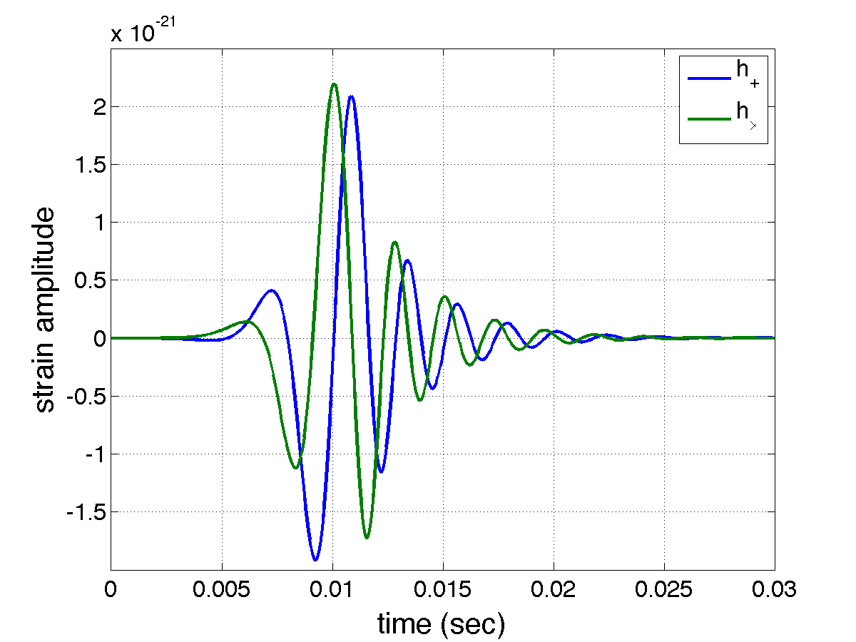
Figure 1: Time-series Lazarus waveforms [43] used for our simulations, from a nominal distance of 240 Mpc.

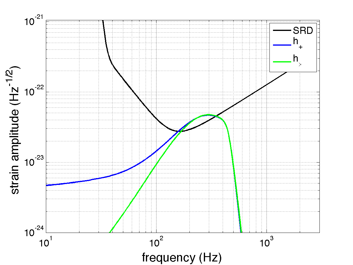
Figure 2: Strain-equivalent noise amplitude spectral density of the simulated data used in our tests (black) with spectra of the Lazarus waveforms [43] at 240 Mpc. The Lazarus spectra have been rescaled by $T^{-1/2}=(128/\mathrm{sec})^{1/2}$ to render them into the same units as the noise spectrum.

For the Bayesian statistic we adapt the broad-band signal prior (36)–(38) for each polarization. Specifically, we assume the simple model of a burst whose spectrum is white, with characteristic strain amplitude $\sigma$ at the Earth and duration equal to our chosen FFT length:

$$G = 2M$$ (76)

$$\mathbf{A} = \sigma^{2}\mathbf{I}$$ (77)

$$\mathbf{W} = \mathbf{I}\,.$$ (78)

We use a uniform prior on the signal arrival time $\tau$, and an isotropic prior on the sky position $(\theta,\phi)$. The Bayesian statistic was computed for approximately logarithmically spaced discrete values of characteristic strain $\sigma=10^{-23},3\times 10^{-23},10^{-22},3\times 10^{-22},10^{-21}$, and averaged together in post-processing. This averaging approximates a single Bayesian statistic with a Jeffreys (scale invariant) prior $p(\sigma)\propto 1/\sigma$ between $10^{-23}$ and $10^{-21}$. (Performing the combination in post-processing allowed us to maintain compatibility with the existing architecture of X-Pipeline; we do not use the $\sigma^{-4}$ prior from (43) because we are injecting from a fixed distance, not a spatially uniform population.)

Each likelihood statistic was computed over a fixed frequency band of [64,1088] Hz, with an FFT length of 1/128 sec. We analyzed blocks of data, overlapping by 75% of their duration. The detection probability as a function of false alarm probability is shown in Fig. 3. The distance used for the Lazarus simulations for this figure was $240/2.5=96$ Mpc; injections at other distances yielded similar results. At this distance, the total SNR deposited in the network $\sqrt{\sum_{\alpha}\mathrm{SNR}^{2}}$ was in the range $\sim 1-8$ with a mean value of 5, where

$$\sum_{\alpha}\mathrm{SNR}^{2}_{\alpha}=\sum_{\alpha}4\int_{0}^{\infty}\!\!df\,\frac{\left|F_{\alpha}^{+}\tilde{h}_{+}(f)+F_{\alpha}^{\times}\tilde{h}_{\times}(f)\right|^{2}}{S(f)}$$ (79)

and $S(f)$ is the one-sided noise power spectral density of each interferometer.

Fig. 3 is the receiver-operating characteristic plot for each of the statistics considered. The vertical axis represents the fraction of a population of signals whose detection statistics exceed the threshold that would only be crossed by background noise at the rate given by the false alarm probability on the horizontal axis. For example, we can read off the figure that if we can afford a false alarm probability of $10^{-2}$, the various detection statistics are able to detect between $0.4$ and $0.6$ of the injected signals. We see that the best performance is achieved by the Bayesian method with the $\sigma$ value most closely matching the injected signals, with the marginalized curve performing almost identically. The detection probability of the marginalized Bayesian method is significantly better than that of any of the non-Bayesian methods (standard likelihood, soft constraint, and hard constraint likelihoods) over the full range of false-alarm probabilities tested.

For a given false-alarm probability, we may compute the distance at which each likelihood achieves 50% efficiency by fitting a sigmoid curve to the simulations. The observed volume, and therefore the expected rate of detections for a uniformly distributed source population, scales as the cube of the distance. We computed the distance and volume for each statistic for two false alarm probabilities, $10^{-5}$ in Table 1 and $1/256\approx 3.9\times 10^{-3}$ in Table 2. As we compute 512 statistics per second, these correspond to false alarm rates of 1/200 Hz and 2 Hz respectively (as the statistics are computed on 75% overlapped data, these estimates are conservative). These rates are practical for event generation at the first stage of an untriggered (all-sky, all-time) burst search [44, 45, 5, 46]. At both of these false alarm probabilities, the Bayesian method can detect sources approximately 15% more distant, and consequently has an observed volume and expected detection rate approximately 50% greater, than the non-Bayesian statistics.

It is important to note that we do not use detailed knowledge of the signal waveform for the Bayesian analysis. Our prior is that the signal spectrum is flat over the analysis band ([64,1088] Hz), and by imposing no phase structure or sample-to-sample correlations we are assuming that over the integration time (1/128 sec) the time samples of strain are independently and identically distributed. Considering Figures 1 and 2, it is clear that these priors are not particularly accurate models for the actual gravitational-wave signal. Nevertheless, our Monte Carlo results demonstrate that even this incomplete prior information can improve the sensitivity of the search.

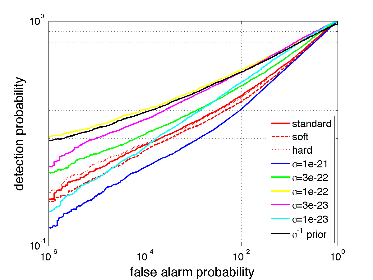
Figure 3: Receiver-operating characteristic (ROC) curves for the Bayesian, standard (Gürsel-Tinto), soft constraint, and hard constraint likelihoods for sources at 96 Mpc. The curve for a $\sigma^{-1}$ prior is obtained by marginalizing over probabilities associated with the discrete $\sigma$ values tested. The best performance is achieved by the $\sigma$ value most closely matching the amplitude of the injected signals, with the marginalized curve performing almost identically. The detection probability of the marginalized Bayesian method is significantly greater than that of any of the non-Bayesian methods (standard/Gürsel-Tinto, soft constraint, and hard constraint likelihoods) over the full range of false-alarm probabilities tested.

Table 1: Distances for false-alarm probability $10^{-5}$

Statistic	Distance (Mpc)	Distance (rel.)	Volume (rel.)
Standard	72.1	1.01	1.02
Soft	71.6	1.00	1.00
Hard	72.5	1.01	1.04
Bayesian	82.0	1.15	1.50

Table 2: Distances for false-alarm probability $1/256$

Statistic	Distance (Mpc)	Distance (rel.)	Volume (rel.)
Standard	87.1	1.03	1.08
Soft	84.9	1.00	1.00
Hard	86.9	1.02	1.07
Bayesian	97.9	1.15	1.53

4 Conclusions and Future directions

We have presented a comprehensive Bayesian formulation of the problem of detecting gravitational wave bursts with a network of ground-based interferometers. We demonstrated how to systematically incorporate prior information into the analysis, such as time-frequency or polarization content, source distributions and signal strengths. We have also seen that this Bayesian formulation contains several previously proposed detection statistics as special cases.

The Bayesian methodology we have derived to address the problem of detecting poorly-understood gravitational wave bursts yields a novel statistic. On theoretical grounds we expect this statistic to outperform previously proposed statistics. A Monte-Carlo analysis confirms this expectation: over a range of false alarms rates, the Bayesian statistic can detect sources at 15% greater distances and therefore observe 50% more events.

The Bayesian search requires explicitly adopting a model for the poorly understood signal. This is not a shortcoming. The model may be agnostic with respect to many features of the waveform. As we have demonstrated, existing methods are not free from their own signal models, but implicitly assume priors on the energies and spatial distribution of sources.

Coherent analyses of any kind are relatively costly, and efficient implementations must be sought. By specifying the problem as an integral, the Bayesian approach lets us leverage the extensive literature on numerical integration for techniques to accelerate the computation; one promising contender is importance sampling.

As second practical issue that must be dealt with is that the background noise of real gravitational wave detectors contains transient non-Gaussian features (“glitches”). As in the case of detection statistics, several ad hoc non-Bayesian statistics have been proposed to distinguish glitches from gravitational wave signals (see for example [30, 29]). Again, Bayesian methodology provides us with a direction in which to proceed: augment the noise model to better reflect “glitchy” reality, and to the extent we are successful, robustness will automatically follow.

5 Acknowledgments

We would like to thank Shourov Chatterji, Albert Lazzarini, Soumya Mohanty, Andrew Moylan, Malik Rakhmanov, and Graham Woan for useful discussions and valuable comments on the manuscript. This work was performed under partial funding from the following NSF Grants: PHY-0107417, 0140369, 0239735, 0244902, 0300609, and INT-0138459. A. Searle was supported by the Australian Research Council and the LIGO Visitors Program. For M. Tinto, the research was also performed at the Jet Propulsion Laboratory, California Institute of Technology, under contract with the National Aeronautics and Space Administration. M. Tinto was supported under research task 05-BEFS05-0014. P. Sutton was supported in part by STFC grant PP/F001096/1. LIGO was constructed by the California Institute of Technology and Massachusetts Institute of Technology with funding from the National Science Foundation and operates under cooperative agreement PHY-0107417. This document has been assigned LIGO Laboratory document number LIGO-P070114-00-Z.

6 References

References

- [1] http://www.geo600.uni-hannover.de/.
- [2] http://www.ligo.caltech.edu/.
- [3] http://tamago.mtk.nao.ac.jp/.
- [4] http://www.virgo.infn.it/.
- [5] B. Abbott et al. Astrophys. J., 681:1419, 2008.
- [6] É. É. Flanagan and S. A. Hughes. Phys. Rev. D, 57:4535, 1998.
- [7] É. É. Flanagan and S. A. Hughes. Phys. Rev. D, 57:4566, 1998.
- [8] F. Pretorius. Phys. Rev. Lett., 95:121101, 2005.
- [9] J. G. Baker, J. Centrella, D. Choi, M. Koppitz, and J. van Meter. Phys. Rev. Lett., 96:111102, 2006.
- [10] M. Campanelli, C. O. Lousto, P. Marronetti, and Y. Zlochower. Phys. Rev. Lett., 96:111101, 2006.
- [11] P. Diener, F. Herrmann, D. Pollney, E. Schnetter, E. Seidel, R. Takahashi, J. Thornburg, and J. Ventrella. Phys. Rev. Lett., 96:121101, 2006.
- [12] F. Herrmann, D. Shoemaker, and P. Laguna. 2006.
- [13] F. Loffler, L. Rezzolla, and M. Ansorg. 2006.
- [14] M. Shibata and K. Taniguchi. Phys. Rev. D, 73:064027, 2006.
- [15] T. Zwerger and E. Muller. Astron. Astrophys., 320:209, 1997.
- [16] H. Dimmelmeier, J. Font, and E. Muller. Astron. Astrophys., 393:523, 2002.
- [17] C. Ott, A. Burrows, E. Livne, and R. Walder. Astrophys. J., 600:834, 2004.
- [18] M. Shibata and Y. I. Sekiguchi. Phys. Rev. D, 69:084024, 2004.
- [19] C. D. Ott, A. Burrows, L. Dessart, and E. Livne. Phys. Rev. Lett., 96:201102, 2006.
- [20] P. Mészáros. Ann. Rev. Astron. Astrophys., 40:137, 2002.
- [21] C. Cutler and K. S. Thorne. 2002.
- [22] Y. Gursel and M. Tinto. Phys. Rev. D, 40:3884, 1989.
- [23] M. Tinto. In Proceedings of the International Conference on Gravitational Waves: Source and Detectors. World Scientific (Singapore), 1996.
- [24] W. G. Anderson, P. R. Brady, J. D. E. Creighton, and É. É. Flanagan. Phys. Rev. D, 63:042003, 2001.
- [25] M. Rakhmanov. Class. Quant. Grav., 23:S673, 2006.
- [26] T. Z. Summerscales, A. Burrows, L. S. Finn, and C. D. Ott. The Astrophysical Journal, 678:1142, 2008.
- [27] S. Klimenko, S. Mohanty, M. Rakhmanov, and G. Mitselmakher. Phys. Rev. D, 72:122002, 2005.
- [28] S. Mohanty, M. Rakhmanov, S. Klimenko, and G. Mitselmakher. Class. Quant. Grav., 23:4799, 2006.
- [29] L. Wen and B.F. Schutz. Class. Quantum Grav., 22:S1321, 2005.
- [30] S. Chatterji, A. Lazzarini, L. Stein, P. Sutton, A. Searle, and M. Tinto. Phys. Rev. D, 74:082005, 2006.
- [31] J. Sylvestre. Phys. Rev. D, 68:102005, 2003.
- [32] N. Arnaud, M. Barsuglia, M. Bizouard, V. Brisson, F. Cavalier, M. Davier, P. Hello, S. Kreckelbergh, and E. K. Porter. Phys. Rev. D, 68:102001, 2003.
- [33] L. S. Finn. 1997.
- [34] B. Allen, J. D. E. Creighton, . . Flanagan, and J. D. Romano. Phys. Rev. D, 67:122002, 2003.
- [35] E. T. Jaynes. Probability Theory: The Logic of Science. Cambridge University Press, 2003.
- [36] P. Gregory. Bayesian Logical Data Analysis for the Physical Sciences. Cambridge University Press, 2005.
- [37] M. Principe and I. Pinto. Class. Quant. Grav., 25:075013, 2008.
- [38] A. C. Searle, P. J. Sutton, M. Tinto, and G. Woan. Class. Quant. Grav., 25:114038, 2008.
- [39] I S Heng. Class. Quant. Grav., 26:105005 (9pp), 2009.
- [40] S. Klimenko, S. Mohanty, M. Rakhmanov, and G. Mitselmakher. J. Phys. Conf. Ser., 32:12, 2006.
- [41] https://geco.phys.columbia.edu/xpipeline/wiki.
- [42] F. Beauville et al. J.Phys.Conf.Ser., 32:212, 2006.
- [43] J. Baker, M. Campanelli, C. O. Lousto, and R. Takahashi. Phys. Rev. D, 65:124012, 2002.
- [44] B. Abbott et al. Phys. Rev. D, 72:042002, 2005.
- [45] B. Abbott et al. Phys. Rev. D, 77:062004, 2008.
- [46] B. Abbott et al. Class. Quantum Grav., 24:5343, 2007.