Late stage, non-equilibrium dynamics in the dipolar Ising model

Abstract

Magnetic domain structures are a fascinating area of study with interest deriving both from technological applications and fundamental scientific questions. The nature of the striped magnetic phases observed in ultra-thin films is one such intriguing system. The non-equilibrium dynamics of such systems as they evolve toward equilibrium has only recently become an area of interest and previous work on model systems showed evidence of complex, slow dynamics with glass-like properties as the stripes order mesoscopically. To aid in the characterization of the observed phases and the nature of the transitions observed in model systems we have developed an efficient method for identifying clusters or domains in the spin system, where the clusters are based on the stripe orientation. Thus we are able to track the growth and decay of such clusters of stripes in a Monte Carlo simulation and observe directly the nature of the slow dynamics. We have applied this method to consider the growth and decay of ordered domains after a quench from a saturated magnetic state to temperatures near and well below the critical temperature in the two dimensional dipolar Ising model. We discuss our method of identifying stripe domains or clusters of stripes within this model and present the results of our investigations.

1 Introduction

The properties of ultra-thin magnetic thin films have been the subject of study for some time, but new experimental techniques to create and probe such systems has intensified the efforts of researchers to understand these systems in recent years.[1, 2, 3] Among the more interesting properties is the existence of stripe phases. These phases are the result of the competition between short-range exchange interactions and long-range, dipole-dipole interactions. Such pattern formation is of great interest as the foundations of future potential magnetic storage devices are based in part on the properties of such materials.[4] However, the phenomena is much more general and similar patterns have been observed in such diverse systems as Langmuir monolayers, diblock co-polymers, and type 1 superconductors.[5] More recently similar competition between long-range, dipole-dipole and short-range interactions has been seen in model systems as an essential control mechanism in the self assembly process for nano-structures.[6]

The static, equilibrium properties of ultra-thin magnetic films have been well studied experimentally [2] and the dipolar Ising model has been considered extensively in efforts to explain these properties.[7] However a better understanding of the stability and dynamics of the domain structures in these materials is still needed and is highly desirable given that they determine many of the technologically important properties of these materials. It is widely known that the static and dynamic properties of a material can sometimes be determined by clusters or domains within the material. Such is the case the two-dimensional Ising model with short range interactions only[8], where the explicit connection between the geometric clusters of spins in the same state to the physical clusters which are characteristic of the critical phenomena in the system, has been formally established.[9, 10] This connection has been exploited to gain a better understanding of the dynamics of the short range interaction Ising spin system, the nature of the phase transition, and also to develop acceleration algorithms for Monte Carlo simulations, which have greatly expanded the utility of the model.[11, 12] A similar connection has yet to be established for the dipolar Ising model. Given the potential utility of the dipolar Ising model, and given the very slow dynamics that have observed in simulations to date, such a connection and the development of acceleration algorithms would be quite useful. The methods and results presented in this work are an initial step toward the development of such an algorithm and at the same time provide insight in to the dynamics of the dipolar Ising model itself.

1.1 The dipolar Ising model

The Hamiltonian for the dipolar Ising model in reduced units can be written as

$${\cal{H}}=-J\sum_{<ij>}\sigma_{i}\sigma_{j}+g\sum_{i,j}\sigma_{i}\Gamma_{ij}\sigma_{j}+H\sum_{i}\sigma_{i}$$ (1)

where $<i,j>$ in the first term indicates a sum over all pairs of nearest neighbor spins $i,j$, $\sigma_{i}=\pm 1$ is the magnetic moment at site $i$ and $J$ is the strength of the exchange interaction. The second term is a long-range dipole-dipole interaction of strength $g$ and the sum is over all pairs of spins. The final term treats the interaction with an applied field, $H$, which we do not consider in this work. The system is assumed to be infinite, but restricted to states which are periodic. Periodic boundary conditions are therefore used to treat the exchange interaction and Ewald sums are used to account for the long-range nature of the dipolar interaction. The exact form of $\Gamma_{ij}$ and other details related to the Ewald summation are as given by Ref. [13]. In this paper we assume the spins are perpendicular to the plane of the film.

1.2 Previous work

The equilibrium properties of dipolar Ising model have been studied extensively and a review of this work can be found in De’Bell et al. [7] and the works cited therein. In the work presented here the ratio of $J$ to $g$ has been fixed at $J/g=8.9$, which has been shown previously to lead to an ordered ground state, in a monolayer, of stripes of width 8 spins parallel to a lattice axis.[14] The nature of this transition is still the subject of some debate, much of which centers on the characteristics of the equilibrium phase just above the critical temperature and the comparison to experimental results.

In contrast the non-equilibrium dynamics of the dipolar Ising model have not been so extensively considered. The earliest work considered the relaxation of the magnetization from the saturated magnetic state, ($\{\sigma_{i}\}=1$), after a quench toward equilibrium at a temperature below $T_{c}$. Sampaio, de Albuquerque and de Menezes[15] found that depending on the relative strengths of the dipolar and exchange interactions, one can have either exponential or power-law relaxation. The time frame considered was very short, typically on the order of 5000 Monte Carlo steps (MCS) at most, and the relative strength of the interactions was such that the stripe width in the ground state was limited to at most 4 spins. Rappoport et al.[16] reported similar results on larger lattices, but with a truncated dipolar interaction.

The phenomena of aging in the dipolar Ising model was considered in a number of articles, all of which considered small stripes of width one or two spins. By measuring the spin auto-correlation function,

$$C(t,t_{w})=\frac{1}{N}\sum_{i}\left<\sigma_{i}(t+t_{w})\sigma_{i}(t_{w})\right>,$$ (2)

Toloza, Tamarit and Cannas [17] were able to observe aging, the nature of which was dependent on the relative strength of the interactions. Stariolo and Cannas[18] expanded upon this earlier work to show how $C(t,t_{w})$ crosses over from logarithmic decay to algebraic decay as the ground state stripe width increases. Gleiser et al. [19] and Gleiser and Montemurro [20] measured the time evolution of the domain size of stripes of width one and two spins and hypothesized that the differences in the nature of the dynamics was related to the existence of metastable states. All of these studies were concerned with short to intermediate time scales (up to $t=10^{6}$) and only for the case of small stripe widths.

Bromley and his co-authors[21, 22] considered the dynamics of systems with a larger stripe width (8 spins) during a quench from the saturated magnetic state toward equilibrium near the critical temperature. They were able to establish the existence and character of three relaxation regimes. They considered results from simulations on the order of at most 1,000,000 Monte Carlo steps (MCS), to develop a general understanding of the relaxation in their system in each of three regimes that they identified. At very early times they found that the dynamics of the system was characterized by the nucleation of small islands, where the spins are oriented in the direction opposite to the initial saturation direction. As these small islands grew the net magnetization approached zero. In the second regime there remained a small remnant magnetization. This remnant magnetization decays at a rate which is much slower than that in the first regime. In the final regime, at late times, they found that the islands become elongated and arranged into regions which manifest the stripe pattern of the expected equilibrium phase. However these local regions did not yet share a common orientation and hence the system was not completely in the smectic phase. To support this conjecture, they provided three snapshots of an extended simulation that showed single spin configurations at times $t=300,000$, $t=600,000$ and $t=900,000$, where by hand they determined the regions of local smectic ordering. Their results were consistent with those of Desai and Roland and Sagui and Desai who had conducted similar studies using Langevin dynamics for a model with a continuous uniaxial “spin” variable, with an additional significant difference being the use of open boundaries.[23, 24]

Mu and Ma [25] considered a dipolar model system under going a quench from a random state. They discussed qualitatively the early stages of the relaxation to equilibrium, and felt that the depth of the quench fundamentally changed the nature of the relation process. Their simulations were run for times on the order of 100,000 MCS for stripes of various width from approximately 1 to 9 spins. For a deep quench they claimed that the labyrinth structure they observed became frozen due to the frustration induced by the competition between the short- and long-range interactions.

It is the late stage relaxation identified by Bromley and Mu and Ma, but which was not considered in depth due to computer time constraints, that we wish to address in this article. We also wish to consider ground state stripes of the size treated by Bromley and by Mu and Ma, rather than the very small stripes considered in the other works discussed above. We have extended the length of simulation by at least a factor of 10 compared to previous studies, and have recorded the spin configurations every 1000 MCS.[26] Our simulations have a run length of between 2 million and 14 million Monte Carlo time steps, depending on the temperature of the simulation. The longest of our simulations required over 30 days to run using a 4 way parallel code on 4 CPU’s. Thus this single simulation required 120 days of CPU time. Because of this huge computational demand we have only considered a few temperatures and conducted two sets of simulations at each temperature. However even this small number of simulations required over 4 years of CPU time.

While we will be drawing analogies between the standard 2D Ising model and the dipolar Ising model, one must remember that unlike the standard 2D Ising model, the ordering observed in the dipolar Ising model is a mesoscopic ordering of the stripes and not a microscopic ordering of the spins themselves. Therefore one must be cautious about characterizing the transition in terms of spin properties rather than in terms of properties of the stripes. For stripes of small width this can be a serious concern as the spins fluctuations and the stripe fluctuations can occur on similar length scales. For example, if one were to consider a system with stripes of width h=2, a spin flip would be equivalent to half the width of a stripe and even in the ground state of the system 100% of the spins would lie on a stripe boundary. If instead one where to consider a system with a ground state of stripes of width h=8 (or greater), then only 25% of spins lie on a boundary in the ground state and a single spin flip is no longer comparable to the excitation required to disorder the mesoscopic stripe order. This is also important as the smallest of ground state stripe widths seen experimentally is still quite large, typically on the order of 100-1000 spins.[27, 28] Thus $h=8$ must be considered small when comparing to experimental system, however it is hoped that scaling arguments can be developed which will allow meaningful comparisons to be made.[29]

To study the dynamics and more precisely the late stage relaxation of this system we need to be able to define domains within the system which are based, not on the state of the spins, but on the local orientation of the stripes. It is important to note the distinction between clusters of spins or spin domains and clusters of stripes or stripe domains. A stripe is in fact a geographical domain within which the spins are in the same state and therefore a stripe may be referred to as a spin domain or a cluster of spins. A stripe domain, or equivalently a cluster of stripes, will be a geographical domain in a striped system within which the stripes share an orientation. It will be the evolution of these stripe domains or clusters of stripes which should define the dynamics of our system.

The rest of this paper proceeds as follows: Section 2 discusses the method used to define the clusters of stripes in the model system and provides some sample configurations. Section 3 discusses the results of our simulations in terms of the time evolution of the magnetization and the order parameter. Section 4 reanalyzes the same simulations by measuring the properties of stripe domains defined using our method of section 2. Finally section 5 summarizes the results.

2 Identifying clusters by stripe orientation

To achieve the goals of this work we need to be able to identify, within a given spin configuration, domains where the stripes have a particular orientation, along either the $x$-axis or the $y$-axis of the underlying lattice. We also need the algorithm to be simple and efficient. The standard methods for such an analysis are based on the work of M. Seul, L. O’Gorman and M. Sammon [30], which were developed in part to support their research related to pattern formation in numerous experimental systems[5] including some novel magnetic systems.[31, 32] We have implemented and used some of those routines to aid in our analysis. However those routines are quite general and we have developed efficient routines specifically for our purposes. In future work we will systematically compare our results to those that can be obtained using the routines of Seul, O’Gorman and Sammon.

As a first step in our method we will make use of a simple line-of-sight argument. For each spin in the system assume that one is sitting at the spin location in the lattice. Now look in each of the four directions along the lattice axes ($+x$, $-x$, $+y$ and $-y$) and determine how far in each direction one would walk before encountering a spin in the opposite state. Now add the length one finds in the $+x$ and $-x$ directions together and the length one finds in the $+y$ and $-y$ directions together. If the former length is larger than the latter length ( $x$ length is larger than $y$ length) then assume that spin location is part of a region with stripes oriented along the $x$-axis. If the opposite is true ($y$ length is larger than $x$ length) then one assumes the spin is located in a region with stripes oriented along the $y$-axis. Thus one can assign to each point on the lattice a binary variable which designates the orientation of the stripes at that point on the lattice. For example, Figure 1a shows a spin configuration taken from a simulation just below the critical temperature, but before the system has reached equilibrium. The system size is $256\times 256$, but to highlight the nature of the stripe domains given the periodic boundary conditions, we have tiled 4 copies of the system together to give a $512\times 512$ picture. In this Figure red (gray) indicates spins with $\sigma=+1$ and blue (black) indicates spins with $\sigma=-1$. Figure 1b shows how our the line of sight algorithm would classify each point in the system. In this Figure green (black) represents points where the systems appears to be ordered vertically (along the y-axis) and yellow (gray) represents horizontally ordered regions (along the x-axis).

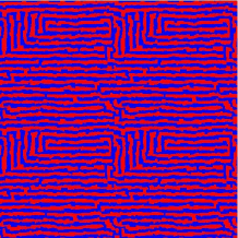
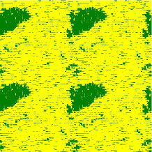
Figure 1: (a) Original spin configuration from a $256\times 256$ simulation tiled to provide a $512\times 512$ image. Red(gray):$\sigma=+1$, Blue(black):$\sigma=-1$ (b) The result of applying the first stage of our cluster finding method. Green (black):local vertical stripes. Yellow(gray):local horizontal stripes.

It is quite evident from Figure 1b that our routine does a reasonable job determining the stripe orientation however, spin fluctuations can lead to patchiness in the classification. These artifacts are difficult to avoid and are unimportant when one is concerned with the nature of the ordering in the system, as they reflect microscopic fluctuations and we are concerned with a mesoscopic scale ordering. To provide a clearer picture of the ordered regions we therefore employ a median filter to our initial classified image array. The purpose of such a filter is to reduce speckle noise, and functions by replacing the value at a site by the median value in a $k\times k$ neighborhood centered on that site. As we allow only two states in our image, the median filter reduces to a “majority rules” calculation. The choice of $k$ is the only free parameter in this filter and we show in Figure 2 three examples of this filter applied to our initial classified image. In Figure 2a-c we have taken $k=3$, $k=7$, and $k=15$ which are equal to just below one half of a stripe width, just below one stripe width, and just below than two stripe widths. In Figure 3 we have superimposed the boundaries of the stripe domains shown in 2b on to the original spin configuration.

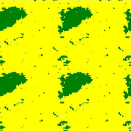
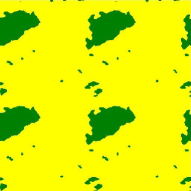
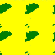
(a)$k=3$	(b)$k=7$	(c)$k=15$

Figure 2: The result of applying a median filter to the image shown in Figure 1b with $k$ equal to (a) 3, (b) 7 and (c) 15. Green (black):local vertical stripes. Yellow(gray):local horizontal stripes.

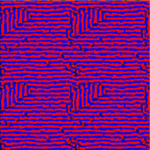
Figure 3: The clusters of horizontal and vertical stripes in Figure 1a defined after the application of a median filter using $k$ equal 7 as in Figure 2b. The black lines divide regions with horizontal and vertical stripe orientations.

As one can see the median filter has the desired effect of reducing speckle noise and does not effect the underlying classification in any significant manner. For the purposes of this work we have chosen to use $k=7$, which, as stated above, is just below the stripe width in the ground state. Thus small spin-level fluctuations do not influence our results, while larger stripe-level fluctuations will.

3 Magnetization and Order Parameter

3.1 Magnetization

We wish to study the late stage dynamics of a quench from the saturated magnetic state, $M=1$, to equilibrium at temperatures below the critical temperature in the dipolar Ising model. The early time dynamics have been considered previously by a number of authors as discussed above.

As stated above for our chosen ratio the ground state stripe width is $h=8$ spins. Most previous work considered systems where the ground state was stripes of width 1 or 2 spins. The advantage of choosing such small stripes was that the dynamics, while still much slower than what is typical for the 2D Ising model, are still accessible within a reasonable length simulation. We do not expect our results for wider stripes to necessarily be comparable to these studies of very narrow stripes, but instead hope they will be qualitatively similar to experimental results. It has been shown that the model system we have chosen has a critical temperature of approximately $T_{c}=5.0\pm 0.1$. Therefore we have chosen to simulate quenches below $T_{c}$ at $T=4.00,4.25,4.50,4.75$ and $4.90$, at $T=T_{c}=5.00$ and just above $T_{c}$ at $T=5.10$, and $5.20$. The variation of the magnetization as a function of time has been well studied by Bromley et al. for exactly the system considered in this work. They showed that for all the temperatures they considered the magnetization decayed to within %1 of the saturated magnetization after about 2000 MCS, however they also showed that some memory of the original saturated state remains for a much longer time period. Our results, at all temperatures considered, are in agreement with those of Bromley et al., and show that the magnetization decays effectively to zero within the first 2000 MCS.

3.2 Order Parameter

As pointed out by Bromley et al. the system has not reached equilibrium, within the time frame they considered. They were able to conclude this because the system should be in a smectic striped phase, but direct observation of the spin configurations clearly showed a system in the tetragonal phase. Bromley et al. also used properties of the magnetization to show that the system had not yet reached equilibrium. We are able to show this more directly and quantitatively by calculating the orientationial order of the system. To do so we calculate the orientational order parameter, $O_{hv}(t)$, defined by Booth et al.[13] as

$$O_{hv}=\frac{n_{h}-n_{v}}{n_{h}+n_{v}},$$ (3)

where $n_{h}$ and $n_{v}$ are the number of bonds between spins with opposite orientation which are parallel to the horizontal or vertical direction, respectively. We have also calculated an alternative, more general, order parameter, recently proposed by Tan and MacIsaac[33] based on the structure factor. For our model system in equilibrium below $T_{c}$ there are two main peaks in the structure factor, $S(\vec{q})$. These peaks are along one set of the axes in q-space, characteristic of stripes parallel to one of the axes in real space; either $x=0$ or $y=0$. Above $T_{c}$ there are four main peaks in $S(\vec{q})$, as one has stripes along both axes in real space. If one defines $\vec{q}_{+}$ and $\vec{q}_{-}$ as the location of the main peaks in q-space associated with stripes along $x=0$ and $y=0$ respectively, then one can define a general order parameter,

$$O_{\pm}=\frac{S(\vec{q}_{+})-S(\vec{q}_{-})}{S(\vec{q}_{+})+S(\vec{q}_{-})},$$ (4)

which will be non-zero below $T_{c}$ with a saturation value of plus or minus one and zero above. This order parameter has the benefit of being more general that $O_{hv}$ as it can be defined even in the case where the stripes are not parallel to a lattice axis. Note that we have measured $|O_{\pm}|$ and $|O_{hv}|$ in our simulations, which is appropriate in a finite system.[34]

In Figures 4, 5, 6, and 7 we show both $\left|O_{hv}\right|$ and $\left|O_{\pm}\right|$ at $T=4.00,4.25,4.90$   and   $5.00$ respectively from a single quench at each temperature. It is important to note that these are from single simulations with no averaging and therefore we are generally looking at qualitative features. Figures 4 to 7 are for temperatures below or at $T_{c}$ and show very similar features, although they have different times scales.

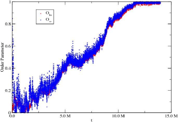
Figure 4: Order parameters as a function of time in MCS for a quench from the saturated magnetic state, $M(0)=1$, to $T=4.00$.

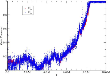
Figure 5: Order parameters as a function of time in MCS for a quench from the saturated magnetic state, $M(0)=1$, to $T=4.25$.

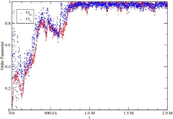
Figure 6: Order parameters as a function of time in MCS for a quench from the saturated magnetic state, $M(0)=1$, to $T=4.90$.

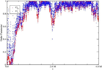
Figure 7: Order parameters as a function of time in MCS for a quench from the saturated magnetic state, $M(0)=1$, to $T=5.00$.

In each simulation at each temperature there are three stages or regimes. The order parameter starts at zero, as it should be in the initial, ferromagnetic state, and remains near zero at early times. For $T=4.00$ and $4.25$ this stage can be up to 2 million to 4 million MCS, while at $T=4.90$ and $T=5.00$ it is considerably shorter; on the order of 100,000 MCS. After this stage the order parameter begins to grow over a time period which is again temperature dependent, until it saturates at its equilibrium value. At this point the system has reached equilibrium and fluctuates about its equilibrium value. We can estimate when the system reaches equilibrium by measuring the time it takes the order parameter, $O_{hv}$, to first reach 99% of its equilibrium value. For the twelve runs, two at each of six temperatures below $T_{c}$, we can plot this value versus temperature as shown in Figure 8.

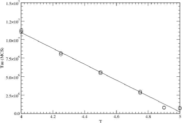
Figure 8: Estimate of the time $(\tau)$ in MCS for the order parameter, $|O_{hv}|$, to reach 99% of its equilibrium value as a function of the temperature of the simulation. The line is a least squares fit to the points shown and serves only as a guide to the eye.

One will note that below $T$ for all the temperatures considered the system does not “freeze” into a metastable tetragonal state as suggested by Mu and Ma, but rather the system continues to evolve slowly towards the equilibrium state, with a characteristic time that grows as a function of the depth of the quench. Once the system has reached equilibrium the order parameter fluctuates about its equilibrium mean value. In other words it does not appear that this characteristic time will diverge at finite temperature, so we find no evidence of a glass-like state. Above $T_{c}$ both order parameters show the system does not possess any significant orientational order as one would expect.

4 Cluster properties

Now we wish to determine if it is possible to qualitatively explain the non-equilibrium relaxation of the magnetization and the order parameter using the properties of the clusters of stripes identified using the methods introduced earlier. We will show configurations from a simulation at $T=4.00$ for illustrative purposes and discuss properties at all simulation temperatures.

Figure 9 shows the spin configuration from one simulated quench at $T=4.00$ at early times, t:(a) $t=1000$,(b) $t=2000$,(c) $t=10,000$ and (d) $t=100,000$. One can clearly see early dynamics similar to those described by Bromley et al., Cannas et al. and Mu and Ma. Initially there is nucleation of small spin clusters, which grow and transform into the labyrinth stripe patterns which are clearly evident at $T=4.00$ by $t=10,000$ in Figure 9c. This is consistent both with the magnetization we have measured and the results of the earlier studies. It is also consistent with the order parameter at early times, having a value very close to zero, as the stripes are just beginning to manifest themselves and hence there is no real orientational order. By $t=10,000MCS$ our cluster identification scheme is able to partition the system in to domains based on the stripe orientation and these clusters of stripes grow and coalesce with time until approximately $t=100,000$ MCS at $T=4.00$. At that point the size of the clusters of stripes are comparable to our system size. This is typically the regime that has been considered previously.

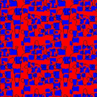
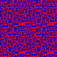
(a) $t=1,000$	(b) $t=2,000$
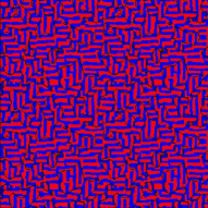
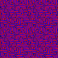
(c) $t=10,000$	(d) $t=50,000$
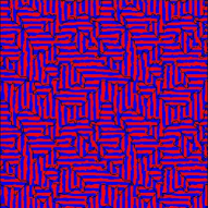
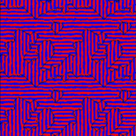
(e) $t=100,000$	(f) $t=500,000$

Figure 9: Configurations for a quench from a saturated magnetic state to $T/g=4.00$ at various times from one simulation.

Figure 10 shows the average size (mass) of the clusters of stripes in the simulation as a function of time in MCS from a single simulation at $T=4.00$.

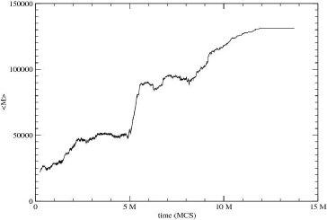
Figure 10: The average size (mass) of a cluster of stripes as a function of time in MCS at $T=4.00$.

This average includes both horizontal and vertical stripe clusters. The different dynamical regimes are clearly seen in this Figure. The initial regime has ended after at most $200,000$ MCS. The intermediate regime, from $t=200,000$ to $t=11,000,000$ occurs when the system has phase separated into a few very large stripe domains. Spin configurations from this region are shown in Figure 11.

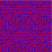
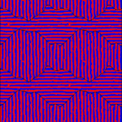
(a) $t=1,000,000$	(b) $t=2,000,000$
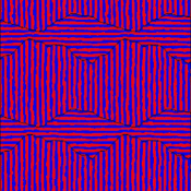
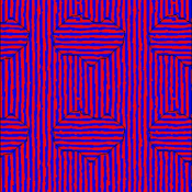
(c) $t=5,000,000$	(d) $t=6,000,000$
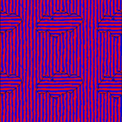
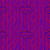
(e) $t=8,000,000$	(f) $t=9,000,000$
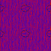
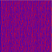
(g) $t=10,000,000$	(h) $t=14,000,000$

Figure 11: Configurations for a quench from a saturated magnetic state to $T/g=4.00$.

The feature in Figure 10 at approximately $t=5\mbox{ million}$ MCS is an artifact of the last cluster of horizontal stripes no longer spanning the system, such that instead of counting as 2 clusters in our tiled system it counts as 4 half size clusters. At that time the system consists of a majority phase with a single stripe domain of the minority stripe phase embedded within it. The dynamics of the system is now defined by the slow evaporation of this domain, which occurs as defects in the stripes are removed from the system. These defects occur along the boundary of the last cluster of stripes of the minority phase. To show this we measure the mass of the largest cluster of the minority stripe phase as a function of time. In Figure 12 we show the mass in the time frame from $t=5\mbox{ million}$ to $t=14\mbox{ million}$. Again as this is data from a single run rather than an ensemble average from many runs, one is looking at the qualitative behavior of the system rather than trying to extract the functional form of the decay.

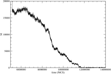
Figure 12: The size (mass) of the last cluster of the minority stripe phase as a function of time in MCS at $T=4.00$. In the time frame shown there is only one cluster of the minority stripe phase.

5 Summary

In summary we have shown how to simply and efficiently define clusters of stripes within the dipolar Ising model based on the local stripe orientation and have tracked the growth and decay of such clusters during a quench from a saturated magnetic state to a number of temperatures below the critical temperature. We have considered the non-equilibrium relaxation by observing the time dependence of both the magnetization and order parameter and by observing the time dependence of these stripe domains. We have confirmed earlier results concerning the early and intermediate stages of this relaxation and have provided the longest simulations to date to allow the study of the late stage relaxation. Our results indicate that the late stage relaxation is dominated by the very slow evaporation of clusters of the minority stripe phase. In all cases we have found that the system relaxes into the smectic, striped ground state with no indications of freezing into a spin-glass-like state.

This work was supported by the Natural Sciences and Engineering Council of Canada (NSERC). The authors would like to acknowledge SHARCNET, for the provision of the computing resources used in this work.

References

- [1] G. A. Prinz, Science 282 (1998) 1660.
- [2] B. Heinrich, J.A.C. Bland (Eds.), Ultrathin Magnetic Structures, Springer-Verlag, Berlin, 2004.
- [3] J. Shen, Z. Gai, J. Kirschner, Surf. Sci. Rep. 52 (5-6) (2004) 163–218.
- [4] S. A. Wolf, D. D. Awschalom, R. A. Buhrman, J. M. Daughton, S. von Molnár, M. L. Roukes, A. Y. Chtchelkanova, D. M. Treger, Science 294 (2001) 1488.
- [5] Michael Seul, David Andelman, Science 267 (1995) 476–483.
- [6] X. Zhang, Z.L. Zhang, S.C. Glotzer, Journal of Physical Chemistry C 111 (11) (2007) 4132–4137.
- [7] K. De’Bell, A. B. MacIsaac, J. P. Whitehead, Rev. Mod. Phys 72 (2000) 643.
- [8] Marco D’Onorio De Meo, Dieter W. Heermann, Kurt Binder, Journal of Statistical Physics 60 (5/6) (1990) 585–617.
- [9] A. Coniglio, W. Klein, J. Phys. A 13 (8) (1980) 2775–2780.
- [10] A. Coniglio, Correlations in Thermal and Geometrical Systems, in: Correlations and Connectivity, Vol. 188 of Series E: Applied Sciences, Kluwer Academic Publishers, The Netherlands, 1990, pp. 21–33.
- [11] R. H. Swendsen, J.S. Wang, Phys. Rev. Lett. 58 (2) (1987) 86–88.
- [12] U. Wolff, Phys. Rev. Lett. 62 (4) (1989) 361–364.
- [13] I. N. Booth, A. B. MacIsaac, J. P. Whitehead, K. De’Bell, Physical Review Letters 75 (5) (1995) 950–953.
- [14] A. B. MacIsaac, J. P. Whitehead, M. C. Robinson, K. De’Bell, Phys. Rev. B 51.
- [15] L. Sampaio, M. deAlbuquerque, F. deMenezes, Physical Review B 54 (9) (1996) 6465–6472.
- [16] T. Rappoport, S. Menezes, L. Sampaio, M. de Albuquerque, F. Mello, International Journal of Modern Physics C 9 (6) (1998) 821–825.
- [17] J. Toloza, F. Tamarit, S. Cannas, Physical Review B 58 (14) (1998) R8885–R8888.
- [18] D. Stariolo, S. Cannas, Physical Review B 60 (5) (1999) 3013–3016.
- [19] P. Gleiser, F. Tamarit, S. Cannas, M. Montemurro, Physical Review B 68 (13).
- [20] P. M. Gleiser, M. A. Montemurro, Physica A-Statistical Mechanics and its Applications 369 (2) (2006) 529–534.
- [21] S. Bromley, J. Whitehead, in: High Performance Computing Systems and Applications, Kluwer, 2000, p. 587.
- [22] S. Bromley, J. Whitehead, K. D’Bell, A. MacIsaac, Journal of Magnetism and Magnetic Materials 264 (2003) 14.
- [23] C. Roland, R. C. Desai, Phys. Rev. B 42 (10) (1990) 6658–6669.
- [24] C. Sagui, R. C. Desai, Phys. Rev. E 49 (3) (1994) 2225–2244.
- [25] Y. Mu, Y.-Q. Ma, Journal of Chemical Physics 117 (4) (2002) 1686.
- [26] Movies showing the entire evolution of the system are available via the author’s website at http://blue.beowulf.uwo.ca/Movies.
- [27] A. Bauer, G. Meyer, T. Crecelius, I. Mauch, G. Kaindl, Journal of Magnetism and Magnetic Materials 282 (Sp. Iss. SI) (2004) 252–255.
- [28] C. A. F. Vaz, J. A. C. Bland, G. Lauhoff, Reports on Progress in Physics 71 (5).
- [29] J. Whitehead, A. MacIsaac, Scaling properties in dipolar spin models, In preparation.
- [30] Michael Seul, Lawrence O’Gorman, Michael J. Sammon, Practical Algorithms for Image Analysis, Cambridge University Press, 2000.
- [31] M. Seul, R. Wolfe, Physical Review A 46 (12) (1992) 7519–7533.
- [32] M. Seul, R. Wolfe, Physical Review A 46 (12) (1992) 7534–7547.
- [33] T. Tan, A. B. MacIsaac, Journal of Physics-Condensed Matter 19 (45).
- [34] K. Binder, D. W. Heermann, Monte Carlo simulation in statistical physics, Springer-Verlag Series in Solid-State Sciences 80, 1992.