Eleven years of radio monitoring of the Type IIn supernova SN 1995N

Abstract

We present radio observations of the optically bright Type IIn supernova SN 1995N. We observed the SN at radio wavelengths with the Very Large Array (VLA) for 11 years. We also observed it at low radio frequencies with the Giant Metrewave Radio Telescope (GMRT) at various epochs within $6.5-10$ years since explosion. Although there are indications of an early optically thick phase, most of the data are in the optically thin regime so it is difficult to distinguish between synchrotron self absorption (SSA) and free-free absorption (FFA) mechanisms. However, the information from other wavelengths indicates that the FFA is the dominant absorption process. Model fits of radio emission with the FFA give reasonable physical parameters. Making use of X-ray and optical observations, we derive the physical conditions of the shocked ejecta and the shocked CSM.

1 Introduction

Type IIn supernovae (hereafter SNe IIn) show narrow H$\alpha$ emission line atop a broad emission feature, with no broad absorption. This classification was suggested by Schlegel (1990) who noticed the above properties in 8 supernovae (SNe). The H$\alpha$ and bolometric luminosities of most SNe IIn are large, which can be explained by the shock interaction of supernova (SN) ejecta with a very dense circumstellar (CS) gas (Chugai, 1990). Many SNe IIn also show an excess late time infrared emission, which is a signature of dense CS dust (Gerardy et al., 2002). CS interaction in SNe is typically observed by radio and X-ray emission (Chevalier & Fransson, 2003). However, in many cases, radio emission from SNe IIn has not been detected (Van Dyk et al., 1996).

One of the important issues for SNe IIn is their high presupernova mass loss rates. For example, for SN 1997ab the derived mass loss rate for a presupernova wind velocity of $90\,{\rm km\,s^{-1}}$ is $\sim 10^{-2}\,M_{\odot}\,{\rm yr^{-1}}$ (Salamanca et al., 1998). For SN 1994W the mass loss rate was $\sim 0.2\,M_{\odot}\,{\rm yr^{-1}}$ (Chugai et al., 2004), and for SN 1995G $\sim 0.1\,M_{\odot}\,{\rm yr^{-1}}$ (Chugai & Danziger, 2003). One possibility for these high mass loss rates is that they are related to an explosive event a few years before the SN outburst (Chugai & Danziger, 2003; Pastorello et al., 2007). Radio observations may put better constraints on the mass loss of the progenitor stars.

SN 1995N was discovered in MCG $-$02$-$38$-$017 (Arp 261) on 1995 May 5 (Pollas et al., 1995) at a distance of 24 Mpc (see Fransson et al., 2002). Pollas et al. (1995) estimated that the supernova was at least 10 months old upon discovery by comparing it with spectroscopic chronometers, and classified it as a Type IIn supernova. We assume the date of explosion to be 1994 July 4 throughout the paper (Fransson et al., 2002). SN 1995N turned out to be relatively bright at late times in most wavebands. It was detected in the radio with the Very Large Array (VLA, Van Dyk et al., 1996) and the Giant Metrewave Radio Telescope (GMRT, Chandra et al., 2005). In X-rays it was detected first by ROSAT in Aug 1996 and Aug 1997, and later by ASCA in Jan 1998 (Fox et al., 2000). In July 2003 XMM-Newton (Zampieri et al., 2005) and in March 2004 Chandra X-ray Observatory (Chandra et al., 2005) detected the late time X-ray emission from the SN. SN 1995N has declined very slowly in the optical band (Li et al., 2002; Pastorello et al., 2005), with only a 2.5 mag change in the V-band over $\sim 2500$ days after explosion. This is consistent with the slow spectral evolution reported in Fransson et al. (2002). Ground based optical and HST observations of the late-time spectral evolution of SN 1995N were used by Fransson et al. (2002) to argue that the late-time evolution is most likely powered by the X-rays from the interaction of the ejecta and the circumstellar medium of the progenitor. They in turn proposed that the progenitors of Type IIn supernovae are similar to red supergiants in their superwind phases, when most of their hydrogen-rich gas is expelled in the last $10^{4}\,\rm yr$ before explosion.

In this paper, we report extensive radio observations of SN 1995N taken with the VLA and GMRT. We discuss the observations and data analysis in §2. We fit various models to the data and discuss the results in §3. In §4, we utilize the results from other wavelength observations along with the radio bands to derive constraints on the physical parameters. We summarize our results briefly in §5.

2 Observations

2.1 VLA observations

The VLA followed SN 1995N for eleven years, from June 1995 until September 2006. The observations were taken at 22.48 GHz (1.3 cm), 14.96 GHz (2 cm), 8.46 GHz (3.6 cm), 4.86 GHz (6 cm), 1.46 GHz (20 cm) and 0.33 GHz (90 cm) frequencies in standard continuum mode with a total bandwidth of $2\times 50$ MHz. SN 1995N was observed in all the VLA array configurations. For the first year of VLA observations, i.e. until May 1996, J1507$-$168 was used as a phase calibrator. From Oct 1996 until Jan 2004, the VLA calibrator J1504$-$166 was used for phase calibration. For only one epoch, in Sep 2004 at 6 cm, J1512$-$090 was used as the phase calibrator. After that until Sep 2006, J1507$-$168 was used for phase calibration. Table 1 gives the flux density values of the phase calibrators at each epoch. Calibrators 3C48 and 3C286 were used for flux calibration at various epochs. In some cases, where no primary calibrator was observed, we obtained those datasets which were having primary calibrators, and most closely spaced data in time, in most cases within a gap of one to two days. We used those datasets to perform the flux calibration on SN 1995N. We use the Astrophysical Image Processing System (AIPS) to analyze the VLA data. Our A-configuration data on 1996 0ct 24 in 22.5 GHz band was the highest resolution data, which led us to derive the most accurate radio position of SN 1995N. The B1950 position for SN 1995N from this dataset is RA: $14^{\rm h}~{}46^{\rm m}~{}46.5946\pm 0.0004^{\rm s}$, Dec: $-09^{\rm o}~{}57^{\prime}~{}49.5596\pm 0.0006^{\prime\prime}$.

2.2 GMRT observations

We sampled the light curves of SN 1995N at low frequencies between $6.5-10$ years after explosion using the GMRT. We observed the SN on around fifteen occasions in the 1420 (20 cm), 610 (50 cm), 325 (90 cm) and 235 (125 cm) MHz bands (Chandra et al., 2005b). The total time spent at the SN field of view (FOV) during the observations at various epochs ranged from 2 to 4 hours. About 17 to 29 good antennas could be used in the radio interferometric setup at different observing epochs. For 20 cm, 50 cm and 90 cm observations the bandwidth was 16 MHz divided into 128 frequency channels (the default for the GMRT correlator), while a 6 MHz bandwidth was used for the 125 cm observations. 3C286 was the main flux calibrator for all the observations. On a single occasion at 50 cm, we also used 3C147 for flux calibration. In 20 cm observations, we used J1432$-$180 as the phase calibrator at most epochs. On a few occasions we used J1347$+$122, J1445$+$099 and J1351$-$148 for phase calibration. For the low frequency observations, in the 50 cm, 90 cm and 125 cm bands, we used J1419$+$064 as phase calibrator at all epochs. Table 1 gives the flux densities of the phase calibrators at each epoch. We used the above flux calibrators and phase calibrators for bandpass calibration as well. Flux calibrators were observed once or twice for $10-20$ minutes during each observing session. Phase calibrators were observed for $5-6$ minutes after every 25 minute observing run on the SN.

AIPS was used to analyze all datasets with the standard GMRT data reduction. Bad antennas and corrupted data were removed using standard AIPS routines. To take care of the wide field imaging at low GMRT frequencies, we divided the whole field of view into 5 subfields for the 1420 MHz frequency datasets, and into $6-9$ subfields for the 610 MHz datasets. For the 325 MHz datasets, wide field imaging was performed with $16-20$ subfields, while for the 245 MHz datasets this was done with $25-30$ subfields. Bandwidth smearing was taken care of by dividing the whole band of 16 MHz into 6 subbands in the 325 MHz observations. In the 235 MHz data analysis, we divided the 6 MHz band into 6 subbands. For the 1420 MHz and 610 MHz bands, the bandwidth smearing was insignificant. A few rounds of phase self-calibrations were also performed on all the datasets to remove the phase variations due to the weather and related causes.

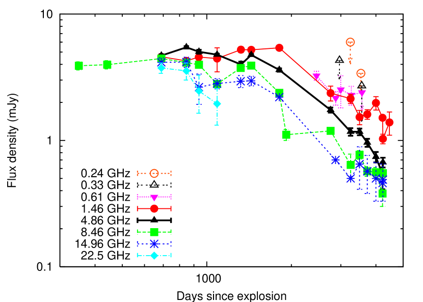
Figure 1: Light curves of SN 1995N in the 0.24 GHz, 0.33 GHz, 0.61 GHz, 1.46 GHz, 4.86 GHz, 8.46 GHz, 14.96 GHz and 22.50 GHz bands.

The details of each observation and the SN 1995N flux densities at various epochs are tabulated in Table 2. In Fig. 1 we plot the full dataset at all frequencies.

3 Radio Absorption Process

The radio emission in a SN is from the shocked interaction shell and is non-thermal synchrotron in nature. In the simplest models, it can initially be absorbed either by the internal medium due to synchrotron self absorption (SSA) or by the external medium through free-free absorption (FFA), depending on the mass loss rate of the presupernova star, magnetic field in the shocked shells, density of the ejecta and the CS parameters. Unfortunately, a clear distinction between the two absorption processes lies in the optically thick part of the light curve or spectrum, where the data for SN 1995N are quite sparse. Therefore, before attempting detailed model fits, we try to extract information about both absorption processes from other wavebands.

We can relate the free-free optical depth of the external medium to the hydrogen Balmer line luminosity, which can be written as (Osterbrook, 1989)

$$L_{\rm H\beta}=4.2\times 10^{-26}\int_{R}^{\infty}n_{R}^{2}\left(\frac{r}{R}\right)^{-4}4\pi r^{2}\,dr.$$ (1)

Here, cgs units are used and we assume the electron temperature of the CSM to be 20,000 K, deduced by Fransson et al. (2002) using the optical narrow line emission for SN 1995N. The radius $R$ is the outer radius of the shock and $n_{R}$ is the CSM density at a distance $R$ from the explosion center. Fransson et al. (2002) estimate the SN H$\beta$ luminosity to be $5.3\times 10^{36}$ erg s^-1. Thus, Eq. (1) gives $n_{R}^{2}R^{3}=10^{61}$ cm^-3. The free-free optical depth for this medium is $\tau_{\rm FFA}=\int_{R}^{\infty}\kappa_{ff}n_{R}^{2}\left(\frac{r}{R}\right)^{-4}dr$. Substituting $n_{R}^{2}R^{3}=10^{61}$ erg s^-1, this becomes

$$\tau_{\rm FFA}^{\rm H\beta}=0.5\left(\frac{\nu}{5\,\rm GHz}\right)^{-2}\left(\frac{T}{2\times 10^{4}\rm K}\right)^{-3/2}\left(\frac{R}{10^{17}\,\rm cm}\right)^{-2}.$$ (2)

Here $\tau_{\rm FFA}^{\rm H\beta}$ implies FFA optical depth derived from H$\beta$ luminosity. This exercise demonstrates that the optical depth derived from the H$\beta$ luminosity in the visual band reaches order unity at radio wavelengths, indicating that the FFA optical depth is sufficient to explain the radio absorption.

Chevalier & Fransson (2003, Fig. 7) plot the peak radio luminosity vs the time of peak radio flux for various supernovae, marking the lines of constant shock velocity derived assuming SSA absorption process. If we place SN 1995N in this plot, it falls close to a velocity of 3000 km s^-1. However, the optical line emission observations suggest ejecta velocities of at least 5000 km s^-1 (Fransson et al., 2002). Hence, the velocity of the radio-emitting region must be at least be equal to or greater than 5,000 km s^-1, an indication that SSA is not a significant factor in the the radio emission measured from SN 1995N. The H$\beta$ luminosity and the inferred expansion of the radio-emitting region suggest that FFA is the dominant radio absorption mechanism.

We now fit the FFA model to the data. The model for FFA was given by Chevalier (1982) and was formulated in detail by Van Dyk et al. (1994) and Weiler et al. (2002). The radio flux density, $F(\nu,t)$, under the FFA assumption can be written as:

$$F(\nu,t)=A_{1}\left(\frac{\nu}{5\,{\rm GHz}}\right)^{-\alpha}\left(\frac{t}{1000\,{\rm day}}\right)^{-\beta}\exp(-\tau_{\rm FFA})$$

$$\tau_{\rm FFA}=A_{2}\left(\frac{\nu}{5\,{\rm GHz}}\right)^{-2.1}\left(\frac{t}{1000\,{\rm day}}\right)^{-\delta},$$ (3)

where $\alpha$ is the frequency spectral index, which relates to electron energy index $\gamma$ ($N(E)\propto E^{-\gamma}$) as $\gamma=2\alpha+1$. To determine the value of $\alpha$, we plot spectral indices between 8.46 GHz and 4.86 GHz bands ($\alpha[8.46/4.86]$) as well as between 4.86 GHz and 1.46 GHz bands ($\alpha[4.86/1.46]$) at various epochs (see Fig 2). From Fig. 1, it is evident that the light curves becomes optically thin for these three bands after day $\sim 2500$. Thus we average both $\alpha(4.86/1.46)$ and $\alpha(8.46/4.86)$ for all the values after day 2500. The average spectral index is $\alpha=0.59\pm 0.07$. Hence, we use $\alpha=0.6$ ($\gamma=2.2$) in the radio absorption models. Here $A_{1}$ is the radio flux density normalization parameter and $A_{2}$ is the FFA optical depth normalization parameter. The parameter $\delta$ is related to the expansion parameter $m$ in $R\propto t^{m}$ as $\delta=3m$. The assumption that the energy density in the particles and the fields is proportional to the postshock energy density leads to $\beta=(\gamma+5-6m)/2$ (Chevalier, 1982). For $\gamma=2.2$, this becomes $\beta=3.6-3m$. Using these values, we fit the SN 1995N radio data to Eq. 3. The parameters for the best fit model are: $A_{1}=4.59\pm 0.19$, $A_{2}=(4.58\pm 0.80)\times 10^{-2}$, and $m=0.84\pm 0.02$. The above fit parameters yield $\delta=2.54\pm 0.06$, and $\beta=1.09\pm 0.06$. In the CS interaction model of Chevalier (1982), the power law index of the supernova density profile, $n$, is related to $m$ by $m=(n-3)/(n-2)$, so that the above value of $m$ implies $n=8.3$.

Although our fits for the FFA model are reasonable, we try to fit other radio absorption models as well. We use the formulation of Chevalier (1998) for the radio flux density with SSA present:

$$F(\nu,t)=P_{1}\left(\frac{t}{1000\,{\rm day}}\right)^{a}\left(\frac{\nu}{5\,{\rm GHz}}\right)^{5/2}\left(1-\exp(-\tau_{\rm SSA})\right),$$

$$\tau_{\rm SSA}=P_{2}\left(\frac{t}{1000\,{\rm day}}\right)^{-(a+b)}\left(\frac{\nu}{5\,{\rm GHz}}\right)^{-(\gamma+4)/2}.$$ (4)

Here $a$ gives the time evolution of the radio flux density in the optically thick phase ($F\propto t^{a}$) and $b$ in the optically thin phase ($F\propto t^{-b}$). Under the assumption that the energy density in the particles and the fields is proportional to the postshock energy density, these quantities are related with expansion parameter $m$ and electron energy index $\gamma$ as $a=2m+0.5$, and $b=(\gamma+5-6m)/2$ (as before). The estimation of $b$ from the fits is expected to be robust because there are ample data points in the optically thin part of the light curve, whereas $a$ is determined by the optically thick regime and cannot be constrained well due to sparse data in this region. Here $P_{1}$ is the flux normalization parameter and $P_{2}$ is the SSA optical depth normalization parameter. The best fit model gives $a=5.97\pm 1.13$ and $b=1.12\pm 0.07$. For $\gamma=2.2$, the above value of $b$ corresponds to $m=0.83$. The best fit value of $a$ corresponds to $m\gg 1$. However, $a$ is not well constrained by the data, so we fix it to a value of $a=2.16$, corresponding to $m=0.83$ and fit the data again. The best fits in this case are: $P_{1}=148.81\pm 34.77$, $P_{2}=(2.85\pm 0.68)\times 10^{-2}$, and $b=1.12\pm 0.06$. As expected, the evolution deduced during the optically thin case is similar to that found in the FFA model.

We note that there are more complicated possibilities for the absorption, but our data are not sufficient to test them. In particular, Weiler et al. (1990) found that the optically thick radio evolution of the Type IIn SN 1986J could not be fit by a model with external FFA, but could be fit by a model with internal FFA mixed with the synchrotron emitting region. Such a model is plausible for SNe IIn, because of the evidence for clumping in the CS medium, but we cannot test it here.

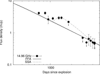
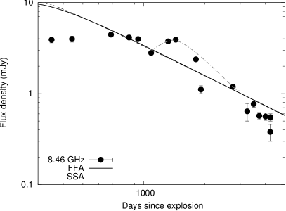
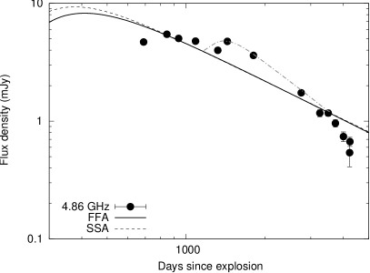
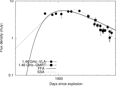
Figure 3: Light curves of SN 1995N in the 2 cm, 3.6 cm, 6 cm and 1.46 cm bands. The FFA absorption model is shown in solid lines and dashed lines represent the SSA absorption model. There are hints of bumps in the light curves soon after day 1200 in all the frequency bands (dashed-dotted lines), which may be due to the density clumps in the CSM.

Although both FFA and SSA give acceptable fits due to the lack of data points in the optically thick regime, the SSA derived velocity and information using optical data suggest that FFA is the most relevant radio absorption process. We produce light curves (see Fig. 3) and spectra (see Fig. 4) for both FFA and SSA processes. In Fig. 3, there is a sudden rise in the radio flux around day $\sim 1200$, plotted with grey dashed-dotted lines; this is evident in all the frequency bands almost at the same time. This effect can also be see in the spectra on days 1440 and 1812 (Fig. 4). We speculate that this feature is due to a density enhancement in the CSM. However, if the time decay $\beta$ is somewhat shallower at the early epoch, and there is a steepening in $\beta$ at later epochs, this may also cause such a bump in the light curves. Such time evolution in $\beta$ has been seen for SN 1993J and a few other supernovae (Weiler et al., 2007). It is difficult to distinguish between the two possibilities in view of the sparse data.

4 Physical Conditions

SN 1995N was extensively observed in many wavebands of the electromagnetic spectrum. We will utilize this information and derive constraints on various physical parameters of SN 1995N.

4.1 Mass loss rate

If FFA is the dominant absorption process, we can estimate the mass-loss rate of the progenitor star before it underwent the explosion phase using the radio data. This can be written as (Weiler et al., 1986; Van Dyk et al., 1994)

$$\dot{M}=2.11\times 10^{-5}\left[\frac{A_{2}}{10^{-2}}\right]^{0.5}\left[\frac{V_{ej}}{5,000\,{\rm km/s}}\right]^{1.5}\left[\frac{T_{e}}{20,000\,{\rm K}}\right]^{0.68}\left[\frac{u_{w}}{10\,{\rm km/s}}\right]\left[\frac{t}{1000\,{\rm day}}\right]^{3(1-m)/2}{\rm M_{\odot}\,yr^{-1}},$$ (5)

where $V_{ej}$ is the ejecta velocity and $T_{e}$ is the electron temperature. $A_{2}$ is the best fit normalization constant in the FFA model (see Eq. 3). The normalization values of $V_{ej}$ and $T_{e}$ are relevant for late time observations, say around the epoch of Chandra observations on day $\sim 3550$ (see §4.2). Assuming $u_{w}\approx 10$ km s^-1 gives a mass loss rate of $\dot{M}=(6.14\pm 0.47)\times 10^{-5}$ ${\rm M_{\odot}\,yr^{-1}}$; the error in mass loss rate is obtained using the best fit error in $A_{2}$. Uncertainties in the ejecta velocity, electron temperature and wind velocity introduce more uncertainty in the mass loss rate estimation. In addition, equation (5) is based on the assumption that the absorbing wind gas is smoothly distributed. However, Fransson et al. (2002) found that the density of ionized gas obtained from line diagnostics is higher than would be expected for smoothly distributed gas. With clumping, there is less matter for the same amount of absorption and the mass loss rate is reduced.

4.2 Density and temperature

SN 1995N was observed with XMM-Newton in July 2003 (Zampieri et al., 2005) and with Chandra in March 2004 (Chandra et al., 2005). We can use this information to extract the density structure of the SN ejecta around this time. It was estimated in Chandra et al. (2005) and Zampieri et al. (2005) that the total X-ray emission for SN 1995N around the time of the XMM and Chandra observations is $L_{X}=1.1\times 10^{40}$ erg s^-1. Chandra et al. (2005) estimated that most of the X-rays are coming from the reverse shock, and that there is a cooled shell present at the boundary of the reverse and forward shock with a column density of the cooling shell to be $N_{cool}=(9.1\pm 6.2)\times 10^{20}$ cm^-2. In the case of cooling, the total luminosity from the reverse shock can be written as (Chevalier & Fransson, 2003)

$$L_{rev}=2\times 10^{40}\,\frac{(n-3)(n-4)}{(n-2)^{3}}\left[\frac{\dot{M}}{10^{-5}{\rm\,M_{\odot}\,yr^{-1}}}\right]\left[\frac{u_{w}}{10\,{\rm km\,s^{-1}}}\right]^{-1}\left[\frac{V_{ej}}{5,000\,{\rm km\,s^{-1}}}\right]^{3}\,{\rm erg\,s^{-1}},$$ (6)

where $n$ is the power law density index of the SN ejecta ($\rho_{ej}\propto r^{-n}$, $\rho_{ej}$ ejecta density of the SN). Using the mass loss rate values derived in the above section (§4.1), Eq. 6 gives the ejecta density index $n\approx 8.5$. This value of $n$ is consistent with the one obtained from the radio evolution described in §3.

We can write the expression for the column density of the cooled shell in terms of mass loss rate as (Chevalier & Fransson, 2003)

$$N_{cool}=2\times 10^{20}\,(n-4)\left[\frac{\dot{M}}{10^{-5}{\rm M_{\odot}\,yr^{-1}}}\right]\left[\frac{u_{w}}{10\,{\rm km\,s^{-1}}}\right]^{-1}\left[\frac{V_{ej}}{5,000\,{\rm km\,s^{-1}}}\right]^{-1}\left[\frac{t}{1000\,{\rm days}}\right]^{-1}\,{\rm cm^{-2}}.$$ (7)

At the epoch of the Chandra observation, this gives $N_{cool}\approx 1.5\times 10^{21}$ cm^-2, which is in agreement with the value deduced from the X-ray observations ($(9.1\pm 6.2)\times 10^{20}$ cm^-2, Chandra et al., 2005).

Having an estimate for the mass loss rate and the density profile index, one can estimate the temperatures in the shocked circumstellar shell and the reverse shocked shell. The temperature of the shocked CSM shell is (Chevalier & Fransson, 2003)

$$T_{CS}=3.4\times 10^{8}\frac{(n-3)^{2}}{(n-2)^{2}}\left[\frac{{V_{ej}}}{5,000\,{\rm km\,s^{-1}}}\right]^{2}\,{\rm K}$$ (8)

and the reverse shock temperature is

$$T_{rev}=\frac{T_{CS}}{(n-3)^{2}}\,\rm K$$ (9)

The above equations give $T_{CS}=2.4\times 10^{8}$ K and $T_{rev}=0.9\times 10^{7}$ K. These estimates are derived assuming cosmic abundances and equipartition between ions and electrons. The equipartition time scale between electrons and ions is $t_{eq}\approx 290(T_{e}/10^{9}\,\rm K)^{1.5}(n_{e}/10^{7}\rm cm^{-3})^{-1}$ days. Chandra et al. (2005) estimate the electron density of the reverse shocked shell to be $n_{rev}\approx 2\times 10^{6}$ cm^-3. The density of the shocked CSM shell is thus $n_{cs}=2n_{rev}/(n-4)(n-3)=3.3\times 10^{5}$ cm^-3. This gives the estimates for equipartition time scales in the reverse shocked and the forward shocked shells as $1.3$ days and 1007.5 days, respectively. Hence, at the time of Chandra and XMM observations, the epoch at which the above parameters are derived, both the shocked shells have most likely attained electron-ion equilibrium.

5 Discussion and Conclusions

A useful way to characterize the radio emission from supernovae is by considering their peak radio luminosity and time of the peak; the more luminous Type II supernovae peak at a later time, indicating that they have a denser circumstellar medium (Chevalier, 2006). In such a plot, SN 1995N is close to the Type IIL SN 1979C and Type IIn SN 1978K, but is less luminous that the Type IIn SNe 1986J and 1988Z (Weiler et al., 1990; Williams et al., 2002). However, it is more radio luminous than many of the SNe IIn observed by Van Dyk et al. (1996).

The optically thin radio evolution of SN 1995N is fairly well defined and yields a radio spectral index $\alpha\approx 0.6$. This value is in the range found for Type II SNe and is smaller than the values found for Type Ib/c SNe (Weiler et al., 2002). The rate of decline is also similar to that found for other SNe II and, in a simple model for the emission, indicates an expansion factor for the emitting region $m=0.83$. Assuming interaction with a steady wind, the implied value of the power law index of the outer supernova density profile is $n\approx 8$. The same value of $n$ is consistent with the X-ray properties of SN 1995N.

Although there are clear indications of early low frequency absorption in the radio light curves of SN 1995N, there is little information on the evolution during the optically thick phase so that the nature of the absorption cannot be deduced from the radio light curves. Based on the emission measure of the gas deduced from optical observations and the late peak radio luminosity, we infer that free-free absorption is the likely absorption mechanism. The implied mass loss rate for the supernova progenitor is $6\times 10^{-5}\,{\rm M_{\odot}\,yr^{-1}}$, but this value has a number of uncertainties. The assumed velocity of the radio emitting region is $5000$ km s^-1; however, there are some indications from the H$\alpha$ line that there are higher velocities (Fransson et al., 2002), which would lead to a higher value of $\dot{M}$. The assumed wind velocity of 10 km s^-1 is lower than has been inferred from the narrow H$\alpha$ lines observed in some SNe IIn, e.g., 90 km s^-1 in SN 1997ab (Salamanca et al., 1998), 160 km s^-1 in SN 1997eg (Salamanca et al., 2002), and 100 km s^-1 in SN 2002ic (Kotak et al., 2004). An order of magnitude increase in $u_{w}$ would increase $\dot{M}$ by an order of magnitude. Finally, the optical line emission suggests clumping of the ionized wind gas (Fransson et al., 2002), which would reduce the estimate of $\dot{M}$ found here.

Regardless of the uncertainty in $\dot{M}$, the values deduced for SNe IIn from optical observations listed in § 1 are significantly larger than the value deduced for SN 1995N. In some of those cases, the mass loss may be a short lived event before the supernova. The long time coverage of SN 1995N, especially at radio wavelengths, shows that the circumstellar gas is extended in this case, out to radii $\gtrsim 2\times 10^{17}$ cm. The Type IIn supernovae are a heterogeneous group of objects.

Table 1: Details of phase calibration observations for SN 1995N

Date of	Telescope	Array	Frequency	Phase	Phase cal
observation		config.	in GHz	calibrator	Flux (Jy)
1995 Jun 16.19	VLA	DnA	8.46	1507-168	2.31
1995 Sep 15.96	VLA	BnA	8.46	1507-168	2.30
1996 May 21.20	VLA	CnD	4.86	1507-168	2.25
1996 May 21.20	VLA	CnD	8.46	1507-168	1.95
1996 May 21.24	VLA	CnD	1.46	1507-168	2.83
1996 May 21.24	VLA	CnD	14.96	1507-168	1.75
1996 May 21.25	VLA	CnD	22.48	1507-168	1.59
1996 Oct 24.71	VLA	A	1.46	1504-166	2.52
1996 Oct 24.72	VLA	A	8.46	1504-166	2.12
1996 Oct 24.73	VLA	A	4.86	1504-166	2.32
1996 Oct 24.76	VLA	A	22.48	1504-166	2.40
1996 Oct 24.76	VLA	A	14.96	1504-166	2.27
1997 Jan 23.61	VLA	BnA	1.46	1504-166	2.46
1997 Jan 23.62	VLA	BnA	8.46	1504-166	2.21
1997 Jan 23.63	VLA	BnA	4.86	1504-166	2.38
1997 Jan 23.64	VLA	BnA	14.96	1504-166	2.26
1997 Jan 23.64	VLA	BnA	22.48	1504-166	2.30
1997 Jun 22.99	VLA	BnC	1.46	1504-166	2.71
1997 Jun 23.00	VLA	BnC	8.46	1504-166	2.11
1997 Jun 23.02	VLA	BnC	4.86	1504-166	2.33
1997 Jun 23.03	VLA	BnC	14.96	1504-166	2.18
1997 Jun 23.04	VLA	BnC	22.48	1504-166	2.04
1998 Feb 10.00	VLA	DnA	14.96	1504-166	2.91
1998 Feb 10.00	VLA	DnA	8.46	1504-166	2.61
1998 Feb 13.37	VLA	DnA	1.46	1504-166	2.68
1998 Feb 13.49	VLA	DnA	4.86	1504-166	2.57
1998 Jun 10.14	VLA	BnA	0.33	1504-166	1.63
1998 Jun 10.16	VLA	BnA	1.46	1504-166	3.07
1998 Jun 10.17	VLA	BnA	8.46	1504-166	3.13
1998 Jun 10.19	VLA	BnA	14.96	1504-166	3.84
1998 Jun 10.20	VLA	BnA	4.86	1504-166	2.80
1999 Jun 17.23	VLA	DnA	1.46	1504-166	2.77
1999 Jun 17.25	VLA	DnA	4.86	1504-166	2.78
1999 Jun 17.26	VLA	DnA	8.46	1504-166	2.68
1999 Jun 17.27	VLA	DnA	14.96	1504-166	2.90
1999 Oct 01.89	VLA	BnA	8.46	1504-166	2.82
2000 Nov 08.00	GMRT	$-$	1.42	1347+122	6.25
2001 Mar 25.00	GMRT	$-$	0.61	1419+064	16.07
2002 Jan 19.65	VLA	D	1.46	1504-166	2.94
2002 Jan 19.67	VLA	D	4.86	1504-166	2.54
2002 Jan 19.67	VLA	D	8.46	1504-166	2.13
2002 Apr 07.00	GMRT	$-$	1.41	1445+099	2.40
2002 May 15.24	VLA	A	14.96	1504-166	1.70
2002 May 19.00	GMRT	$-$	0.61	1419+064	16.17
2002 Aug 16.00	GMRT	$-$	0.33	1419+064	29.65
2002 Sep 16.00	GMRT	$-$	0.61	1419+064	16.17
2002 Sep 21.00	GMRT	$-$	1.41	1351-148	1.12
2003 May 26.30	VLA	A	1.46	1504-166	2.99
2003 May 26.31	VLA	A	4.86	1504-166	2.34
2003 May 28.22	VLA	A	8.46	1504-166	2.03
2003 May 28.24	VLA	A	14.96	1504-166	1.64
2003 Jun 13.00	GMRT	$-$	1.30	1432-180	0.81
2003 Jun 16.00	GMRT	$-$	0.61	1419+064	15.18
2003 Jun 16.00	GMRT	$-$	0.24	1419+064	44.58
2004 Jan 29.48	VLA	BnC	1.46	1504-166	2.99
2004 Jan 29.50	VLA	BnC	4.86	1504-166	2.37
2004 Jan 29.51	VLA	BnC	14.96	1504-166	1.71
2004 Jan 29.52	VLA	BnC	8.46	1504-166	2.05
2004 Feb 13.00	GMRT	$-$	1.30	1432-180	1.01
2004 Mar 29.00	GMRT	$-$	1.30	1432-180	1.00
2004 Apr 01.00	GMRT	$-$	0.33	1419+064	26.57
2004 Apr 08.00	GMRT	$-$	0.61	1419+064	19.71
2004 Apr 08.00	GMRT	$-$	0.24	1419+064	40.96
2004 Sep 06.99	VLA	A	22.460	1512-090	4.96
2004 Sep 12.94	VLA	A	1.46	1507-168	2.86
2004 Sep 12.95	VLA	A	4.86	1507-168	2.52
2004 Sep 12.96	VLA	A	8.46	1507-168	1.97
2004 Sep 12.97	VLA	A	14.96	1507-168	1.66
2005 Jun 14.30	VLA	BnC	1.46	1507-168	2.93
2005 Jun 14.31	VLA	BnC	4.86	1507-168	2.40
2005 Jun 14.32	VLA	BnC	8.46	1507-168	2.09
2005 Jun 14.33	VLA	BnC	14.96	1507-168	1.75
2006 Jan 23.60	VLA	D	1.46	1507-168	2.77
2006 Jan 23.61	VLA	D	4.86	1507-168	2.24
2006 Jan 23.63	VLA	D	8.46	1507-168	1.87
2006 Jan 23.65	VLA	D	14.96	1507-168	1.53
2006 Feb 02.59	VLA	A	4.86	1507-168	2.16
2006 Feb 02.60	VLA	A	1.46	1507-168	2.27
2006 Feb 02.62	VLA	A	8.46	1507-168	1.91
2006 Feb 02.63	VLA	A	14.96	1507-168	0.77
2006 Sep 26.00	VLA	BnC	8.46	1507-168	1.75
2006 Sep 26.00	VLA	BnC	1.46	1507-168	2.62
2006 Sep 26.01	VLA	BnC	4.86	1507-168	2.42

Table 2: Radio observations of the SN 1995N

Date of	Days since	Telescope	Array	Frequency	RMS	Flux density
observation	explosion		config.	in GHz	$\mu$Jy	mJy
1995 Jun 16.19	350.19	VLA	DnA	8.46	210	$3.90\pm 0.29$
1995 Sep 15.96	441.96	VLA	BnA	8.46	220	$3.98\pm 0.30$
1996 May 21.20	688.76	VLA	CnD	4.86	66	$4.69\pm 0.12$
1996 May 21.20	688.76	VLA	CnD	8.46	58	$4.45\pm 0.09$
1996 May 21.24	688.80	VLA	CnD	1.46	167	$4.37\pm 0.77$
1996 May 21.24	689.02	VLA	CnD	14.96	186	$4.15\pm 0.35$
1996 May 21.25	689.03	VLA	CnD	22.48	249	$3.75\pm 0.35$
1996 Oct 24.71	845.52	VLA	A	1.46	106	$4.26\pm 0.19$
1996 Oct 24.72	845.53	VLA	A	8.46	75	$4.13\pm 0.12$
1996 Oct 24.73	845.54	VLA	A	4.86	66	$5.46\pm 0.12$
1996 Oct 24.76	845.57	VLA	A	22.48	328	$3.55\pm 0.55$
1996 Oct 24.76	845.57	VLA	A	14.96	208	$4.17\pm 0.39$
1997 Jan 23.61	936.42	VLA	BnA	1.46	178	$4.57\pm 0.30$
1997 Jan 23.62	937.43	VLA	BnA	8.46	94	$3.74\pm 0.16$
1997 Jan 23.63	937.44	VLA	BnA	4.86	105	$5.03\pm 0.18$
1997 Jan 23.64	937.45	VLA	BnA	14.96	408	$2.64\pm 0.71$
1997 Jan 23.64	937.45	VLA	BnA	22.48	622	$2.46\pm 0.82$
1997 Jun 22.99	1087.80	VLA	BnC	1.46	170	$4.45\pm 0.96$
1997 Jun 23.00	1087.81	VLA	BnC	8.46	81	$2.80\pm 0.04$
1997 Jun 23.02	1087.83	VLA	BnC	4.86	55	$4.77\pm 0.09$
1997 Jun 23.03	1087.84	VLA	BnC	14.96	155	$2.82\pm 0.26$
1997 Jun 23.04	1087.85	VLA	BnC	22.48	320	$1.95\pm 0.63$
1998 Feb 10.00	1320.00	VLA	DnA	14.96	233	$2.94\pm 0.32$
1998 Feb 10.00	1320.00	VLA	DnA	8.46	37	$3.75\pm 0.13$
1998 Feb 13.37	1323.22	VLA	DnA	1.46	82	$5.23\pm 0.27$
1998 Feb 13.49	1323.35	VLA	DnA	4.86	71	$3.99\pm 0.21$
1998 Jun 10.14	1439.99	VLA	BnA	0.33	12504	$<25.00$
1998 Jun 10.16	1440.01	VLA	BnA	1.46	101	$5.21\pm 0.17$
1998 Jun 10.17	1440.03	VLA	BnA	8.46	41	$3.91\pm 0.07$
1998 Jun 10.19	1440.04	VLA	BnA	14.96	160	$2.96\pm 0.26$
1998 Jun 10.20	1440.05	VLA	BnA	4.86	44	$4.75\pm 0.08$
1999 Jun 17.23	1812.08	VLA	DnA	1.46	58	$5.41\pm 0.12$
1999 Jun 17.25	1812.10	VLA	DnA	4.86	66	$3.61\pm 0.11$
1999 Jun 17.26	1812.11	VLA	DnA	8.46	60	$2.58\pm 0.10$
1999 Jun 17.27	1812.12	VLA	DnA	14.96	195	$<2.2$
1999 Oct 01.89	1918.74	VLA	BnA	8.46	46	$1.11\pm 0.11$
2000 Nov 08.00	2320.85	GMRT	$-$	1.42	290	$3.87\pm 0.50$
2001 Mar 25.00	2457.85	GMRT	$-$	0.61	130	$3.26\pm 0.27$
2002 Jan 19.65	2758.51	VLA	D	1.46	91	$2.37\pm 0.32$
2002 Jan 19.67	2758.53	VLA	D	4.86	46	$1.74\pm 0.08$
2002 Jan 19.67	2758.53	VLA	D	8.46	39	$1.19\pm 0.07$
2002 Apr 07.00	2835.86	GMRT	$-$	1.41	310	$3.05\pm 0.52$
2002 May 15.24	2874.09	VLA	A	14.96	232	$<0.70$
2002 May 19.00	2877.86	GMRT	$-$	0.61	130	$2.17\pm 0.27$
2002 Aug 16.00	2966.86	GMRT	$-$	0.33	780	$<4.30$
2002 Sep 16.00	2997.86	GMRT	$-$	0.61	390	$2.53\pm 0.72$
2002 Sep 21.00	3002.86	GMRT	$-$	1.41	100	$2.21\pm 0.30$
2003 May 26.30	3250.15	VLA	A	1.46	97	$2.14\pm 0.18$
2003 May 26.31	3250.16	VLA	A	4.86	51	$1.17\pm 0.08$
2003 May 28.22	3252.09	VLA	A	8.46	44	$0.64\pm 0.14$
2003 May 28.24	3252.11	VLA	A	14.96	166	$<0.50$
2003 Jun 13.00	3267.87	GMRT	$-$	1.30	380	$1.66\pm 0.47$
2003 Jun 16.00	3270.87	GMRT	$-$	0.61	190	$2.29\pm 0.39$
2003 Jun 16.00	3270.87	GMRT	$-$	0.24	3030	$<5.00$
2004 Jan 29.48	3498.23	VLA	BnC	1.46	115	$1.53\pm 0.20$
2004 Jan 29.50	3498.25	VLA	BnC	4.86	43	$1.17\pm 0.07$
2004 Jan 29.51	3498.26	VLA	BnC	14.96	134	$0.65\pm 0.24$
2004 Jan 29.52	3498.27	VLA	BnC	8.46	36	$0.77\pm 0.06$
2004 Feb 13.00	3512.75	GMRT	$-$	1.30	210	$1.59\pm 0.23$
2004 Mar 29.00	3557.75	GMRT	$-$	1.30	140	$1.61\pm 0.28$
2004 Apr 01.00	3560.75	GMRT	$-$	0.33	840	$<2.4$
2004 Apr 08.00	3567.75	GMRT	$-$	0.61	140	$<2.42$
2004 Apr 08.00	3567.75	GMRT	$-$	0.24	1740	$<3.50$
2004 Sep 06.99	3720.99	VLA	A	22.460	187	$<0.50$
2004 Sep 12.94	3726.94	VLA	A	1.46	60	$1.61\pm 0.14$
2004 Sep 12.95	3726.95	VLA	A	4.86	52	$0.96\pm 0.07$
2004 Sep 12.96	3726.96	VLA	A	8.46	42	$0.57\pm 0.05$
2004 Sep 12.97	3726.97	VLA	A	14.96	189	$0.57\pm 0.19$
2005 Jun 14.30	4001.30	VLA	BnC	1.46	184	$1.98\pm 0.24$
2005 Jun 14.31	4001.31	VLA	BnC	4.86	56	$0.74\pm 0.07$
2005 Jun 14.32	4001.32	VLA	BnC	8.46	44	$0.56\pm 0.05$
2005 Jun 14.33	4001.33	VLA	BnC	14.96	166	$0.50\pm 0.17$
2006 Jan 23.60	4225.08	VLA	D	1.46	551	$<1.51$
2006 Jan 23.61	4225.09	VLA	D	4.86	80	$0.54\pm 0.13$
2006 Jan 23.63	4225.11	VLA	D	8.46	55	$0.38\pm 0.08$
2006 Jan 23.65	4225.13	VLA	D	14.96	152	$<0.46$
2006 Feb 02.59	4234.59	VLA	A	4.86	47	$0.67\pm 0.06$
2006 Feb 02.60	4234.60	VLA	A	1.46	52	$1.03\pm 0.09$
2006 Feb 02.62	4234.62	VLA	A	8.46	40	$0.55\pm 0.05$
2006 Feb 02.63	4234.63	VLA	A	14.96	164	$0.49\pm 0.16$
2006 Sep 26.00	4470.00	VLA	BnC	8.46	40	$<0.32$
2006 Sep 26.00	4470.00	VLA	BnC	1.46	190	$1.39\pm 0.29$
2006 Sep 26.01	4470.01	VLA	BnC	4.86	83	$0.25\pm 0.08$

Figure 2: Spectral index evolution between 8.46 GHz and 4.86 GHz (upper panel), and between 4.86 GHz and 1.46 GHz. The thick dashed line is plotted by averaging all the values of the spectral index after day 2500.

Figure 4: Near simultaneous spectra of SN 1995N on various days. FFA absorption is shown in solid lines and dashed lines represent the SSA absorption. Here filled circles represent VLA data and filled squares represent GMRT data. Please note that models do not fit the spectra well on days when bumps are seen in the light curves, i.e. around day 1200.

References

- Chandra et al. (2005) Chandra, P., Ray, A., Schlegel, E. M., Sutaria, F. K., & Pietsch, W. 2005, ApJ, 629, 933
- Chandra et al. (2005b) Chandra, P. 2005, Ph.D. thesis, Indian Institute of Science
- Chevalier (2006) Chevalier, R. A. 2006, ArXiv Astrophysics e-prints, arXiv:astro-ph/0607422