The transverse proximity effect in the $z\sim 2$ Lyman-$\alpha$ forest suggests QSO episodic lifetimes of $\sim 1$ Myr

Abstract

We look for signs of the H I transverse proximity effect in the spectra of 130 QSO pairs, most with transverse separations in the plane of the sky of 0.1 – 3 Mpc at $z\sim 2.2$. We expected to see a decrease in Ly$\alpha$ forest H I absorption in the spectrum of background QSOs near the position of foreground QSOs. Instead we see no change in the absorption in front of the foreground QSOs, and we see evidence for a 50% increase in the absorption out to 6 Mpc behind the foreground QSOs. Further, we see no change in the H I absorption along the line-of-sight to the foreground QSOs, the normal line-of-sight proximity effect. We may account for the lack of change in the H I absorption if the effect of extra UV photons is cancelled by higher gas density around QSOs. If so, the increase in absorption behind the QSOs then suggests that the higher gas density there is not cancelled by the UV radiation from the QSOs. We can explain our observations if QSOs have had their current UV luminosities for less than approximately a million years, a time scale that has been suggested for accretion disk instabilities and gas depletion.

1 Introduction

Quasars are the most luminous known objects in the universe at 1 Ryd, at least among objects that are luminous more than a few hours. Consequently, they are expected to have a profound effect on neutral hydrogen (H I) in the nearby intergalactic medium (IGM). This is because in most of the volume of the IGM the H I is expected to be optically thin and in photoionization equilibrium with the metagalactic UV background (UVB), so the enormous UV flux from the QSO will significantly alter the photoionization equilibrium and reduce the amount of neutral hydrogen. The UV flux from a typical QSO at $z=2$ should dominate the UVB as far away as 5 Mpc from the QSO. The resulting decrease in the optical depth of the Ly$\alpha$ forest at redshifts near to the systemic redshift of the QSO is known as the proximity effect.

We define two proximity effects: the line-of-sight proximity effect where the H I optical depth is measured in the spectrum of the QSO that is the source of the ionizing radiation, and the transverse proximity effect where the H I optical depth is measured in the spectrum of an object which is near to the QSO in the plane of the sky and further away. Some other groups call the transverse proximity effect the foreground proximity effect. The line-of-sight proximity effect is expected to be present in the spectra of all QSOs unless there is an intervening optically thick absorber or the episodic lifetime of the QSO is shorter than the inverse H I ionization rate in the IGM (0.1 Myr), i.e. the time required for each H I atom to experience one photoionization.

We use “episodic lifetime” in the same sense as Martini (2004), meaning the lifetime of the current outburst and not the integrated “on” time of the QSO. If QSOs have many episodes of high UV luminosity, separated by off states with low luminosity, the total QSO lifetime may be much longer than the duration of the current UV luminous episode (Martini, 2004). An episodic lifetime less than a few Myr will significantly change the appearance of the transverse proximity effect (Adelberger 2004, Fig. 3, Schirber et al. 2004, Visbal & Croft 2008, Fig. 1, and Tytler et al. 2008a, Fig. 24).

The purpose of this paper is to measure the transverse proximity effect in a large sample of QSO pairs that are separated in the plane of the sky by $<3$ Mpc. We also measure the line-of-sight proximity effect and compare it to the transverse effect because this helps us explore the environments of the QSOs, anisotropic emission and episodic lifetimes.

The line-of-sight proximity effect has been detected numerous times in the spectra of tens of the brightest QSOs known at redshifts 1.6 – 4. It was first seen by Carswell et al. (1982) and Tytler (1987) in the spectra of 7 and 19 QSOs, mostly at $z\sim 2$. They noticed a decrease in the number of Ly$\alpha$ lines at redshifts similar to QSO emission redshifts. Like most early papers, they used a sample of Ly$\alpha$ lines with rest frame equivalent widths exceeding a fixed minimum (0.32 Å) and they excluded lines at redshifts that show metal lines in moderate resolution spectra. The line-of-sight proximity effect can be seen in high resolution spectra of individual QSOs at high redshift (Carswell et al., 1987; Giallongo et al., 1996) where there is more Ly$\alpha$ absorption. If QSOs are located in typical regions of the IGM, then the amount of H I absorption that is missing and the distance from QSOs at which this occurs depends only upon the ratio of the flux of ionizing photons from the QSO to the UVB. Hence Bajtlik et al. (1988) were able to use the effect to estimate the intensity of the UVB in the Lyman continuum near the Lyman Limit, and others have improved upon this method (Scott et al., 2000).

Recently, Guimarães et al. (2007) used ESI spectra to examine the proximity effect of 45 $z>4$ QSOs. They found significantly more absorption than expected based upon the luminosity of the QSOs: they conclude that the QSOs must reside in regions were the IGM is over-dense by a factor of $\sim 5$. A similar result was previously reported by Rollinde et al. (2005).

We expect the gas near to QSOs to have higher than the average density in the IGM because QSOs are in galaxies and the halo masses are large. Croom et al. (2005) estimated QSO halo masses of $4.2\pm 2.3\times 10^{12}$ solar masses in the 2QZ sample at all redshifts. Coil et al. (2007) also found a mean mass of $\sim 3\times 10^{12}$ at $0.7<z<1.4$. Less directly, Kim & Croft (2008) use the distribution of H I absorption seen in background QSOs to estimate the masses of foreground QSO halos. They find a mean mass of $\log M=12.48^{+0.53}_{-0.89}$ in solar units for QSOs at $z=3$ with an absolute G-band magnitude $-27.5$, a factor of 20 above the mass of LBGs. We also expect the gas near QSOs to have higher density than the average IGM because Adelberger (2004, Fig 14) sees excess Ly$\alpha$ absorption within 1 Mpc proper of LBGs.

The idea that QSOs are found in relatively dense environments is also supported by the discovery that absorption is often produced when a sightline passes within 100 kpc of a QSO. Absorbers are more often seen in this case than when we look directly at a QSO. Bowen et al. (2006) discovered this effect with Mg II absorption in four out of four QSOs, while Hennawi et al. (2006) saw the same for Lyman limit systems (LLS) and Damped Ly$\alpha$ lines (DLAs), and we have also seen the effect in metal line systems with a super-set of the data examined here (Tytler et al., 2008a). Hennawi & Prochaska (2007) conclude that QSOs live in dense environments, and that the UV flux from the QSO photo-evaporates LLS along the line-of-sight. But because of either anisotropic emission or short QSO episodic lifetimes, some of the LLS in the transverse direction are spared or are less likely to be photo-evaporated. Wild et al. (2008) estimate that QSOs destroy nearby absorbers to comoving distances of 0.3 Mpc for C IV systems, and 0.8 Mpc for Mg II systems.

For ions other than Hydrogen, enhanced ionization near to a foreground QSO has been reported by several authors. Jakobsen et al. (2003) find a significant lack of HeII absorption in the spectrum of Q0302-003 at the redshift of a foreground QSO located $\sim 3$ Mpc from the Q0302-003 line-of-sight. Similarly, Worseck et al. (2007) examined both the HeII absorption and the H I absorption towards HE 2347-4342, and found evidence for a hard ionizing spectrum near the redshifts of 14 low luminosity foreground QSOs. Gonçalves et al. (2008) have also detected unusual high ionization absorption systems (e.g. O VI) indicative of a transverse proximity effect in high resolution spectra of the QSO triplet KP76, KP77, and KP78.

In contrast, an H I transverse proximity effect has yet to be detected, with perhaps one exception (Gallerani et al., 2008). It is interesting in part because Adelberger (2004) has pointed out that the transverse proximity effect is one of the best ways to explore changes in the UV luminosity over several Myr. Both Wang et al. (2005) and Visbal & Croft (2008) discuss how we may obtain similar information from afterglows or light-echoes from QSOs that were previously luminous.

Liske & Williger (2001) detected the line-of-sight proximity effect in a group of 10 QSOs near $z=2.9$ with transverse separations of 10–40′. But with the exception of the sightline that passes about 10′ from four separate foreground QSOs, they do not detect a transverse proximity effect. They conclude that QSOs emit at least a factor of 1.4 less in the plane of the sky than they do along the line-of-sight. Schirber et al. (2004) also did not detect the transverse proximity effect, using three pairs of SDSS spectra separated by $\sim$ 2 – 4′.

Croft (2004) analyzed a sample of 325 QSOs with SDSS spectra. He also failed to detect a transverse proximity, although his sample was less sensitive than ours because it had almost no QSO pairs as close as ours. Croft (2004) actually observed an increase in the mean absorption near to QSOs in the transverse direction, at a level much higher than expected by his simulations which placed QSOs in high density regions. This may be related to the Bowen et al. (2006), Hennawi et al. (2006) and Tytler et al. (2008a) results, since it is likely that the Croft (2004) simulations, like most simulations, underestimate the number of LLS and DLA systems (Tytler et al., 2008b). Recently Gallerani et al. (2008) have reported an increased density of flux spikes near a foreground QSO at z=5.6 that they model as the first example of the transverse H I proximity effect.

In this paper we look for the H I transverse proximity effect in a large sample of sightlines passing within 0.1 – 3 Mpc of QSOs. We do not see the obvious transverse proximity effect expected if the UV flux from QSOs is long lived and emitted isotropically. But we do detect asymmetry in the absorption around the QSOs, which may be a result of a combination of enhanced IGM density within a few Mpc of QSOs, combined with short episodic lifetimes for QSO outbursts. We can understand our observations if the QSOs were much less UV luminous $\sim$ 1 Myr ago than they are today. For all of the calculations in this paper we take $H_{0}=71$ km s^-1 Mpc^-1, $\Omega_{m}=0.27$, and $\Omega_{\Lambda}=0.73$. All distances in this paper are proper, unless noted otherwise.

2 Data

Table 1: QSO Pairs. For each member of the pair we give the RA and Dec (J2000), the adopted emission redshift $z_{\rm em}$, magnitude, and the SNR per Å (S) at 1260 Å in the QSO rest frame. The background QSO is listed first. $\theta$ is the angular separation on the sky between the 2 QSOs in arcseconds, and $b$ is the impact parameter in proper Mpc between the two sightlines at the $z_{\rm em}$ of the foreground QSO. $L$ is the estimated Lyman Limit luminosity in units of $10^{30}$ ergs s^-1 Hz^-1. $\omega_{\rm max}$ is the expected ratio of the UV flux from the foreground QSO to the UVB, at the point of closest approach of the background sightline to the foreground QSO.

RA	Dec	$z_{\rm em}$	mag	S	RA	Dec	$z_{\rm em}$	mag	S	$\theta$	$b$	$L$	$\omega_{\rm max}$
11 16 10.7	$+$41 18 14.5	2.995	19.5 g	9	11 16 11.7	$+$41 18 21.5	2.983	18.6 g	19	13.7	0.10	13	2272.5
09 09 23.1	$+$00 02 03.9	1.893	20.2 g	36	09 09 24.0	$+$00 02 11.0	1.878	16.8 g	102	15.0	0.12	22	2715.3
03 13 25.5	$-$31 41 54.3	2.075	20.1 bJ	33	03 13 24.4	$-$31 41 44.9	1.965	20.0 bJ	31	17.0	0.14	1.3	123.1
02 18 21.4	$-$29 53 40.9	2.067	20.1 bJ	66	02 18 23.0	$-$29 53 31.3	1.919	19.2 bJ	77	22.0	0.18	2.6	149.7
11 07 27.1	$+$00 34 07.3	1.890	20.2 g	29	11 07 25.7	$+$00 33 53.6	1.881	19.1 g	58	24.8	0.21	2.7	119.5
21 48 36.6	$-$29 40 54.2	2.098	20.1 bJ	102	21 48 34.9	$-$29 41 09.9	1.822	19.6 bJ	36	26.7	0.22	1.6	62.4
13 06 34.2	$+$29 24 43.1	1.978	19.1 V	30	13 06 35.4	$+$29 25 05.9	1.938	20.6 V	34	27.8	0.23	0.71	25.1
21 43 07.0	$-$44 50 47.6	3.270	21.3 V	25	21 43 04.1	$-$44 50 36.0	3.067	21.1 V	24	33.2	0.25	1.1	33.0
14 35 06.4	$+$00 09 01.5	2.389	20.0 bJ	4	14 35 08.3	$+$00 08 44.4	2.384	20.1 bJ	2	33.2	0.27	2	53.8
23 53 13.0	$-$27 26 09.4	2.308	20.1 bJ	10	23 53 10.0	$-$27 26 14.1	1.963	18.7 bJ	52	40.3	0.33	4.4	74.1
23 59 45.5	$-$00 58 19.6	1.820	18.7 g	77	23 59 44.1	$-$00 57 38.2	1.795	19.5 g	48	46.2	0.38	1.7	21.2
23 09 11.9	$-$27 32 27.1	1.932	19.4 bJ	30	23 09 15.3	$-$27 32 45.3	1.927	20.2 bJ	4	49.5	0.41	1.1	12.3
22 32 20.3	$-$28 38 58.7	2.207	19.9 bJ	7	22 32 23.4	$-$28 38 29.9	2.073	20.3 bJ	36	50.8	0.42	1.1	12.2
03 06 43.7	$-$30 11 07.5	2.127	19.8 bJ	18	03 06 40.9	$-$30 10 31.9	2.099	19.3 bJ	35	51.2	0.42	2.9	30.6
02 56 42.6	$-$33 15 21.0	1.915	17.0 V	35	02 56 47.0	$-$33 15 27.0	1.872	16.5 V	19	55.8	0.46	29	251.2
09 27 47.3	$+$29 07 20.7	2.304	18.6 g	13	09 27 43.0	$+$29 07 34.7	2.254	19.1 g	9	57.4	0.47	3.8	33.2
03 10 06.1	$-$19 21 24.9	2.152	18.6 V	74	03 10 09.0	$-$19 22 08.1	2.129	19.1 V	37	60.3	0.49	3.3	25.3
21 42 25.9	$-$44 20 17.0	3.242	18.7 V	12	21 42 22.2	$-$44 19 30.0	3.227	21.2 V	59	61.5	0.46	1.1	10.0
22 39 51.8	$-$29 48 37.0	2.130	18.8 bJ	81	22 39 48.6	$-$29 47 48.7	2.071	20.2 bJ	32	63.6	0.52	1.2	8.6
08 15 18.3	$+$06 06 04.3	2.536	20.2 g	7	08 15 14.3	$+$06 05 42.5	2.505	20.4 g	4	64.1	0.51	1.6	11.5
09 14 10.3	$+$46 10 50.0	2.358	20.2 V	5	09 14 04.1	$+$46 10 44.9	2.191	21.0 V	2	64.6	0.53	0.57	3.9
10 41 29.3	$+$56 30 23.0	2.267	19.0 g	11	10 41 21.9	$+$56 30 01.0	2.051	18.3 g	16	65.1	0.54	6.7	44.3
23 01 17.6	$-$31 43 59.2	2.140	19.1 bJ	65	23 01 12.4	$-$31 43 45.0	1.991	19.7 bJ	36	67.8	0.56	1.8	10.8
10 16 05.8	$+$40 40 05.8	2.995	20.5 g	4	10 16 01.5	$+$40 40 52.9	2.984	19.6 g	8	68.2	0.52	5.3	36.7
03 10 36.5	$-$30 51 08.4	2.566	20.4 bJ	13	03 10 41.1	$-$30 50 27.5	2.546	19.5 bJ	22	71.9	0.57	4.1	23.8
14 57 56.3	$+$57 44 46.9	2.125	19.7 g	7	14 57 47.5	$+$57 44 23.5	2.014	19.3 g	9	73.6	0.61	2.6	13.2
12 12 51.1	$-$00 53 42.2	2.480	20.4 bJ	1	12 12 56.1	$-$00 53 36.5	2.467	20.8 bJ	2	74.0	0.59	1.2	6.4
00 08 52.7	$-$29 00 44.1	2.656	19.1 bJ	133	00 08 57.7	$-$29 01 26.9	2.615	19.8 bJ	89	78.5	0.62	3.4	16.5
00 45 27.5	$-$32 01 35.4	2.006	19.8 bJ	45	00 45 26.5	$-$32 00 16.9	1.896	19.0 bJ	68	79.6	0.66	3.2	13.8
01 02 57.4	$-$27 53 38.8	1.820	19.3 bJ	36	01 02 51.9	$-$27 53 03.3	1.801	18.2 V	51	81.1	0.67	5.5	23.0
00 44 34.1	$+$00 19 03.5	1.878	19.2 g	21	00 44 39.3	$+$00 18 22.8	1.875	18.3 g	30	88.6	0.73	5.6	19.4
15 45 34.6	$+$51 12 28.0	2.458	19.5 g	4	15 45 44.2	$+$51 13 07.0	2.252	19.3 g	6	98.3	0.80	3.2	9.4
01 24 53.1	$-$28 52 51.5	2.100	18.8 bJ	78	01 24 56.4	$-$28 51 21.0	1.998	19.0 bJ	54	100.7	0.83	3.3	9.0
15 19 19.4	$+$23 46 02.0	1.907	16.4 V	54	15 19 13.3	$+$23 46 58.7	1.846	18.4 V	26	101.3	0.84	4.8	12.7
17 36 35.5	$+$55 28 29.4	1.997	19.9 g	39	17 36 26.7	$+$55 27 20.7	1.831	20.4 g	29	101.5	0.84	0.76	2.0
11 06 11.1	$+$13 56 00.0	3.912	21.5 g	6	11 06 16.7	$+$13 54 58.6	3.854	21.3 g	6	101.7	0.71	3.5	13.0
13 39 39.0	$+$00 10 22.0	2.124	19.3 g	57	13 39 45.4	$+$00 09 45.0	1.879	19.3 g	36	102.9	0.85	2.2	5.8
16 23 24.8	$+$33 10 49.8	2.593	18.1 g	21	16 23 23.7	$+$33 12 32.6	2.420	19.0 g	13	103.7	0.83	5	13.6
17 19 32.9	$+$29 19 29.0	3.303	20.3 g	5	17 19 37.9	$+$29 18 05.0	3.075	20.7 g	3	106.5	0.81	2.1	6.0
14 22 39.9	$+$42 02 20.4	3.228	19.5 g	9	14 22 49.2	$+$42 02 46.2	3.077	20.1 g	4	106.9	0.81	3.7	10.6
13 21 47.7	$+$01 06 04.8	2.138	20.1 g	54	13 21 54.3	$+$01 06 51.9	1.983	20.1 g	22	110.6	0.91	1.2	2.7
17 27 56.4	$+$58 21 55.7	2.373	19.3 g	49	17 28 06.8	$+$58 20 39.2	2.019	19.4 g	37	111.6	0.92	2.4	5.3
11 08 19.1	$-$00 58 24.0	4.567	23.5 g	7	11 08 13.9	$-$00 59 44.5	4.027	21.0 g	11	113.0	0.78	5.3	16.6
11 52 00.5	$+$45 17 41.4	2.406	19.2 g	10	11 52 10.4	$+$45 18 25.8	2.311	19.1 g	9	113.4	0.92	4	8.9
16 12 45.6	$+$23 58 00.0	2.040	19.6 g	22	16 12 37.9	$+$23 57 09.0	2.018	19.4 V	19	117.2	0.97	2.3	4.7
15 09 32.2	$+$50 57 51.5	2.377	18.8 g	11	15 09 25.6	$+$50 56 09.3	2.375	19.0 g	12	119.7	0.96	4.7	9.4
13 46 21.4	$-$00 38 05.0	1.895	20.1 bJ	12	13 46 25.6	$-$00 39 47.0	1.851	19.3 bJ	10	119.9	0.99	2.2	4.1
02 09 54.8	$-$10 02 23.0	1.980	19.6 r	16	02 10 00.1	$-$10 03 54.0	1.979	19.3 g	51	120.0	0.99	2.5	4.8
15 08 38.1	$+$60 35 40.1	2.188	19.0 g	13	15 08 27.7	$+$60 34 07.4	1.901	18.1 g	20	120.5	1.00	6.9	13.0
10 05 41.3	$+$57 05 44.0	2.324	18.1 g	12	10 05 38.5	$+$57 07 44.0	1.874	18.9 g	4	122.1	1.01	3.2	5.9
00 55 57.5	$-$32 55 39.0	2.257	19.6 V	41	00 56 05.3	$-$32 56 51.1	2.134	19.6 V	5	122.5	1.00	2.1	3.9
10 19 22.9	$+$55 24 31.0	3.728	21.5 g	3	10 19 37.0	$+$55 23 55.0	3.236	20.5 g	4	125.4	0.93	3	6.5
15 48 50.2	$+$53 38 43.0	2.192	19.8 g	4	15 48 40.8	$+$53 37 08.6	2.172	18.8 g	10	126.1	1.03	4.8	8.4
11 04 11.6	$+$02 46 55.0	2.534	18.3 g	20	11 04 03.0	$+$02 47 20.0	2.368	21.0 g	2	131.3	1.06	0.73	1.2
20 53 02.9	$-$01 02 25.0	3.217	21.1 g	3	20 53 03.7	$-$01 04 42.0	3.118	20.6 g	4	137.5	1.04	2.4	4.3
12 13 10.7	$+$12 07 15.1	3.487	20.3 g	4	12 13 03.3	$+$12 08 39.0	3.377	20.8 g	5	137.9	1.01	3.1	5.8
07 55 35.6	$+$40 58 02.9	2.423	19.0 g	17	07 55 45.6	$+$40 56 43.6	2.346	19.3 g	12	138.2	1.11	3.4	5.2
11 43 17.0	$+$13 24 00.8	2.520	18.9 g	12	11 43 23.4	$+$13 25 42.0	2.517	18.8 g	13	138.3	1.10	7	10.9
23 26 14.3	$-$29 37 22.3	2.393	19.1 bJ	25	23 26 03.5	$-$29 37 40.4	2.318	20.6 bJ	20	141.2	1.14	1.2	1.7
13 02 16.9	$-$03 38 03.7	3.758	21.1 g	6	13 02 08.2	$-$03 37 10.5	3.718	20.6 g	6	141.2	1.00	6	11.3

Table 1: continued

RA	Dec	$z_{\rm em}$	mag	S	RA	Dec	$z_{\rm em}$	mag	S	$\theta$	$b$	$L$	$\omega_{\rm max}$
15 59 22.7	$+$52 00 27.0	3.122	20.3 g	5	15 59 17.4	$+$52 02 44.0	3.035	19.2 g	12	145.5	1.10	8.1	12.5
03 33 24.8	$-$06 10 03.4	2.157	18.8 g	38	03 33 20.9	$-$06 12 16.8	2.042	18.4 g	49	145.7	1.20	6.1	8.0
13 12 13.3	$+$00 02 31.2	2.892	20.9 g	2	13 12 13.8	$+$00 00 03.0	2.675	19.5 g	9	148.4	1.17	4.3	6.0
11 45 53.7	$-$00 33 04.5	2.055	20.1 g	16	11 45 47.5	$-$00 31 06.7	2.048	18.7 g	48	149.3	1.23	4.6	5.8
09 16 03.4	$+$33 09 31.8	3.148	20.3 g	8	09 16 11.0	$+$33 11 30.5	3.103	19.5 g	12	152.5	1.15	6.6	9.3
23 31 32.8	$+$01 06 20.9	2.644	18.9 g	11	23 31 39.7	$+$01 04 27.0	2.239	18.5 g	13	154.0	1.25	6.6	7.9
13 24 11.6	$+$03 20 50.0	3.670	22.2 g	1	13 24 01.5	$+$03 20 20.0	3.371	20.0 g	3	154.2	1.13	6.5	9.5
17 18 37.2	$+$30 28 52.0	2.049	19.7 g	5	17 18 45.0	$+$30 26 47.0	2.037	19.9 g	4	160.6	1.32	1.5	1.6
13 54 38.4	$+$59 31 34.0	3.000	20.4 g	4	13 54 42.9	$+$59 28 56.0	2.560	19.9 g	5	161.7	1.28	2.7	3.1
11 19 31.1	$+$60 49 21.0	2.648	18.3 g	24	11 19 28.9	$+$60 46 37.0	2.305	19.0 g	8	164.8	1.33	4.4	4.6
14 33 56.3	$+$23 22 22.8	4.145	22.5 g	5	14 34 08.3	$+$23 22 30.0	4.010	21.7 g	7	166.1	1.14	2.7	4.0
16 50 51.1	$+$34 43 10.0	2.007	18.5 g	21	16 50 43.3	$+$34 45 30.0	1.987	20.3 g	2	169.8	1.40	1	1.0
08 52 37.9	$+$26 37 58.6	3.317	19.8 g	9	08 52 32.2	$+$26 35 26.2	3.217	20.8 g	4	170.9	1.27	2.2	2.6
13 37 57.9	$+$02 18 20.9	3.322	18.6 g	19	13 37 56.3	$+$02 15 30.1	2.319	19.2 g	11	172.3	1.39	3.7	3.6
16 25 57.7	$+$26 44 43.4	2.611	19.1 g	11	16 25 48.7	$+$26 46 58.6	2.539	17.3 g	22	180.3	1.43	29	26.2
01 06 57.9	$-$08 55 00.1	2.364	18.2 g	15	01 06 58.4	$-$08 58 01.9	1.829	18.5 g	10	181.9	1.51	4.4	3.6
09 44 53.8	$+$50 43 00.0	3.768	20.6 g	8	09 45 08.0	$+$50 40 57.0	3.748	19.8 g	12	182.6	1.29	13	14.5
14 29 33.0	$+$63 14 12.4	2.754	20.2 g	7	14 29 51.9	$+$63 16 31.9	2.409	18.7 g	19	188.9	1.52	6.5	5.3
10 40 19.1	$+$32 21 56.4	2.654	20.6 g	5	10 40 04.0	$+$32 21 50.6	2.633	19.0 g	12	191.0	1.51	6.6	5.5
08 03 05.8	$+$50 32 15.3	3.242	20.5 g	5	08 03 21.3	$+$50 34 17.4	3.239	20.3 g	6	191.1	1.42	3.6	3.4
02 48 40.1	$-$28 03 32.4	2.228	19.6 bJ	6	02 48 25.6	$-$28 03 55.4	2.143	19.5 bJ	48	193.8	1.59	2.6	2.0
09 46 42.4	$+$33 07 54.8	2.543	19.0 g	13	09 46 56.2	$+$33 06 25.8	2.538	19.0 g	12	194.2	1.54	6	4.7
12 09 10.7	$+$11 35 45.2	3.122	19.3 g	11	12 09 17.9	$+$11 38 30.4	3.118	17.7 g	29	196.4	1.48	35	30.3
10 00 54.4	$+$45 03 29.0	2.650	20.1 g	5	10 00 52.2	$+$45 00 11.0	2.570	20.2 g	5	199.3	1.58	2.1	1.6
14 30 06.4	$-$01 20 20.0	3.249	20.6 g	4	14 29 57.1	$-$01 17 57.0	3.117	19.7 g	7	199.7	1.50	5.4	4.5
14 11 30.7	$+$62 22 48.6	2.308	18.8 g	8	14 11 08.0	$+$62 24 52.2	2.264	21.2 g	1	200.4	1.63	0.56	0.4
14 22 09.7	$+$46 59 32.5	3.809	21.5 g	5	14 21 50.0	$+$46 59 38.6	3.676	21.6 g	2	201.9	1.44	2.3	2.1
15 37 29.5	$+$58 32 24.0	3.080	21.0 g	3	15 37 15.7	$+$58 29 33.0	2.581	17.8 g	25	202.3	1.60	19	13.8
08 33 26.8	$+$08 15 52.0	2.574	18.0 g	20	08 33 21.6	$+$08 12 38.6	2.516	20.5 g	4	208.3	1.66	1.5	1.0
17 17 30.7	$+$26 22 27.0	2.201	18.5 g	18	17 17 15.2	$+$26 21 48.0	1.943	18.6 g	7	211.9	1.75	4.6	2.8
03 40 23.5	$+$00 31 11.8	1.913	20.1 g	3	03 40 27.3	$+$00 34 41.5	1.881	17.9 g	18	217.3	1.80	8.1	4.7
13 31 38.5	$+$00 42 21.1	2.435	18.6 g	13	13 31 25.9	$+$00 44 14.0	2.030	18.9 g	7	219.8	1.81	3.8	2.2
11 09 27.2	$+$55 41 20.0	3.465	19.7 g	9	11 09 52.3	$+$55 42 24.0	3.181	19.7 g	8	221.6	1.66	6	4.1
14 34 55.4	$+$03 50 30.9	2.855	18.4 g	20	14 35 00.3	$+$03 54 03.5	2.490	19.6 g	8	224.8	1.79	3.2	1.9
08 07 35.0	$+$23 51 26.4	3.773	21.7 g	4	08 07 44.9	$+$23 48 25.7	3.730	21.2 g	4	225.9	1.60	3.5	2.6
09 35 48.5	$+$36 31 21.9	2.974	18.9 g	14	09 35 31.8	$+$36 33 17.6	2.867	18.5 g	16	231.8	1.79	13	7.6
12 38 31.5	$+$44 32 58.2	3.323	20.2 g	6	12 38 15.0	$+$44 30 26.2	3.261	19.2 g	8	232.2	1.72	11	6.8
14 26 28.0	$+$50 02 48.0	2.328	18.3 g	20	14 26 05.8	$+$50 04 26.0	2.244	17.9 g	25	235.2	1.91	11	5.9
13 47 55.7	$+$00 39 35.0	3.816	20.5 g	6	13 48 08.8	$+$00 37 23.2	3.620	20.6 g	8	236.7	1.70	5.6	3.6
21 36 15.4	$+$10 27 54.0	2.957	19.9 g	8	21 36 29.4	$+$10 29 52.0	2.554	18.2 g	19	237.8	1.89	13	6.7
10 54 16.5	$+$51 27 24.6	2.372	18.8 g	6	10 54 16.5	$+$51 23 26.1	2.347	18.9 g	14	238.5	1.92	5	2.5
01 06 12.2	$+$00 19 20.1	3.094	19.5 g	13	01 06 16.1	$+$00 15 24.0	3.029	20.7 g	6	243.0	1.85	2	1.1
16 43 30.1	$+$30 55 41.8	2.734	19.4 g	9	16 43 41.3	$+$30 58 59.8	2.597	18.9 g	10	244.5	1.93	7	3.5
17 30 42.4	$+$54 56 01.1	2.129	18.8 g	34	17 30 14.7	$+$54 56 57.5	2.117	20.1 g	38	245.0	2.01	1.4	0.6
14 19 19.5	$+$57 45 13.0	3.341	19.9 g	6	14 19 00.6	$+$57 48 30.0	2.948	20.1 g	5	248.3	1.90	3.2	1.7
01 35 14.5	$-$00 53 18.9	2.114	19.1 g	8	01 35 21.0	$-$00 57 18.2	2.085	19.1 g	7	258.2	2.12	3.3	1.4
10 38 49.3	$+$55 13 37.5	3.858	21.4 g	2	10 38 41.5	$+$55 09 27.8	3.696	21.4 g	3	258.5	1.84	2.8	1.6
14 53 29.5	$+$00 23 57.3	2.540	18.4 g	20	14 53 38.0	$+$00 20 10.5	1.858	19.3 g	5	259.9	2.16	2.2	0.9
08 25 40.1	$+$35 44 14.0	3.853	20.1 g	15	08 25 50.2	$+$35 48 03.0	3.198	20.7 g	4	259.9	1.94	2.4	1.2
11 51 22.1	$+$02 04 26.4	2.411	19.1 g	13	11 51 38.0	$+$02 06 10.4	2.264	20.2 g	5	260.2	2.11	1.4	0.6
12 19 33.3	$+$00 32 26.4	2.886	19.6 g	10	12 19 22.2	$+$00 29 05.4	2.633	19.2 g	13	260.7	2.05	5.5	2.4
09 45 05.9	$-$00 46 44.9	2.302	20.4 g	6	09 44 54.2	$-$00 43 30.4	2.298	19.2 g	10	261.9	2.12	3.6	1.5
08 04 00.3	$+$30 20 46.0	3.451	21.0 g	7	08 03 42.0	$+$30 22 54.0	2.028	16.5 g	53	269.2	2.22	35	13.2
08 36 59.8	$+$35 10 19.4	3.321	19.9 g	7	08 37 00.8	$+$35 05 50.2	3.311	18.7 g	16	269.5	1.99	18	8.8
00 59 51.7	$-$08 44 23.8	2.158	18.5 g	15	00 59 34.1	$-$08 43 13.1	2.082	18.3 g	16	269.9	2.22	7	2.7
08 59 59.1	$+$02 05 19.7	2.980	18.5 g	19	08 59 56.8	$+$02 09 52.8	2.235	20.2 g	3	275.3	2.24	1.4	0.5
11 26 34.3	$-$01 24 36.0	3.750	20.1 g	7	11 26 17.4	$-$01 26 32.0	3.626	19.8 g	8	278.7	2.00	12	5.5
11 11 14.1	$+$01 20 34.4	2.168	18.5 g	14	11 11 31.3	$+$01 22 25.0	2.007	19.1 g	4	280.5	2.31	3.1	1.1
15 33 48.3	$+$50 31 28.0	2.225	18.5 g	5	15 34 12.7	$+$50 34 05.0	2.126	17.6 g	14	280.6	2.30	14	4.9
23 37 56.6	$-$10 20 00.1	2.442	19.1 g	10	23 38 15.4	$-$10 19 17.2	2.279	21.0 g	1	281.8	2.28	0.68	0.2
08 54 06.1	$+$42 38 10.0	2.394	18.6 g	14	08 54 15.4	$+$42 42 34.0	2.176	19.3 g	10	283.2	2.31	3	1.1
14 16 47.6	$+$63 02 51.0	2.035	18.1 g	14	14 16 50.8	$+$63 07 35.0	1.965	19.1 g	4	284.8	2.35	2.9	1.0
22 47 40.2	$-$09 15 11.8	4.167	22.8 g	1	22 47 21.1	$-$09 15 48.7	4.130	22.6 g	1	285.3	1.94	1.3	0.7
15 00 23.5	$+$61 47 29.0	3.004	20.0 g	5	15 00 58.7	$+$61 45 06.0	2.593	21.0 g	3	287.8	2.28	1	0.4

Table 1: continued

Our data set consists of the Ly$\alpha$ forest regions of the spectra of 130 close pairs of QSOs, which we list in Table 2. We obtained the spectra for a project to measure the Alcock-Paczynski effect with the Ly$\alpha$ forest. The QSOs were selected from a list of all known QSOs with NED magnitudes (the precise band varied, typically $g$, $B_{J}$, or $V$) less than 22. The pairs were then selected to have similar redshifts to maximise the amount of overlapping Ly$\alpha$ forest absorption. The pairs we chose to observe were selected based primarily on the estimated amount of time it would take to get usable spectra of both members of the pair, with a preference for observing pairs at close angular separations. We also added all pairs with usable Ly$\alpha$ forest spectra in the SDSS. Except for nine of the pairs, at the time of the selection there were no other known QSOs with $V<22$ within 5′ of either member of any pair. For the nine, there was one other QSO within 5′ of one member the pair.

These data provide Ly$\alpha$ forest spectra between redshifts $1.7<z<4.5$, with a median redshift of $z_{\rm med}=2.2$. In all but two cases, the angular separation between the two sightlines is $\theta<5\arcmin$, the median separation is $\theta_{\rm med}=154$″, and the linear separation is $b<3$ Mpc.

The spectra were obtained from either Keck+LRIS (76 spectra), Lick+KAST (26 spectra), NOAO 4m telescopes (10 spectra), or from the SDSS DR5 archive (146 spectra). The LRIS and KAST spectra were taken with a narrow slit in a variety of conditions, so they do not provide absolute spectrophotometry. The typical SNR per Å of our spectra is 11.2 at a rest wavelength of 1260 Å. The resolution of the LRIS spectra varies between 83 km s^-1 and 234 km s^-1, the KAST spectra have a resolution of 250 km s^-1, and the SDSS spectra have a resolution of 165 km s^-1. In Tytler et al. (2008a) we give the instrumental setups, wavelength regions, exposure times and an indication of the SNR for the best spectrum for each QSO. We also list the metal lines we find and their redshifts.

To investigate the foreground QSOs’ proximity effect, we would ideally like to isolate the pixels which are dominated by absorption with a low to moderate optical depth from H I in the IGM. The absorption in the Ly$\alpha$ forest region of a spectrum can be described by three components (Tytler et al., 2004): the H I absorption from low density regions of the IGM (about 80% of the total at $z=2$), the H I absorption from LLS and DLAs ($\sim 10$%), and metal absorption ($\sim 10$%). The QSO radiation field we describe in Section 4 has a well defined effect on optically thin H I, but its effect on the optically thick LLS and DLA in a spectrum is less clear. Most metal absorption near the 1215 Å in the QSO rest frame will come from systems with redshifts much different than that of the QSO, and will hence be unaffected by the QSO radiation field. The notable exception is Si III (1206), which is often the strongest metal line in the Ly$\alpha$ forest. There will be no Si III (1206) absorption superimposed on the Ly$\alpha$ forest within $\sim 2500$ km s^-1 (about 12 Mpc) of the QSO where the radiation field is expected to be strongest, but it will be superimposed on the Ly$\alpha$ forest absorption at further distances.

To avoid contamination from non-Ly$\alpha$ forest absorption, we have attempted to identify all of the Lyman limit and DLA systems in the spectra. We have also attempted to identify obvious metal lines in the Ly$\alpha$ forest associated with the systems with high H I columns. We specifically searched for Si III (1206). We flagged each pixel in the Ly$\alpha$ forest which was found to be influenced by either a large column density Ly$\alpha$ line, or by a known metal line. We also flagged all pixels that seem to be affected by BAL outflows. The pixels flagged by this procedure were discarded and not used again in our analysis.

We used an interactive program, described in Kirkman et al. (2005), to manually place a B-spline continuum on each QSO. We can control the position of the continuum by moving a small number of control points (the B-spline knots). The number of knots is not constrained – we can add them as required to get a good fit. However, we have a strong bias for a smooth continuum except near the positions of known emission lines. From past experience (e.g. Kirkman et al. (2005), Tytler et al. (2004)) we expect that this procedure should produce good results on our low resolution spectra for $z<2.5$, but that we will likely place the continuum level too low at higher redshifts as line blanketing increases leaving fewer pixels near the unabsorbed continuum level. With higher resolution spectra our continuum placement procedure can be used at higher redshifts, but with the spectra used here our continuum levels are likely to have large systematic errors at the higher redshifts. In Figures 1 and 2, we show the spectra and continuum for two of our QSO pairs.

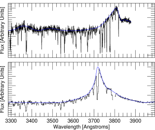
Figure 1: Spectra of 22 39 51.8 $-$29 48 37 (top, Keck+LRIS 1200/3400 grism) and 22 39 48.6 $-$29 47 49 (bottom, Keck+LRIS 400/3400 grism). Our continuum fit is indicated as a smooth blue line. The wavelength units are Å, and the flux is linear $f_{\lambda}$ from zero at the lowest major axis mark.

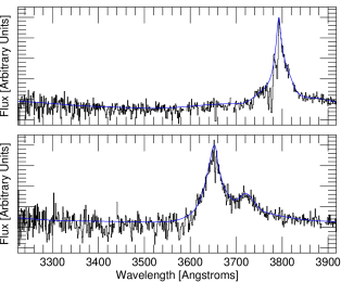
Figure 2: As Figure 1 but this time showing spectra of 14 57 56.6 +57 44 46 and 14 57 47.6 +57 44 23.5, both observed with the Lick+KAST 830/3880 grism

2.1 Systemic Redshifts

A proximity effect analysis is very sensitive to the adopted redshift for each QSO whose environment is being probed. We would like to use the systemic redshifts of the galaxies that host the QSOs, but we know that the peaks of the main UV emission lines give redshifts that are systematically smaller than these systemic redshifts by many hundreds of km s^-1, and in some cases over 1000 km s^-1, with a large QSO-to-QSO scatter (Gaskell, 1982; Tytler & Fan, 1992). A $1000$ km s^-1 redshift error corresponds to a 5 Mpc position error at $z=2$, which is large compared to the region where we expect the QSO UV radiation to be larger than the UVB, which is 3 Mpc for our median luminosity foreground QSO.

We have measured the positions of the peaks of up to three emission lines (Ly$\alpha$, CIV and MgII) for most QSOs in an attempt to get better estimates for the systemic redshifts. We measure vacuum heliocentric wavelengths, and we do not use a line when the line peak is obscured by strong absorption or the peak is not in available spectra.

The velocity shifts that we find between different emission lines are comparable but not the same as those found by others. We find that C IV gives a redshift smaller than Mg II by $753$ km s^-1, with a standard deviation (QSO to QSO $\sigma$) of $676$ km s^-1from 27 QSOs. Richards et al. (2002) finds Mg II$-$C IV $=824$ km s^-1, with $\sigma=511$ km s^-1 from a subset of 3814 SDSS QSO spectra. We find Ly$\alpha$ gives a redshift smaller by $475$ ($\sigma=455$ km s^-1) than Mg II. Guimarães et al. (2007) effectively adopt a C IV/Ly$\alpha$ offset of 750 km s^-1. Dall’Aglio et al. (2008) adopt systemic redshifts from the weak SiII+O I emission line assuming a rest wavelength of 1305.77 Å. For their eight spectra with C IV emission line coverage, this corresponds to C IV at a redshift smaller by 1190 km s^-1.

We calculate our redshifts using rest wavelengths 1215.67 Å for Ly$\alpha$, 1549.06 for C IV, and 2798.74 for Mg II. If our spectra cover Mg II, we use the redshift from that line alone (28 of our foreground QSOs). Otherwise, if our spectra cover C IV, we assign a redshift for C IV alone and then increase the redshift by 753 km s^-1(78 QSOs). Otherwise, we use the redshift from Ly$\alpha$ increased by 475 km s^-1(20 QSOs). For 4 QSOs we did not measure any of the emission lines and we list and use the redshift listed in NED. We also used this algorithm to assign redshifts to the background QSOs.

2.2 SDSS redshifts

A large number of our foreground QSOs have SDSS spectra and the SDSS project has given these QSOs redshifts derived using a template spectrum in a manner that should give the systemic redshift. For the 41 QSOs where we have both Mg II emission lines and SDSS redshifts, our redshifts are larger by 574 km s^-1 with a standard deviation of 552 km s^-1. We obtained the SDSS redshifts from the DR5 QSO catalogue (Schneider, 2007).

We only understand part of the difference in the redshifts. Our methods are considerably different. The SDSS team fit a template spectrum (Stoughton & et al., 2002) based on effective rest frame wavelengths for emission lines from Vanden Berk et al. (2001). The Vanden Berk et al. (2001) rest frame wavelengths are calculated assuming that [O III] gives the systemic redshift of the QSO. About a third of the difference is due to our differing rest frame wavelength for the Mg II emission line. We assume that Mg II is systemic, while Vanden Berk et al. (2001) assume [O III] is systemic and then find [O III]$-$Mg II$=-161$ km s^-1(Mg II gives a higher redshift than [O III]). We expect that the rest of the difference must come from the differing methods, our using line peaks vs. SDSS fitting template spectra.

We agree that [O III] should better represent the systemic redshift, but none of our QSOs have infrared spectra that can be used to measure [O III], and there is significant disagreement about the [O III] – Mg II offset. Richards et al. (2002), also using SDSS spectra, find [O III]$-$Mg II $=-97$ km s^-1, and Nestor et al. (2008) find [O III] – Mg II $=+102$ km s^-1. Unlike the SDSS spectra, which are all at low redshift so that [O III] is in the optical, the Nestor et al. (2008) were at $z\sim 2$ (like our QSOs) and have [O III] positions from NIR spectra taken by McIntosh et al. (1999) and Scott et al. (2000).

3 Method

We look for the transverse proximity effect by measuring the mean amount of absorption along the lines-of-sight to the background QSOs at redshifts near to that of the foreground QSOs. We sum the spectra of all 130 QSOs to average over the random changes in the amount of absorption in the IGM. The amount of absorption varies by factors of many over short distances, as we move in and out of absorption lines, and there are correlations that we have previously measured out to scales of 150 Mpc (Tytler et al., 2004).

We then compare the result to the expected amount of absorption for this data set. We convert the QSO magnitudes into luminosities, and we calculate the ionizing flux we expect from the foreground QSO at various distances along each background sightline. We end by examining what the foreground QSOs do to the amount of absorption in the line-of-sight to us.

Our methods differ from all early papers on the proximity effect since they counted the number of Ly$\alpha$ lines with rest frame equivalent width exceeding some minimum, and they excluded Ly$\alpha$ lines at redshifts that showed metal lines. Hence individual strong lines have a larger effect on our measurements than in the line counting method. We are also sensitive to the numerous weak lines that are below the equivalent width threshold. Such lines are easier to see where the SNR is higher, such as in the Ly$\alpha$ emission line. We will be examining the changes in the relative amount of absorption as we pass the foreground QSOs. We are then insensitive to the total amount of absorption per QSO and to global systematic errors in the continuum level.

We are sensitive to systematic errors caused by fitting the continuum differently in different parts of a spectrum. For example, the errors in our continuum may be different in and far from emission lines. This is not known to be a problem, but we can not rule out the possibility. Any systematic differences in continuum fitting over emission lines will be most noticeable in our line-of-sight proximity effect, which uses all of our data right through the Ly$\alpha$ emission line. Any errors fitting the continuum to emission lines will be less important for the transverse proximity effect. First, we restrict our analysis to wavelengths $<1200$ Å far from the peak of the Ly$\alpha$ line. In Tytler et al. (2004, Figs. 5 & 6) we showed that 1200 Å is far enough from emission line peaks to avoid unusually large continuum level errors. Second, for many of our pairs the foreground QSO redshift corresponds to a wavelength well away from any emission lines in the background QSO.

Several recent papers have detected the line-of-sight proximity effect using optical depth instead of line counting: Liske & Williger (2001), Schirber et al. (2004), Rollinde et al. (2005), Guimarães et al. (2007) and Dall’Aglio et al. (2008). Guimarães et al. (2007) and Liske & Williger (2001) used $\tau_{\rm eff}$, and their methods are similar to the methods we use here. The other papers use statistics derived from optical depth. Croft (2004) utilized the mean flux in an attempt to detect the transverse proximity effect, which is directly equivalent to our method.

We quantify the amount of absorption in our spectra with DA = $1-F/C$, where $F$ is the flux and $C$ is the continuum level. Equivalently, our DA values can be converted to effective optical depth using = ${\rm DA}=1-e^{-\tau_{\rm eff}}$, where $\tau_{\rm eff}$ is an effective optical depth. We calculate DA for each individual pixel in a spectrum, excluding of course those pixels which have been flagged for containing LLS, DLA, metal or BAL absorption. Most of the figures in this paper show DA which has been binned in some way, e.g. the DA for all the pixels in all the spectra within some redshift interval. In such cases, we find the mean DA for all the pixels in that bin from one sightline, then we average the DA values from the different sightlines.

The error we derive for a bin comes from the distribution of binned DA values, with one DA value per sightline. So when we resample, we resample the sightlines, not the individual pixels. We do the same when we estimate the error on the mean from the dispersion of the DA in individual sightlines. We do this because if we went pixel-by-pixel we would give much more weight to our higher resolution spectra. Also, taken sightline by sightline the binned DA values are statistically independent, while taken pixel-by-pixel they are not, because adjacent pixels in individual spectra are highly correlated.

DA evolves rapidly with redshift (see, for example Kirkman et al. (2007) and references therein). In Figure 3 we show the redshift evolution of DA in our data. We observe significantly different absorption at $z>2.5$ than we measured from high resolution spectra in Kirkman et al. (2007). We are not surprised by this, because line blending in the Ly$\alpha$ forest makes the continuum levels difficult to measure in low resolution spectra at higher redshift. In this case it seems that we have placed the continua too low, giving too little DA, though the sample is also getting small at high $z$ so some of the difference could be the random fluctuations in the IGM (Tytler et al., 2004).

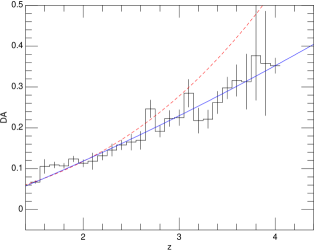
Figure 3: The DA against redshift in this data set, including both the foreground and background sightlines. The bins contain contributions from pixels between 1070 and 1170 Å in the rest frame of each QSO. The data histogram shows DA averaged over all QSOs in various redshift bins. This is intended to approximate the DA from the low density IGM. We have masked out and ignore the Ly$\alpha$ lines of LLS and DLAs and the metal absorption that we can identify. The solid blue curve shows our fit to the DA measured in this sample (Equation 1). The dashed curve shows the IGM DA measured in spectra intended for this purpose from Kirkman et al. (2007).

We fit the redshift evolution of DA in our data set with a simple power series

$${\rm DA}(z)=-0.069+0.082z+0.006z^{2}.$$ (1)

To enable us to compare data at different redshifts, the final step in our data preparation is to re-scale the DA values to those expected at $z=2$,

$${\rm DA}_{n}=(1-F/C){\rm DA}(2.0)/{\rm DA}(z),$$ (2)

where DA$(z)$ is given by Equation 1.

4 The expected line-of-sight and transverse proximity effects

We define the photoionization enhancement $\omega$ at a particular point in space due to the foreground QSO to be

$$\omega={\Gamma_{\rm QSO}\over\Gamma_{\rm UVB}}$$ (3)

where $\Gamma_{\rm QSO}$ is the photoionization rate (ionizations per H I atom per second) due to the quasar radiation, and $\Gamma_{\rm UVB}$ is the photoionization rate due to the UV background. If other factors are equal, the optical depth $\tau$ near the QSO is then given by

$$\tau={\tau_{0}\over(1+\omega)}$$ (4)

where $\tau_{0}$ is the optical depth that the IGM would have had in the absence of the foreground QSO UV flux. The linear scaling with $1+\omega$ is formally only true for the actual optical depth. The effective optical depth $\tau_{\rm eff}$ that is proportional to DA may have a slightly different scaling. For example, a high column density line on the flat part of the curve of growth will have its $\tau$ decreased when subjected to an enhanced radiation field, but its equivalent width will remain unchanged. However, we have shown in Jena et al. (2005) that at $z=2$ the effective optical depth also scales like $\tau_{\rm eff}\propto\Gamma^{-1}$, so we substitute $\tau_{\rm eff}$ for $\tau$ in Equation 4. We then calculate how the absorption changes near the QSOs using DA $=1-e^{-\tau_{\rm eff}}$.

Our assumption that $\tau_{\rm eff}=\tau_{0}(1+\omega)^{-1}$ will be valid for unsaturated lines which make much of the absorption, but we expect less sensitivity to $(1+\omega)$ for other lines. While Jena et al. (2005) found $\tau_{\rm eff}=\tau_{0}(1+\omega)^{-1}$, the spectra from their simulations with different $\Gamma$ were also consistent with a range of relationships, including the $\tau_{\rm eff}=\tau_{0}(1+\omega)^{-0.69}$ from Bolton et al. (2005). If we change the index to $-0.7$, the expected reduction in DA near the QSOs is less, by at most 0.016 which is the size of our errors on DA.

$\Gamma_{\rm QSO}$ at some distance $r=\sqrt{d^{2}+b^{2}}$ from the QSO is given by

$$\Gamma_{\rm QSO}=\int^{\infty}_{\nu_{0}}{L_{\rm QSO}(\nu)\over 4\pi r^{2}}{\sigma_{\rm HI}(\nu)\over h\nu}d\nu$$ (5)

where $L_{\rm QSO}(\nu)$ is the luminosity of the QSO as a function of frequency, $\nu_{0}$ is the Lyman limit frequency, and the H I photoinization cross section (Spitzer, 1978, Section 5.1)

$$\sigma_{\rm HI}(\nu)=6.3\times 10^{-18}\left({\nu\over\nu_{0}}\right)^{-2.75}{\rm cm}^{2}$$ (6)

Both the coefficient in front and the exponent after the $\nu/\nu_{0}$ term include the approximate effects of the Gaunt factor near 1 Ryd. Since we do not have direct observations of the Lyman limit regions for most of our QSOs, we assume that the flux distribution of each QSO is a power law $L_{\rm QSO}(\nu)=L_{\rm QSO}({\nu/\nu_{0}})^{\alpha}$, where $L_{\rm QSO}$ is the luminosity of the QSO at the Lyman limit $\nu_{0}$.

Integrating Equation 5 gives

$$\Gamma_{\rm QSO}^{12}={0.951\over 2.75-\alpha}{L_{\rm QSO}\over 4\pi r^{2}}10^{21}(10^{-12}{\rm s}^{-1}),$$ (7)

For this equation we use $\alpha=-0.5$ for the power law index to describe the continua of the QSOs.

We use $\Gamma_{\rm UVB}=1.3\times 10^{-12}$ s^-1 for all redshifts. This is the value we found in Tytler et al. (2008b) at $z=2$ by matching the observed absorption in the Ly$\alpha$ forest with the absorption seen in large hydrodynamic simulations. Bolton et al. (2005) found $\Gamma_{\rm UVB}=1.3^{+0.8}_{-0.5}\times 10^{-12}$ s^-1 at $z=2$ using a similar method. Scott et al. (2000) use the line-of-sight proximity effect to estimate $\Gamma_{\rm IGM}=1.9\pm 1\times 10^{-12}$s^-1 using all absorption and some value between 0.9 and $1.9\times 10^{-12}$s^-1 when they exclude absorption by the Ly$\alpha$ lines with associated metal lines. Haardt & Madau (2001) calculate $\Gamma_{\rm IGM}=1.33\pm 1\times 10^{-12}$s^-1 when they absorb the flux emitted by populations of QSOs and galaxies at $z=1.9$. The median redshift of our transverse proximity measurement is $z=2.2$ and the majority of our data is near that redshift. We ignore the small changes we expect in $\Gamma_{\rm IGM}$ at other redshifts.

4.1 QSO Luminosities

We compute the luminosity of each QSO at the Lyman limit (in ergs sec^-1 Hz^-1) from the observed flux density via the relation

$$L_{\rm QSO}=4\pi D_{L}^{2}(z)F_{\nu}/(1+z)$$ (8)

where $F_{\nu}$ is the observed flux density at $\lambda=(1+z)912$ Å, and $D_{L}(z)$ is the luminosity distance to redshift $z$,

$$D_{L}(z)=(1+z){c\over H_{0}}\int_{0}^{z}{dz^{\prime}\over\sqrt{\Omega_{m}(1+z^{\prime})^{3}+\Omega_{\Lambda}}}$$ (9)

We have estimated the Lyman continuum flux $F_{\nu}$ from a broadband magnitude (either $g$, $B_{J}$, or $V$) for each QSO, since in general we lack a direct measurement of $F_{\nu}$. We estimate $F_{\nu}$ by assuming each QSO has the spectrum of the HST composite QSO spectrum (Zhang et al., 1997). This is not ideal because there is significant variability in the spectral slope of individual objects, but it should be sufficient on average, which is what we need because we will always be combining many sightlines. To estimate $F_{\nu}$ for a given QSO, we compute $m$, a synthetic AB magnitude for the redshifted composite spectrum via the relation (Fukugita et al., 1996)

$$m=-2.5\log{\int d(\log\nu)AC_{\nu}(z)S_{\nu}\over\int d(\log\nu)S_{\nu}}-48.60$$ (10)

where $C_{\nu}(z)$ is the HST composite QSO spectrum at a given redshift, $S_{\nu}$ is the filter response, and $F_{\nu}=AC_{\nu}(z)$ is the observed flux. $A$ is a free parameter that is adjusted so that the synthetic magnitude is the same as the observed magnitude. $C_{\nu}(z)$ is calculated by redshifting the composite QSO spectrum, and then removing flux to simulate the mean effects of Ly$\alpha$ forest absorption, using the mean DA vs. redshift given in Kirkman et al. (2007).

Equation 10 gives AB magnitudes, which are in the same system as our $g$ band magnitudes. $B_{J}$ and $V$ magnitudes are not on the AB system, but the difference between AB and conventional magnitudes for those filters is $<0.15$ mag (Fukugita et al., 1996), and we ignore the difference in this paper and assume that all magnitudes are AB. The situation is further complicated by the fact that our QSOs with $B_{J}$ magnitudes are from the 2QZ, which has magnitudes determined from APM scans of UKST photographic plates. We do not have a response curve for that combination of filter and emulsion. Instead we have used the filter-only response for the Tyson BJ filter on the CTIO mosaic imager, which was designed to be consistent with the photographic system. For the V magnitudes we used the filter-only response for the V filter on the CTIO mosaic. For the $g$ magnitudes we used the SDSS published filter+CCD+1.2 airmass atmosphere response. The CCD and atmosphere change slowly through the filters, so their primary effect is to suppress the entire response by a nearly constant factor, and this has no net effect in Equation 10.

4.2 Distances

We compute the transverse distance $b$, the shortest distance in the plane of the sky from the background sightline to the foreground QSO, with

$$b={\phi\over(1+z)^{2}}D_{L}(z)$$ (11)

where $\phi$ is the separation between the two QSOs in radians.

To calculate the ionizing flux expected from the foreground QSO at a particular point in nearby space, we assume a Euclidean geometry and calculate the distance between the QSO and the distance $r=\sqrt{b^{2}+d^{2}}$, where $d$ is the line-of-sight distance

$$d={c\Delta z\over(1+z)H(z)},$$ (12)

where $H(z)$ is the Hubble constant at the redshift of the foreground QSO, and is given by

$$H(z)=H_{0}\sqrt{\Omega_{m}(1+z)^{3}+\Omega_{\Lambda}}.$$ (13)

or 219.73 km s^-1 at $z=2.2$.

5 Observed Absorption near the Foreground QSOs

In Figure 4 we show the average absorption (expressed as DA) near the foreground QSOs. The top panel shows the absorption observed in the line-of-sight towards the foreground QSOs, and the lower panel shows the absorption observed in the line-of-sight towards the background QSOs. In both panels, the $x$-axis is the distance in proper Mpc along a line-of-sight, with the origin at the foreground QSOs, and negative distance behind the foreground QSOs.

The top panel of Figure 4 contains contributions from pixels with rest wavelength greater than 1070 Å. The DA value for each pixel was scaled to $z=2$ using Equation 1 and then placed in the appropriate bin. The bottom panel is computed in the same way, except that only pixels with rest wavelengths between 1070 and 1200 Å in the rest frame of the background QSO were used. We use 1070 Å as the lower limit to stay well away from the O VI and Ly$\beta$ emission lines. We discuss this at length in Tytler et al. (2004). Our upper limit of 1200 Å rest is 4000 km s^-1 from the QSO, or about 20 Mpc. This is expected to be well outside the proximity region of most of our QSOs, and at this distance in no case is the UV radiation from our background QSOs expected to be more than 20% of the UV background intensity. The UV flux from our median background QSO is only about 1% of the UV background at 20 Mpc.

The curves on Figure 4 show the DA we expect to see assuming that (1) the foreground QSO radiates isotropically at the Lyman continuum, (2) the IGM density near the foreground QSO is not enhanced, and (3) the ionizing flux from the foreground QSO is either 100%, 10% or 0% of the ionizing flux inferred from the QSO magnitude. To generate the expected DA curves, we first computed the expected DA in every pixel of every sightline, and then combined the background sightlines in exactly the same way as we combined the data, preserving the $d$ values of the pixels. We add a uniform background of DA${}_{\rm metal}=0.02$ to each curve at wavelengths higher than the Ly$\alpha$ emission line. Our expected DA curves are specific to the QSO luminosities and transverse separations of the QSOs in our data set.

We see no sign of the expected proximity effect in either the line-of-sight or transverse directions. In the transverse direction we see evidence for enhanced absorption at $-6$ to $0$ Mpc. There are fewer and fewer sightlines contributing pixels at increasingly negative distances than at positive distances, so the quality of our DA measurements is significantly lower at larger negative distances in the transverse direction. In the line-of-sight direction our data is consistent with no proximity effect.

The expected transverse proximity effect would be more confined and easier to see if we had smaller redshift errors. When we calculated the expected transverse proximity effect that we show in Figure 4, we included random redshift errors with a standard deviation of 676 km s^-1. The 676 km s^-1 is the dispersion we measured in the differences between the C IV and Mg II redshifts, appropriate because we took 78 of the 130 foreground QSO redshifts from C IV. The result is that the missing absorption is spread out over many DA bins instead of being concentrated in the bins near zero. In Figure 5 we show what would be possible if we had zero error systemic redshifts for all of our foreground QSOs.

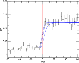
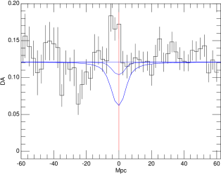
Figure 4: The proximity effect. The data histogram in the top panel shows DA averaged over all foreground QSOs as a function of distance in proper Mpc along the sightline, with the origin corresponding to the redshift of the foreground QSO. The data are in bins with width 2.5 Mpc, or 549 km s^-1 at $z=2.2$. The curves show the expected proximity effect in DA for foreground QSO UV fluxes of (top to bottom): 0, 10%, and 100% of the inferred flux at the Lyman limit. The bottom panel shows DA towards the background QSO, with the curves showing the expected transverse proximity effect. We calculate the DA we expect at various $d$ (not the 3D distance $r$) along each sightline at impact parameter $b$, using the $b$ and $d$ to calculate the QSO flux. We then sum these different expected DA curves to give the mean expected DA curves that we show, preserving distances $d$ along the line-of-sight, in the same way we sum the background QSO spectra. In calculating the expected proximity effect we have assumed that the systemic redshifts we calculate from our emission lines have random errors of $676$ km s^-1. This has the effect of smearing out the expected proximity effects – note how the zero UV flux line-of-sight proximity effect is not a step function in the presence of redshift errors.

Figure 5: The expected transverse proximity effect in the absence of $z_{\rm em}$ uncertainties. As Figure 4, but now the expected transverse proximity effect has been calculated assuming that there are no $z_{\rm em}$ errors. At $d=0$ our total data set effectively has $\omega=5.2$.

5.1 On our error estimates for the binned DA values

Each DA bin in Figure 4 contains contributions from a large number of sightlines. For the line-of-sight panel, the typical bin has contributions from about 100 QSOs. The number is not exactly 130 for each DA bin because portions of each spectra are masked to exclude DLAs, known metal absorption, and regions of bad data.

The DA bins in the transverse panel of Figure 4 typically have contributions from about 40 QSOs at negative velocities and 95 QSOs at positive velocities. The smaller number of contributions at negative distances is because our pairs were selected (for a different project) to have emission redshifts that are close to each other, so almost every sightline contributes pixels to the transverse DA at zero and positive distances, while many fewer are able to contribute pixels to the negative distance bins.

The value plotted for each distance bin is the mean of one DA value from each of the sightlines with data at the appropriate distance. The sightlines are given equal weight. For each bin, we take the error bar to be the standard error on the mean: the standard deviation of the contributing sightlines divided by the square root of the number of contributing sightlines. We have also estimated the error for each bin via bootstrap resampling, and the two methods are consistent with each other for all bins to better than 10%.

In Figure 6 we show the distribution of DA values measured over 2.5 Mpc for all of the points that went into the transverse panel of Figure 4. In Figure 7 we show the distribution of sightline DA values for three of the individual distance bins. The distributions do not look like a normal distribution because the flux probability distribution function (FPDF) is highly non-normal (Kim et al., 2007; Tytler et al., 2008b). We work with the distribution of the mean fluxes in the 2.5 Mpc bins, so our distributions are much closer to a normal distribution than they are to the underlying full-resolution FPDF, as shown for simulated spectra by Tytler et al. (2008b, Figs. 10 & 19) and as expected by the central limit theorem.

The central limit theorem also guarantees that if we take a large number of samples from the distribution shown in Figure 6, that the mean value with be normally distributed with a standard deviation given by the standard error on the mean (e.g. our error bars). The distributions we observe for individual bins in Figure 7, as well as the fact that the distribution observed in Figure 6 is not wildly different from a normal distribution, give us confidence that the errors we have presented in Figure 4 are reasonable.

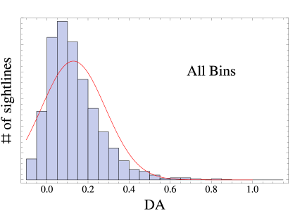
Figure 6: The distribution of DA values, each given by the mean DA measured over 2.5 Mpc in one sightline, for all of the values that are contained in the transverse panel of Figure 4. The red curve curve shows a normal distribution centred on the mean of these values with the standard deviation given by these values.

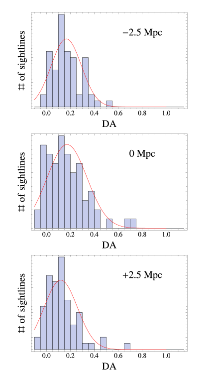
Figure 7: As Figure 6, but showing only the values contributing to the transverse bins centred at -2.5, 0, and 2.5 Mpc.

We measure the covariance for adjacent 2.5 Mpc bins in our transverse DA data to be 20% of the variance in each bin. The covariance drops to 5% two bins out. This is a bit higher than expected purely from the large scale structure of the Ly$\alpha$ forest (Kirkman et al., 2007), where we found that the covariance at 550 km s^-1 (about 2.5 Mpc) was 6% of the value at 50 km s^-1 at $1.0<z<1.5$. The excess covariance in our sample may be due in part to its higher redshift, but it probably also reflects errors in our data handling, including continuum fitting errors and residuals from unmasked LLS and metal line absorption. The bin-to-bin covariance is large enough that is should be taken into account when attempting to determine the significance of any feature in our DA data.

6 Line-of-sight Proximity Effect Discussion

We see in Figure 4 that we expect a relatively small line-of-sight proximity effect, because our QSOs are fainter by a factor of few than those in past work. Our QSOs have a median Lyman Limit luminosity of 3.3$\times 10^{30}$ ergs s^-1 Hz^-1, which is fainter by a factor of six compared to the Guimarães et al. (2007) sample. Four of the 10 Liske & Williger (2001) QSOs are more luminous than ours by a factor $>6.7$, and the others are more luminous by a factor of $\sim 2$.

We still expect to readily detect the proximity effect but we see no change in the amount of H I absorption as we approach the foreground QSOs. This absence of the line-of-sight proximity effect is unexpected, but not completely surprising because others have recently reported reduced effects, and we have a ready qualitative explanation if the gas density near to the QSOs is enhanced by a factor of a few.

QSOs are expected to form in dense environments. Serber et al. (2006) find that the galaxy density within 100 kpc of $z<0.4$ QSOs is between 1.4 and 3 times the galaxy density around L^∗ galaxies, and that the overdensity persists at some level out to 1 Mpc. The environments around QSOs at $z=2.2$ may be significantly different, as clustering will be less developed, and different types of galaxy may show QSO activity. IGM calculations indicate the mean gas density may be enhanced by a factor of a few within about 3 Mpc of a QSO (Loeb & Eisenstein, 1995; Faucher-Giguère et al., 2008) – this is approximately the factor we need to explain our non-detection of the line-of-sight effect. The IGM Ly$\alpha$ opacity will vary approximately as the square of the gas density – one factor for the increased density, and another for the increased neutral fraction. Hence a factor of 3 increase in density will give about a factor of 9 more H I absorption, which will change the expected proximity effect to approximately that for QSOs with 10% of their observed UV luminosities. The curve in Figure 4 for this reduced luminosity is consistent with the data, given the uncertainties over the redshifts.

Rollinde et al. (2005) also saw less proximity effect than expected and they deduced that the gas density might be enhanced by “a factor of a few” near to their QSOs. Guimarães et al. (2007) saw a reduced proximity effect towards more luminous QSOs at higher redshifts and they claim that they need a significant density enhancement over a much larger region of $\sim 21$ Mpc, more than expected from simulations.

If the gas density is a factor of a few higher around QSOs and does not depend on QSO luminosity at a given redshift, then the density enhancement will have a larger impact on less luminous QSOs because the distance to which the QSO flux dominates the UVB flux is then smaller than for more luminous QSOs. This might explain why earlier papers (Carswell et al., 1982; Bajtlik et al., 1988; Scott et al., 2000) readily saw the line-of-sight proximity effect around QSOs that were more luminous than ours. However, the different results might instead come from the different methods. Our methods and those of Rollinde et al. (2005) and Guimarães et al. (2007), who also claimed enhanced density near to QSOs, are based on flux, while the early papers that saw the expected line-of-sight proximity effect used line counting. To our knowledge, no one has attempted a proximity effect analysis on the same data set using both line counting and continuous optical depth methods, so it is possible that the two methods give systematically different results.

6.1 Other possible explanations for why we do not see a line-of-sight proximity effect

While we are happy to entertain the idea that enhanced density explains why we do not see the line-of-sight proximity effect that we expect, we have not directly shown that this is the case. It remains surprising that the enhanced ionization – density cancellation is perfect within our measurement errors. Here we explore other possible explanations for what we see.

In addition to enhanced density near our foreground QSOs, it may be possible to explain our lack of an observed proximity effect in other ways. In particular, Figure 4 shows that the line-of-sight data is roughly compatible with $\omega$ values 10 times smaller than we expect. This could be achieved, for example, if the UV background is a factor of 10 higher than we expect. However, our work on the UVB from Ly$\alpha$ forest absorption Tytler et al. (2004); Jena et al. (2005); Tytler et al. (2008b), the Bolton et al. (2005) results using similar methods, and the Haardt & Madau (2001) result derived by counting UV sources all suggest that $\Gamma_{\rm UVB}$ is less than a factor of two higher than the value of $\Gamma_{\rm UVB}=1.3\times 10^{-12}$ s^-1 that we have adopted. We believe that the 50% error claimed by Bolton is more reasonable than a factor of two, and hence we think that it is unlikely that our result will be explained by a higher than expected UVB.

The flux enhancement near the foreground QSOs, $\omega$, could be lower than we expect if these QSOs were less luminous in the recent past than they are today. At a distance from a QSO where the QSO UV radiation is twice that of the UVB, we expect it to take 10 kyr ($(2\Gamma_{\rm UVB})^{-1}$) for the ionization of the gas to respond to increased UV flux from the QSO, so $\omega$ can be different than we expect if QSOs are highly variable on timescales short compared to 10 kyr. We are presumably more likely to discover and observe bright QSOs, so if QSOs are varying on short timescales the sense of this effect may on average lower $\omega$.

On time-scales of days to years, QSOs are more variable at smaller UV wavelengths and at lower luminosities (Vanden Berk et al., 2004). Over tens of years in the rest frame, the rest frame UV flux varies by $>1.5$ magnitudes for 50% of QSOs and by $>3$ mag for 9% of QSOs (Heckman, 1976). de Vries et al. (2003); de Vries et al. (2005) find that QSOs undergo bursts of 2-magnitudes on periods of years, with larger variations on longer time scales and for less luminous QSOs, all roughly consistent with accretion disk instabilities. The structure function describing the variability of all QSOs rises monotonically at a constant rate out to 40 years in the QSO rest frame with no turnover (de Vries et al., 2005; de Vries et al., 2006) – the preferred time scale for QSO variation is at least this long. If the same random walk has continued, then many QSOs could be factors of ten times less luminous 10 kyr ago. But Martini & Schneider (2003) estimate that QSO UV luminous episodes typically last $>20,000$ years, on the assumption that a given QSO seen on the POSS-I plates was either on or off (absolute magnitude fainter than -23) at the epoch of the SDSS observation.

Our adopted redshifts may differ systematically from the QSO systemic redshifts. To give the full expected proximity effect we would need to increase the QSO redshifts by 800 km s^-1, moving the origin on the figures to the left by 1.5 data bins or 3.5 Mpc. Given that our redshifts come either directly, or indirectly from Mg II, this seems an incredibly large error, which would imply that the C IV lines in our QSOs have typical blueshifts of 1550 km s^-1 and not the 753 km s^-1 that we assume.

Another alternative explanation is that part of the line-of-sight proximity effect is masked by extra H I absorption that is not from the IGM. It is well known that there is an excess of absorption systems that show C IV lines with redshifts similar to QSO emission redshifts. Tytler et al. (2008a, Fig. 7a) showed these excess systems for a super-set of the QSOs that we use here. Hennawi et al. (2006) show there is also a strong excess of LLS and DLAs with redshifts similar to the QSOs. In addition Wild et al. (2008) find that $>$ 40% of C IV absorbers within 3000 km s^-1 of a QSO are directly associated with the QSO itself and do not arise in the IGM. These systems will nearly all have strong Ly$\alpha$ absorption lines that will tend to hide the line-of-sight proximity effect.

In general, the extra absorption near the QSO redshift is a specific example of the idea that the gas density is higher near to the QSOs. In early work on the proximity effect (Carswell et al., 1982; Tytler, 1987; Bajtlik et al., 1988), all Ly$\alpha$ lines that had associated metal lines were excluded, hence removing this non-IGM “contamination” at all redshifts. This was not done in later work (Scott et al., 2000, 2002; Dall’Aglio et al., 2008). Scott et al. (2002, § 6) found that removing “associated absorbers, damped Ly$\alpha$ absorbers, and blazars” from their low redshift proximity effect analysis decreased the UVB needed to explain the proximity effect by a factor of two. This factor of two reduction seems desirable (Faucher-Giguère et al., 2008, Fig. 1), because the UVB from the proximity effect then matches that inferred by matching the observed DA to large hydrodynamic simulations (Bolton et al., 2005; Tytler et al., 2008b).

For this paper we have attempted to remove only part of the Ly$\alpha$ absorption associated with metal systems, that where the Ly$\alpha$ lines are DLAs or other prominent Ly$\alpha$ lines. We have not removed the Ly$\alpha$ lines of other metal systems, and we do not know whether these could significantly or totally cancel out the line-of-sight proximity effect.

We could also speculate that our QSOs might show more than the typical amount of extra metal systems with redshifts similar to the QSO redshifts, perhaps because they are lower luminosity QSOs. This is hinted because X-ray absorption is more common in lower luminosity AGN.

7 Transverse Proximity Effect Discussion

We now describe the transverse proximity data in Figure 4, and we discuss the issues that carry across from our interpretation of the line-of-sight proximity effect. We end with new factors that are specific to the transverse proximity effect.

The first point to make is that the spectra that we sum for the transverse plot are the different than the ones we use for the line-of-sight. In the transverse direction we use the spectrum of the background QSO, while for the line-of-sight we use the spectrum of the foreground QSO. Hence the noise characteristics are similar, but not identical. As we previously explained, we lose spectra as we move farther behind the foreground QSOs on the transverse plot, which explains why the errors are nearly constant to the right but increase going to the left of zero.

The second point is that we see no change in the amount of absorption as we approach the QSOs from the Earth side, from the right. This seems reasonable because we also did not see any change in the absorption in the line-of-sight to these same QSOs. The same explanation that we gave for the lack of the line-of-sight proximity effect may apply to the lack of change in the transverse absorption, because we are probing similar distances with both the foreground and the background QSO light. Hence we propose that we do not see either the line-of-sight proximity, or the transverse proximity on the near side of the foreground QSO, because the enhanced from ionization the UV flux from the foreground QSO is cancelled by higher gas density near to those QSOs.

We discussed other possible explanations for the lack of the line-of-sight proximity effect. While arbitrarily large systematic errors in the redshifts of the foreground QSOs might enhance, diminish or remove the line-of-sight proximity effect, redshift errors have much less effect on the transverse effect, because we can now also see absorption from behind the foreground QSO. Systematic errors in the foreground QSO emission redshifts will again move the zero point to the left or right on the plot, but this has little effect because the absorption we observe and expect does not change significantly when we apply realistic shifts in the zero point.

Random redshift errors do not change the total amount of absorption, but they do re-distribute that absorption into more pixels. In Figure 5 we re-calculate the expected transverse proximity effect assuming that we have no errors in the QSO redshifts. We see a deeper and narrower expected drop in H I absorption.

Extra Ly$\alpha$ absorption for the excess of metal line systems with redshifts close to the redshift of the background QSO will have little impact on the transverse proximity effect, except when the two QSOs have similar redshifts. The extra absorption near to the foreground QSO is one manifestation of the enhanced density that we believe is important. Associated absorbers ejected by the foreground QSOs are not expected to reach the sightline to the background QSO.

The third point about the transverse plot is that we see extra absorption starting at the foreground QSO position and extending about 6 Mpc behind the foreground QSO. We regard this as significant for two reasons. First, we see a 2 – 3 $\sigma$ excess over 3 pixels, extending from $-6.25$ to $+1.25$ Mpc. Second, we had earlier decided that the lack of the expected line-of-sight proximity effect was significant, and that the lack of the expected transverse proximity effect on the front side of the foreground QSOs was also significant. These two lacks involve approximately the same deviations from the data as does the excess absorption behind the QSOs. Hence we should also regard the excess absorption as significant. This argument relates to the Bayesian preference that we not change our prior evaluation, of what would constitute a significant result, after we see the data. Rather we should hold a consistent set of beliefs about probabilities before and after we obtain the data, striving for diachronic probabilistic coherence. While we have a significant detection of excess absorption, we are less sure of the precise location of the excess because random and especially systematic redshift errors can move the apparent location of the absorption. At least some of the excess is behind the foreground QSOs.

The asymmetry between the amount of absorption in front of and behind the foreground QSOs could only be seen in the transverse analysis, because the line-of-sight analysis is only sensitive to absorption in front. We also require a large sample of close pairs of QSOs to see this effect, with emission redshifts at least as good as we have. It is clear from Figure 4 that it would be hard to see this asymmetry in a much smaller sample.

8 Implications of anisotropic absorption

The transverse sightlines in Figure 4 suggest that there is more absorption behind the foreground QSOs than there is in front. If this result is correct it may have significant implications, some of which we now discuss.

The amount of excess absorption behind the QSOs is numerically similar in size to the lack of absorption that we had expected. This immediately suggests that the excess absorption is coming from an enhancement of the gas density that is the same size as the enhancement that we already invoked on the near side of the QSO. We expect the density distribution to be isotropic about the QSOs, when we average over many QSOs. We can then explain the enhanced absorption using the same density enhancement, but with no UV radiation from the foreground QSO reaching the gas behind the foreground QSOs before the absorption occurred. We can not say precisely how much the flux behind the foreground QSOs needs to be suppressed, but we can see from Figure 4 that if $\omega$ is down by about a factor of 10 behind the QSO, and we have a symmetric density enhancement centred on the QSOs, then we would expect to see something similar to our observed data.

There are two commonly discussed ways of limiting the amount of UV flux seen by the gas behind the foreground QSOs. First, the QSO emission might be anisotropic. Second, the QSO may have a short episodic lifetime. We will discuss both possibilities.

8.1 Anisotropic UV emission?

Common AGN unification models frequently contain an obscuring torus surrounding a central continuum source and broad emission-line gas (e.g. (Barthel, 1989; Antonucci, 1993)). In this scenario, QSO UV emission is expected to be highly anisotropic, with the UV emission strongest along the poles of the system when the obscuring torus defines the equator. But while an obscuring torus could explain a general lack of ionizing photons in the transverse direction, it does not explain why there may be fewer ionizing photons behind the QSO than in front, because the UV radiation should escape equally from both sides of the torus.

We can break the axial symmetry in the UV emission if the obscuration around the QSOs covers most sight lines, leaving only a few holes unobscured, including the hole sending UV in our direction, a modification of the cloudy torus model of Nenkova et al. (2008). A single hole of diameter of order 60 – 120 degrees seen from the QSO might explain our data. Here 60 degrees is the minimum to illuminate enough of the volume in front of the QSO, while larger than 120 degrees leads to too much flux behind the QSOs since the line-of-sight to us is often far from the centre of the hole. This model is effectively similar to a hypothetical accretion disk that emits UV from one side but not the other. Models with several smaller unobscured holes are not favored because they do not give much less flux behind the QSOs.

We might explain the excess absorption behind the QSOs if the UV flux behind the average QSO is of order 10% or less of the flux we see. A single unobscured hole of diameter 60 – 120 degrees covers a fraction of 0.25 – 0.43 of the sky seen from a QSO. We expect this fraction is related to the fraction of all QSOs that are type 1 rather than type 2. For Seyfert galaxies, Schmitt et al. (2001) estimate 0.3 while Hao & et al. (2005) find 0.5. This fraction rises with luminosity reaching of order 0.8 for QSOs (Maiolino et al., 2007; Barger et al., 2005). We might reconcile this high fraction of unobscured QSOs with our need for more obscuration because we need block only the Lyman continuum flux, and not the entire UV and optical. The obscuration we need does not necessarily lead to high mid-infrared to optical flux ratios used to calculate the fraction of 0.8.

8.2 Short episodic lifetimes?

A second option is that the QSOs have not been emitting for long enough to have illuminated the volume probed behind. In this case the asymmetry is caused by the extra time for the UV radiation from the foreground QSO to reach the gas behind, and to do this before the light from the background QSO passes through that gas.

We can account for the excess absorption behind the foreground QSOs if they have had their current UV luminosities for approximately 1 Myr, and prior to then, for $>40$ Myr, they were a factor of $\sim 10$ less luminous. We work in the QSO frame, so that “today” refers to the time in the QSO frame when the light that we see left the QSO; hence we ignore the time for light to travel from the QSO to us, and we can ignore the $(1+z)$ time dilation would apply if we were to shift to our frame. Our closest sightlines are separated by $\sim 0.1$ Mpc, corresponding to a light propagation time of $\sim 0.32$ Myr, while our median sightline is separated by 1.25 Mpc or 4.1 Myr. The typical foreground QSO must have emitted the flux that we deduce for at least 4.1 Myr if that flux is to reach the closest approach of the line-of-sight from the background QSO. Longer is needed to illuminate the parts of the background QSO line-of-sight that are behind (at higher redshift than) the foreground QSO. The surface that is illuminated by radiation that left the foreground QSO $t$ Myr ago is a paraboloid with the QSO at the focus and the vertex $t/2$ million light-years behind the QSO, as shown in Adelberger (2004, Fig. 3), Visbal & Croft (2008, Fig. 1), and Tytler et al. (2008a, Fig. 24)). We demonstrate this in Figure 8.

We can obtain approximate limits on the QSO episodic lifetime from the distribution of absorption around the foreground QSOs. If the QSOs had at least their current luminosity for more than 10 Myr, then regions that are approximately 1.2 Mpc behind the foreground QSO (and at the median sky separation) would have experienced the QSO flux, and we might expect that we would not see excess absorption in the bin centred on zero. Hence we can deduce, because of the excess absorption in the zero bin, that the typical QSO episodic lifetime is $<10$ Myr.

On the other extreme, we note that the bins in front of the QSO do not show enhanced absorption. If we assume that the IGM density enhancement is symmetric in front of and behind the foreground QSOs, the lack of extra absorption in the bins in front of the foreground QSO can be taken as evidence that they have been illuminated by the QSO. For our median separation, it will take $\sim 0.3$ Myr for the QSO to illuminate the bin sampling 1.25 – 3.75 Mpc in front of the QSO. Hence we can deduce that the typical QSO episodic lifetime is $>0.3$ Myr.

Taken together, the transverse absorption in front of and behind the foreground QSOs suggest a QSO episodic lifetime $0.3<t_{e}<10$ Myr, or $t_{e}\sim 1$ Myr. Again, a given QSO might have several or many epochs with high UV luminosity. Hence the 1 Myr episodic lifetime refers to the time since the start of the latest QSO outburst and not to the total QSO lifetime.

This model also gives the approximate minimum time the QSOs should have been in their low UV luminosity “off states” prior to the current UV bright episode. To avoid illuminating the bin furthest behind the QSOs with excess absorption at $d=-6.25$ to $-3.75$ Mpc at the typical $b=1.25$ Mpc, we need the QSOs in the off state for $>40$ Myr. If we knew the distribution of density near the QSOs, and we had more accurate redshifts, we could make a more accurate estimate of how long the QSOs have had their current UV luminosities, and the minimum length of the off state.

Our conclusion that we are seeing evidence for $\sim 1$ Myr QSO episodic lifetimes hinges on our observation of increased absorption behind the QSO but not in front of it. In an earlier analysis of the transverse proximity effect, Croft (2004) found enhanced absorption on both sides of the QSO. He had few close sightlines and convolved his observed absorption with a 7 Mpc Gaussian filter, but it is clear that the excess absorption is centred near to the redshift of the foreground QSO. We can not explain the discrepancy between our results and the Croft (2004) results, but the differences between our assumed systemic redshifts and the systemic redshifts used by SDSS may be part of the difference.

We note that if we were to increase our foreground redshift by 550 km s^-1 to centre the excess absorption at 0 Mpc, we would observe a significant line-of-sight proximity effect. But we would then have the problem that on average, our C IV emission lines would be at the systemic redshift of the QSO, and we discussed in §2.1 this is inconsistent with multiple observations. We also think this unlikely because Tytler et al. (2008b) see excess C IV absorbers at velocities $\sim 300\pm 150$ km s^-1 in front of a superset of the QSOs we study here. If we move all the QSOs back 550 km s^-1 these excess C IV absorbers would be at $\sim 850$ km s^-1 in front of the QSOs, which would be hard to explain. Rather, the C IV absorption suggest that we might move the QSO redshifts in the other direction, decreasing them by $\sim 300$ km s^-1 to approximately centre the C IV on the QSOs. This would move the origin in Figure 4 one half bin to the right, putting the extra H I absorption entirely behind the QSOs.

8.3 Are short episodic lifetimes plausible?

It has long been speculated that QSOs may exhibit highly intermittent activity. Shields & Wheeler (1978) showed that the storage and release of gas in an accretion disk would produce just such activity. Disk instabilities are likely to produce variation on many time scales, from $10^{1}$ – $10^{6}$ yrs (Wallinder et al., 1992). But it is also the case that the characteristic e-folding time for a black hole to increase its mass by accretion is 45 Myr when its luminosity is the Eddington value and the radiative efficiency is 0.1 (see review by Martini (2004)). If such accretion is the dominant mode of black hole growth, then we expect a given high mass black hole to be UV luminous for of order $10^{8}$ yr in total, but we do not know whether this manifests as one long episode or many shorter bursts.

Goodman (2003) finds that there are no obvious ways to have accretion disks around giant black holes that are stable against fragmentation at large radii. Consequently, he suggests that disks do not exist much beyond 0.01 pc or 1000 Schwartzschild radii. Such small disks would be depleted onto the black hole in $<1$ Myr, implying the typical UV luminosities 1 Myr ago could have been at least an order of magnitude less, as we require to explain the excess Ly$\alpha$ absorption behind the QSOs.

The excess absorption seen behind the QSOs might be a detection of instabilities in accretion disks on Myr time-scales (Czerny, 2006). Janiuk et al. (2004) discuss how the thermal-viscous instability in standard $\alpha-$accretion disks can lead to outbursts of $10^{4}$ yr duration for a $10^{8}$ $M_{\odot}~{}$ black hole. McHardy et al. (2006) support the old idea (Shakura & Sunyaev, 1976) that AGN are scaled up Galactic stellar mass black hole systems because they can predict the time scale of the break in the power spectrum density of the X-ray fluxes from the black hole mass and luminosity or accretion rate (see also Fender et al. (2007)). Done & Gierliński (2005) discuss how the transitions between the different states of accretion luminosity seen in Galactic stellar mass black holes may manifest in $10^{9}$ $M_{\odot}~{}$ QSOs as transition into low luminosity states on time-scales of 0.3 Myr.

If we combine these arguments with the large amplitudes of the observed short-term variability, the lack of a turn-over in the structure function out to tens of years, the increase in variability as smaller UV wavelengths (all discussed in §6.1), we find it reasonable to postulate that our sample of QSOs have episodic life-times $\sim 1$ Myr in the QSO rest frame. Prior to the current episode, for perhaps tens of Myrs, their Lyman continuum luminosity was at least a factor of ten less than today.

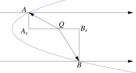
Figure 8: The regions of space around a QSO that will show enhanced ionization in the spectra of background objects, if the QSO has some fixed episodic lifetime, and the medium is at all times highly ionized. Absorbers to the right of the blue parabola will have seen enhanced ionization from the QSO before the light from the background object arrives. Light from the background objects (horizontal lines) will arrive at absorbers to the left of the parabola before the UV flux from the QSO arrives. In the frame of the QSO, light from a background object will arrive at point $A$ a time in the past equal to the light travel time from $A_{s}$ to $Q$, which we denote as $t(A_{s}Q)$. We take the light travel time as positive. So point $A$, on the boundary of the illuminated volume, can be found by requiring that $t(AQ)+t(A_{s}Q)=T$, where $T$ is the episodic lifetime of the QSO. The same argument applies for $B$, but because light from a background object arrives at point $B$ at a time in the future with respect to the QSO frame, we have $t(BQ)-t(QB_{S})=T$. Taking the set of points similar to $A$ and $B$ at all impact parameters gives the blue parabola. Light emitted from the foreground QSO $T$ years ago, arrives on the parabola at the same time as the light from the background QSO that we see.

Acknowledgments

We thank the anonymous referee for many very helpful suggestions and criticisms. We thank Arlin Crotts for providing us with some of the spectra used in this paper, which he obtained from NOAO facilities, operated by AURA for the NSF. Former UCSD students John O’Meara and Nao Suzuki helped to obtain some of the spectra used in this paper. We thank Mike Fall, Jeremy Goodman, Matt Malkan, Jason Prochaska, Don Schneider, Greg Shields, Chuck Steidel and Gordon Richards for important discussions. The bulk of the data were obtained using the Kast spectrograph on the Lick Observatory 3m-Shane telescope, the LRIS spectrograph on the Keck-I telescope, and the SDSS archive. The W.M. Keck Observatory is operated as a scientific partnership among the California Institute of Technology, the University of California and the National Aeronautics and Space Administration and was made possible by the generous financial support of the W.M. Keck Foundation. We are exceedingly grateful for the help we receive from the staff at both observatories. We recognise and acknowledge the very significant cultural role and reverence that the summit of Mauna Kea has always had within the indigenous Hawaiian community. We are extremely grateful to have the opportunity to conduct observations from this mountain. This research has made use of the NASA/IPAC Extragalactic Database (NED) which is operated by the Jet Propulsion Laboratory, California Institute of Technology, under contract with the National Aeronautics and Space Administration. Funding for the creation and distribution of the SDSS Archive has been provided by the Alfred P. Sloan Foundation, the Participating Institutions, the National Aeronautics and Space Administration, the National Science Foundation, the U.S. Department of Energy, the Japanese Monbukagakusho, and the Max Planck Society. The SDSS Web site is http://www.sdss.org/. This work was funded in part by NSF grants AST-0098731, 0507717 and 0808168 and by NASA grant NAG5-13113.

References

- Adelberger (2004) Adelberger K. L., 2004, ApJ, 612, 706
- Antonucci (1993) Antonucci R., 1993, ARAA, 31, 473
- Bajtlik et al. (1988) Bajtlik S., Duncan R. C., Ostriker J. P., 1988, ApJ, 327, 570
- Barger et al. (2005) Barger A. J., Cowie L. L., Mushotzky R. F., Yang Y., Wang W.-H., Steffen A. T., Capak P., 2005, AJ, 129, 578
- Barthel (1989) Barthel P. D., 1989, ApJ, 336, 606
- Bolton et al. (2005) Bolton J. S., Haehnelt M. G., Viel M., Springel V., 2005, MNRAS, 357, 1178
- Bowen et al. (2006) Bowen D. V., Hennawi J. F., Ménard B., Chelouche D., Inada N., Oguri M., Richards G. T., Strauss M. A., Vanden Berk D. E., York D. G., 2006, ApJ, 645, L105
- Carswell et al. (1987) Carswell R. F., Webb J. K., Baldwin J. A., Atwood B., 1987, ApJ, 319, 709
- Carswell et al. (1982) Carswell R. F., Whelan J. A. J., Smith M. G., Boksenberg A., Tytler D., 1982, MNRAS, 198, 91
- Coil et al. (2007) Coil A. L., Hennawi J. F., Newman J. A., Cooper M. C., Davis M., 2007, ApJ, 654, 115
- Croft (2004) Croft R. A. C., 2004, ApJ, 610, 642
- Croom et al. (2005) Croom S. M., Boyle B. J., Shanks T., Smith R. J., Miller L., Outram P. J., Loaring N. S., Hoyle F., da Ângela J., 2005, MNRAS, 356, 415
- Czerny (2006) Czerny B., 2006, in Gaskell C. M., McHardy I. M., Peterson B. M., Sergeev S. G., eds, Astronomical Society of the Pacific Conference Series Vol. 360 of Astronomical Society of the Pacific Conference Series, The Role of the Accretion Disk in AGN Variability. pp 265–+
- Dall’Aglio et al. (2008) Dall’Aglio A., Wisotzki L., Worseck G., 2008, A&A, 480, 359
- de Vries et al. (2003) de Vries W. H., Becker R. H., White R. L., 2003, AJ, 126, 1217
- de Vries et al. (2006) de Vries W. H., Becker R. H., White R. L., 2006, in Gaskell C. M., McHardy I. M., Peterson B. M., Sergeev S. G., eds, Astronomical Society of the Pacific Conference Series Vol. 360 of Astronomical Society of the Pacific Conference Series, Long-Term Optical Quasar Variability. pp 29–+
- de Vries et al. (2005) de Vries W. H., Becker R. H., White R. L., Loomis C., 2005, AJ, 129, 615
- Done & Gierliński (2005) Done C., Gierliński M., 2005, MNRAS, 364, 208
- Faucher-Giguère et al. (2008) Faucher-Giguère C.-A., Lidz A., Zaldarriaga M., Hernquist L., 2008, ApJ, 673, 39
- Fender et al. (2007) Fender R., Koerding E., Belloni T., Uttley P., McHardy I., Tzioumis T., 2007, ArXiv e-prints, 706
- Fukugita et al. (1996) Fukugita M., Ichikawa T., Gunn J. E., Doi M., Shimasaku K., Schneider D. P., 1996, AJ, 111, 1748
- Gallerani et al. (2008) Gallerani S., Ferrara A., Fan X., Choudhury T. R., 2008, MNRAS, 386, 359
- Gaskell (1982) Gaskell C. M., 1982, ApJ, 263, 79
- Giallongo et al. (1996) Giallongo E., Cristiani S., D’Odorico S., Fontana A., Savaglio S., 1996, ApJ, 466, 46
- Gonçalves et al. (2008) Gonçalves T. S., Steidel C. C., Pettini M., 2008, ApJ, 676, 816
- Goodman (2003) Goodman J., 2003, MNRAS, 339, 937
- Guimarães et al. (2007) Guimarães R., Petitjean P., Rollinde E., de Carvalho R. R., Djorgovski S. G., Srianand R., Aghaee A., Castro S., 2007, MNRAS, 377, 657
- Haardt & Madau (2001) Haardt F., Madau P., 2001, in Clusters of galaxies and the high redshift universe observed in X-rays, Recent results of XMM-Newton and Chandra, XXXVIth Rencontres de Moriond, XXIst Moriond Astrophysics Meeting, March 10-17, 2001, Savoie France. Edited by D.M. Neumann & J.T.T. Van Modelling the UV/X-ray cosmic background with CUBA
- Hao & et al. (2005) Hao L., et al. 2005, AJ, 129, 1795
- Heckman (1976) Heckman T. M., 1976, PASP, 88, 844
- Hennawi & Prochaska (2007) Hennawi J. F., Prochaska J. X., 2007, ApJ, 655, 735
- Hennawi et al. (2006) Hennawi J. F., Prochaska J. X., Burles S., Strauss M. A., Richards G. T., Schlegel D. J., Fan X., Schneider D. P., Zakamska N. L., Oguri M., Gunn J. E., Lupton R. H., Brinkmann J., 2006, ApJ, 651, 61
- Jakobsen et al. (2003) Jakobsen P., Jansen R. A., Wagner S., Reimers D., 2003, A&A, 397, 891
- Janiuk et al. (2004) Janiuk A., Czerny B., Siemiginowska A., Szczerba R., 2004, ApJ, 602, 595
- Jena et al. (2005) Jena T., Norman M. L., Tytler D., Kirkman D., Suzuki N., Chapman A., Melis C., Paschos P., O’Shea B., So G., Lubin D., Lin W., Reimers D., Janknecht E., Fechner C., 2005, MNRAS, 361, 70
- Kim et al. (2007) Kim T.-S., Bolton J. S., Viel M., Haehnelt M. G., Carswell R. F., 2007, MNRAS, 382, 1657
- Kim & Croft (2008) Kim Y.-R., Croft R. A. C., 2008, MNRAS, 387, 377
- Kirkman et al. (2007) Kirkman D., Tytler D., Lubin D., Charlton J., 2007, MNRAS, 376, 1227
- Kirkman et al. (2007) Kirkman D., Tytler D., Lubin D., Charlton J., 2007, MNRAS, 376, 1227
- Kirkman et al. (2005) Kirkman D., Tytler D., Suzuki N., Melis C., Hollywood S., James K., So G., Lubin D., Jena T., Norman M. L., Paschos P., 2005, MNRAS, 360, 1373
- Liske & Williger (2001) Liske J., Williger G. M., 2001, MNRAS, 328, 653
- Loeb & Eisenstein (1995) Loeb A., Eisenstein D. J., 1995, ApJ, 448, 17
- Maiolino et al. (2007) Maiolino R., Shemmer O., Imanishi M., Netzer H., Oliva E., Lutz D., Sturm E., 2007, A&A, 468, 979
- Martini (2004) Martini P., 2004, in Ho L. C., ed., Coevolution of Black Holes and Galaxies QSO Lifetimes. pp 169–+
- Martini & Schneider (2003) Martini P., Schneider D. P., 2003, ApJL, 597, L109
- McHardy et al. (2006) McHardy I. M., Koerding E., Knigge C., Uttley P., Fender R. P., 2006, Nature, 444, 730
- McIntosh et al. (1999) McIntosh D. H., Rix H.-W., Rieke M. J., Foltz C. B., 1999, ApJL, 517, L73
- Nenkova et al. (2008) Nenkova M., Sirocky M. M., Nikutta R., Ivezic Z., Elitzur M., 2008, arXiv:0806.0512
- Nestor et al. (2008) Nestor D., Hamann F., Hidalgo P. R., 2008, MNRAS, 386, 2055
- Richards et al. (2002) Richards G. T., VandenBerk D. E., Reichard T. A., Hall P. B., Schneider D. P., SubbaRao M., Thakar A. R., York D. G., 2002, AJ, 124, 1
- Rollinde et al. (2005) Rollinde E., Srianand R., Theuns T., Petitjean P., Chand H., 2005, MNRAS, 361, 1015
- Schirber et al. (2004) Schirber M., Miralda-Escudé J., McDonald P., 2004, ApJ, 610, 105
- Schmitt et al. (2001) Schmitt H. R., Antonucci R. R. J., Ulvestad J. S., Kinney A. L., Clarke C. J., Pringle J. E., 2001, ApJ, 555, 663
- Schneider (2007) Schneider D. P. et al., 2007, AJ, 134, 102
- Scott et al. (2000) Scott J., Bechtold J., Dobrzycki A., Kulkarni V. P., 2000, ApJS, 130, 67
- Scott et al. (2002) Scott J., Bechtold J., Morita M., Dobrzycki A., Kulkarni V. P., 2002, ApJ, 571, 665
- Serber et al. (2006) Serber W., Bahcall N., Ménard B., Richards G., 2006, ApJ, 643, 68
- Shakura & Sunyaev (1976) Shakura N. I., Sunyaev R. A., 1976, MNRAS, 175, 613
- Shields & Wheeler (1978) Shields G. A., Wheeler J. C., 1978, ApJ, 222, 667
- Spitzer (1978) Spitzer L., 1978, Physical Processes in the Interstellar Medium. John Wiley & Sons
- Stoughton & et al. (2002) Stoughton C., et al. 2002, AJ, 123, 485
- Tytler (1987) Tytler D., 1987, ApJ, 321, 69
- Tytler & Fan (1992) Tytler D., Fan X.-M., 1992, ApJS, 79, 1
- Tytler et al. (2008a) Tytler D., Gleed M., Melis C., Chapman A., Kirkman D., Lubin D., Paschos P., Jena T., Crotts A. P., 2008a, MNRAS submitted, arXiv:0711.2308
- Tytler et al. (2004) Tytler D., Kirkman D., O’Meara J., Suzuki N., Orin A., Lubin D., Paschos P., Jena T., Lin W.-C., Norman M., 2004, ApJ, 617, 1
- Tytler et al. (2004) Tytler D., Kirkman D., O’Meara J. M., Suzuki N., Orin A., Lubin D., Paschos P., Jena T., Lin W., Norman M. L., Meiksin A., 2004, ApJ, 617, 1
- Tytler et al. (2008b) Tytler D., Paschos P., Kirkman D., Norman M. L., Jena T., 2008b, MNRAS submitted, arXiv:0711.2529
- Vanden Berk et al. (2001) Vanden Berk D. E. et al. 2001, AJ, 122, 549
- Vanden Berk et al. (2004) Vanden Berk D. E., Wilhite B. C., Kron R. G., Anderson S. F., Brunner R. J., Hall P. B., Ivezić Ž., Richards G. T., Schneider D. P., York D. G., Brinkmann J. V., Lamb D. Q., Nichol R. C., Schlegel D. J., 2004, ApJ, 601, 692
- Visbal & Croft (2008) Visbal E., Croft R. A. C., 2008, ApJ, 674, 660
- Wallinder et al. (1992) Wallinder F. H., Kato S., Abramowicz M. A., 1992, AAPR, 4, 79
- Wang et al. (2005) Wang J.-M., Yuan Y.-F., Ho L. C., 2005, ApJL, 625, L5
- Wild et al. (2008) Wild V., Kauffmann G., White S., York D., Lehnert M., Heckman T., Hall P. B., Khare P., Lundgren B., Schneider D. P., vanden Berk D., 2008, MNRAS, 388, 227
- Worseck et al. (2007) Worseck G., Fechner C., Wisotzki L., Dall’Aglio A., 2007, A&A, 473, 805
- Zhang et al. (1997) Zhang Y., Anninos P., Norman M. L., Meiksin A., 1997, ApJ, 485, 496