Testing the inverse-Compton catastrophe scenario in the intra-day variable blazar S5 0716+71

Abstract

Aims. The BL Lac object S5 0716+71 was observed in a global multi-frequency campaign to search for rapid and correlated flux density variability and signatures of an inverse-Compton (IC) catastrophe during the states of extreme apparent brightness temperatures.

Methods. The observing campaign involved simultaneous ground-based monitoring at radio to IR/optical wavelengths and was centered around a 500-ks pointing with the INTEGRAL satellite (November 10–17, 2003). Here, we present the combined analysis and results of the radio observations, covering the cm- to sub-mm bands. This facilitates a detailed study of the variability characteristics of an inter- to intra-day variable IDV source from cm- to the short mm-bands. We further aim to constrain the variability brightness temperatures ($T_{B}$) and Doppler factors ($\delta$) comparing the radio-bands with the hard X-ray emission, as seen by INTEGRAL at 3–200 keV.

Results. 0716+714 was in an exceptionally high state and different (slower) phase of short-term variability, when compared to the past, most likely due to a pronounced outburst shortly before the campaign. The flux density variability in the cm- to mm-bands is dominated by a $\sim 4$ day time scale amplitude increase of up to $\sim\,35$ %, systematically more pronounced towards shorter wavelengths. The cross-correlation analysis reveals systematic time-lags with the higher frequencies varying earlier, similar to canonical variability on longer time-scales. The increase of the variability amplitudes with frequency contradicts expectations from standard interstellar scintillation (ISS) and suggests a source-intrinsic origin for the observed inter-day variability. We find an inverted synchrotron spectrum peaking near 90 GHz, with the peak flux increasing during the first 4 days. The lower limits to $T_{B}$ derived from the inter-day variations exceed the $10^{12}$ K IC-limit by up to 3–4 orders of magnitude. Assuming relativistic boosting, our different estimates of $\delta$ yield robust and self-consistent lower limits of $\delta\geq 5-33$ – in good agreement with $\delta_{VLBI}$ obtained from VLBI studies and the IC-Doppler factors $\delta_{IC}\,>$ 14–16 obtained from the INTEGRAL data.

Conclusions. The non-detection of S5 0716+714 with INTEGRAL in this campaign excludes an excessively high X-ray flux associated with a simultaneous IC catastrophe. Since a strong contribution from ISS can be excluded, we conclude that relativistic Doppler boosting naturally explains the apparent violation of the theoretical limits. All derived Doppler factors are internally consistent, agree with the results from different observations and can be explained within the framework of standard synchrotron-self-Compton (SSC) jet models of AGN.

1 Introduction

Rapid intensity and polarization variability on time scales of hours to days is frequently observed in compact blazar cores at centimeter wavelengths. Since its discovery in 1985 such IntraDay variability (IDV, Witzel et al. 1986, Heeschen et al. 1987) has been found in a significant fraction ($\sim$ 20–30%) of flat-spectrum quasars and BL Lac objects (Quirrenbach et al. 1992, Kedziora-Chudczer et al. 2001, Lovell et al. 2003). The ‘classical’ IDV sources (of type II, Heeschen et al., 1987) show flux density variations in the radio bands on time scales of $\lesssim$ 0.5 –2 days and variability amplitudes ranging from a few up to 30 %. Stronger and often faster variability is seen in both linear polarization (e.g. Quirrenbach et al., 1989; Kraus et al., 2003) and more recently also in circular polarization (Macquart et al., 2000).

When the observed IDV is interpreted as being source-intrinsic, the apparent variability brightness temperatures of $T_{B}\,\geq\,10^{18}$ K, largely exceed the inverse Compton (IC) limit of $10^{12}$ K (Kellermann & Pauliny-Toth, 1969; Readhead, 1994) by several orders of magnitude (see also Wagner & Witzel, 1995). Consequently, extreme relativistic Doppler-boosting factors ($\delta\,>$ 100) would be required to bring these values down to the IC-limit. As such high Doppler-factors (and related bulk Lorentz factors) are not observed in AGN jets with VLBI, alternate jet (and shock-in-jet) models use non-spherical geometries, which allow for additional relativistic corrections (e.g. Spada et al., 1999; Qian et al., 1991). It is also possible that the brightness temperatures are intrinsically high and coherent emission processes are involved (Benford, 1992; Benford & Lesch, 1998). Another possibility to explain intrinsic brightness temperatures of $>\,10^{12}$ K is a more homogeneous ordering of the magnetic field (Qian et al., 2006).

Owing to the small source sizes in compact flat-spectrum AGN, interstellar scintillation (ISS) is an unavoidable process. For a small number of more rapid, intra-hour variable sources, seasonal cycles and/or variability pattern arrival time delays are observed. This is used as convincing argument that such rapid variability is caused by ISS (PKS 0405$-$385, PKS 1257$-$326 and J1819+3845, e.g. Jauncey et al., 2000; Bignall et al., 2003; Dennett-Thorpe & de Bruyn, 2002). The situation for the slower and ‘classical’ (type II) IDV sources is less clear. The much longer and complex variability time scales and the existence of more than one characteristic variability time-scale, did not yet allow to unambiguously establish seasonal cycles nor arrival time measurements and by one of this proof that IDV of type II is solely due to ISS. In fact, many of these sources show an overall more complex variability behavior, (e.g. QSO 0917+624, BL 0954+658, J 1128+5925; Rickett et al., 2001; Jauncey & Macquart, 2001; Fuhrmann et al., 2002; Fuhrmann, 2004; Bernhart et al., 2006; Gabányi et al., 2007), which points towards a more complicated and time-variable blending between propagation induced source extrinsic effects and source intrinsic variability.

In order to shed more light on the physical origin of IDV in such type II sources, we performed a coordinated broad-band variability campaign on one of the most prominent IDV sources. Since the late 1980’s, the compact blazar S5 0716+71 (hereafter 0716+714) showed strong and fast IDV of type II whenever it was observed. In the optical band, 0716+714 is identified as a BL Lac, but has unknown redshift. A redshift of $z\,>$ 0.3 was deduced using the limits on the surface brightness of the host galaxy (Quirrenbach et al., 1991; Stickel et al., 1993; Wagner et al., 1996; Sbarufatti et al., 2005; Nilsson et al., 2008). In this paper we will use $z\,\geq$ 0.3, which is within the measurement uncertainty of the previous redshift estimates. Consequently, only lower limits to any linear size and brightness temperature measurement can be obtained. The observed IDV time scales imply – via the light travel time argument – source sizes of only light-hours (corresponding to micro-arcsecond scales) leading to lower limits of $T_{B}\geq 10^{18}$ K. Direct measurement of the nucleus with space-VLBI at 5 GHz gives a robust lower limit of $T_{B}\geq\!2\times 10^{12}$ K, implying a minimum equipartition Doppler factor of $\delta\!\geq\!4$ (Bach et al., 2006). The VLBI kinematics leads to estimates of the bulk jet Lorentz factor $\gamma_{\rm min}\,\geq$ 16–21, based on the measured jet speeds (Jorstad et al., 2001; Bach et al., 2005). This is is unusually high for a BL Lac object.

0716+714 is one of the best studied blazars in the sky (e.g. Wagner et al., 1996; Gabuzda et al., 1998; Quirrenbach et al., 2000; Kraus et al., 2003; Bach et al., 2005, 2006). It has been observed repeatedly in various multi-frequency campaigns (e.g. Wagner et al., 1990, 1996; Otterbein & Wagner, 1999; Giommi et al., 1999; Tagliaferri et al., 2003; Raiteri et al., 2003) and is well known to be extremely variable ($\lesssim$ hours to months) at radio to X-ray bands (e.g. Wagner et al., 1996; Raiteri et al., 2003, and references therein). 0716+714 is so far the only source in which a correlation between the radio/optical variability was observed (see Quirrenbach et al., 1991; Wagner & Witzel, 1995) indicating that the radio/optical emission has a common and source-intrinsic origin, during the observations in 1990 (Qian et al., 1996, 2002). Further, the detection of IDV at mm-wavelengths and the observed frequency dependence of the IDV variability amplitudes (Krichbaum et al., 2002; Kraus et al., 2003) make it difficult to interpret the IDV in this source solely by standard ISS.

In a source-intrinsic interpretation of IDV it is unclear if and for how long the IC-limit can be violated (Slysh, 1992; Kellermann, 2002). The quasi-periodic and persistent violation of this limit (on time scales of hours to days) would imply subsequent Compton catastrophes, each leading to outbursts of IC scattered radiation. The efficient IC-cooling would rather quickly restore the local $T_{B}$ in the source, and the scattered radiation should be observable as enhanced emission in the X-/$\gamma$ -ray bands (Kellermann & Pauliny-Toth, 1969; Bloom & Marscher, 1996; Ostorero et al., 2006). In order to search for multi-frequency signatures of such short-term IC-flashes, 0716+714 was the target of a global multi-frequency campaign carried out in November 2003, and centered around a 500-ks INTEGRAL pointing on November 10 – 17, 2003 (‘core-campaign’). In order to detect contemporaneous IC-limit violations at lower energies, quasi-simultaneous and densely time-sampled flux density, polarization and VLBI monitoring observations were organized, covering the radio, millimeter, sub-millimeter, IR and optical wavelengths.

Early results of this campaign including radio data at two frequencies, optical and INTEGRAL soft $\gamma$-ray data were presented by Ostorero et al. (2006), who also showed the simultaneous spectral energy distribution. The results from the mm-observations (3 mm, 1.3 mm) performed with the IRAM 30 m radio-telescope were presented by Agudo et al. (2006). The results of the VLBI observations will be presented in a forthcoming paper. In this paper III we present the intensity and polarization data obtained with the Effelsberg 100 m radio telescope (5, 10.5, & 32 GHz) during the time of the core-campaign. We then combine these data with the (sub-) millimeter and optical data in order to determine the broad-band variability and spectral characteristics of 0716+714, with special regard to (i) the intra- to inter-day cm-/mm-variability, (ii) the brightness temperatures and IC-limit, and (iii) the Doppler factors combining the radio and high energy INTEGRAL data from this campaign.

Table 1: The participating radio observatories, their observing wavelengths/frequency, dates and total observing time $T_{Obs}$.

Radio telescope & Institute	Location	$\lambda_{obs}$ [mm]	$\nu_{obs}$ [GHz]	dates	$T_{obs}$ [hrs]
WSRT (14x25 m), ASTRON	Westerbork, NL	210, 180	1.4, 2.3	Nov. 10–11	8
Effelsberg (100 m), MPIfR	Effelsberg, D	60, 28, 9	4.85, 10.45, 32	Nov. 11–18	164
Pico Veleta (30 m), IRAM	Granada, E	3.5, 1.3	86, 229	Nov. 10–16	135
Metsähovi (14 m), MRO	Metsähovi, Finland	8	37	Nov. 08–19	263
Kitt Peak (12 m), ARO	Kitt Peak, AZ, USA	3	90	Nov. 14–18	91
SMT/HHT (10 m), ARO	Mt. Graham, AZ, USA	0.87	345	Nov. 14–17	77
JCMT (15 m), JAC	Mauna Kea, HI, USA	0.85, 0.45	345, 666	Nov. 09–13	99

2 Observations and Data Reduction

2.1 Participating Radio Observatories

The intensive flux density monitoring of 0716+714 was carried out at the time of the core campaign between November 08 – 19, 2003 (JD 2452951.9 – 2452962.8). In total, 7 radio observatories were involved, covering a frequency range from 1.4 to 666 GHz (wavelengths ranging from 21 cm to 0.45 mm). In Table 1, the participating observatories, their wavelength/frequency coverage and observing dates are summarized.

At the Effelsberg telescope, 0716+714 and a number of secondary calibrators were observed continuously at 5, 10.5, & 32 GHz, with a dense time sampling of about two flux density measurements per hour, source and frequency. The special IDV observing strategy and matched data reduction procedure (Kraus et al., 2003) enabled high precision flux density and polarization measurements and facilitate the study of rapid variability on time scales from about 0.5 hrs to 7 days. At 3.5 & 1.3 mm wavelengths with the IRAM 30 m-telescope on Pico Veleta, a similar observing strategy was applied and is described by Agudo et al. (2006). At Effelsberg polarization was recorded at $\lambda$ 6 cm (4.85 GHz) and $\lambda$ 2.8 cm (10.45 GHz), at the IRAM 30 m-telescope at 3.5 mm (86 GHz). The matched observing and calibration strategies at Effelsberg and Pico Veleta now allow for the first time a detailed study (and e.g. cross-correlation analysis) of the short-term variability of an IDV source from centimeter to short-millimeter wavelengths.

Table 2: Parameters of the Effelsberg secondary focus receivers.

System	4.85 GHz (6 cm)	10.45 GHz (2.8 cm)	32 GHz (9 mm)
Type	HEMT cooled	HEMT cooled	HEMT cooled
Number of Horns	2	4	3
Channels	4	8	12 total, 3 x correlation
System Temp. (zenith)	27 K	50 K	60 K
Center frequency	4.85 GHz	10.45 GHz	32 GHz
RF-Filter	4.6 - 5.1 GHz	10.3 - 10.6 GHz	31 - 33 GHz
IF-Bandwidth	500 MHz	300 MHz	2 GHz
Polarization	LHC & RHC	LHC & RHC	LHC & RHC
Calibration	noise diode	noise diode	noise diode

Complementary, but less dense in time sampled flux density measurements were also performed with the telescopes at Kitt Peak (12 m), Mt. Graham (SMT/HHT 10m), and Mauna-Kea (JCMT, 15m), which covered the higher frequency bands (86 to 666 GHz, see Table 1). The Westerbork interferometer provided a few single measurements, which extends the frequency coverage to 1.4 and 2.3 GHz. The light curves obtained at 32 GHz with the 100 m telescope and at 37 GHz with the Metsähovi 14 m-telescope have been already shown by Ostorero et al. (2006). The analysis of the 32 GHz Effelsberg data has been improved.

2.2 Effelsberg: Total Intensity

The flux density measurements at the 100 m radio telescope of the MPIfR were performed with three multi-horn receivers mounted in the secondary focus (see Table 2 for details). The 4.85 and 10.5 GHz systems are multi-feed heterodyne receivers designed as ‘software-beam-switching systems’. Both circular polarizations (LCP, RCP) are fed into polarimeters providing the polarization information (Stokes Q and U) simultaneously. In contrast, the 32 GHz receiver is designed as a correlation receiver (‘hardware-beam-switch’) and hence provides only total intensity information.

The target source 0716+714 and all the calibrators are point-like within the telescope beam and sufficiently strong in the observed frequency range. This facilitates flux density measurements using cross-scans (azimuth/elevation direction) with the number of sub-scans matching the source brightness at the given frequency (see Heeschen et al., 1987; Quirrenbach et al., 1992; Kraus et al., 2003, for details). Depending on the number of sub-scans (typically 4, 8 or 12), a single cross-scan lasted 2–4 minutes. A duty cycle consisted of subsequent observation of the target source and several nearby secondary calibrators (steep-spectrum, point-like, non-IDV sources, e.g. 0836+710 and 0951+699). Within such a duty-cycle, each source was observed consecutively at all three frequencies (in the order 32, 10.5 and 4.85 GHz). During the 7 days observing period and our continuous 24 hr/day time coverage, we obtained for each source about 2 measurements per hour and frequency. Primary flux density and polarization angle calibrators (e.g. 3C 286, see Table 3) were observed every few hours. Among our target source 0716+714, two additional IDV sources were observed: 0602+673 and 0917+624.

The data reduction was done in the standard manner, and is described in e.g. Kraus et al. (2003); Fuhrmann (2004). It consists of the following steps: (i) baseline subtraction and fitting of a Gaussian profile to each individual sub-scan; (ii) flagging of discrepant or otherwise bad sub-scans/scans; (iii) correcting the measured amplitudes for small residual pointing errors of the telescope ($<$ 5–20 arcseconds); (iv) sub-scan averaging over both slewing directions (the Q/U data and the $\lambda$ 9 mm total power data were averaged before Gaussian fitting to enhanced the signal-to-noise ratio and the quality of the Gaussian fits); (v) opacity correction using the $T_{sys}$-measurements obtained with each each cross-scan; and (vi) correction for remaining systematic gain-elevation and time-dependent gain effects using gain-transfer functions derived from the dense in time-sampled secondary and primary calibrator measurements assuming their stationarity. Finally, the measured antenna temperatures for each observed source were linked to the absolute flux-density scale, using the frequent primary calibrator measurements (Baars et al., 1977; Ott et al., 1994). Their flux densities and polarization properties are summarized in Table 3.

The individual flux density errors are composed of the statistical errors from the data reduction process (including the errors from the Gaussian fit, the weighted average over the sub-scans, and the gain and time-dependent corrections) and a contribution from the residual scatter seen in the primary and secondary calibrator measurements, which characterizes uncorrected residual effects. The total error in the relative flux density measurements is typically $\Delta S/<S>\,\leq\,0.5-1$ %. At $\lambda$ 9 mm, the increasing influence of the atmosphere (and larger pointing and focus errors) limit our calibration accuracy and the measurement error is increased by a factor of up to 2–3.

2.3 Effelsberg: Linear Polarization

The polarization analysis at 4.85 and 10.45 GHz invokes correction of the measured Stokes Q/U channels for instrumental polarization, unequal receiver gains, cross-talk and depolarization. Since the measurements are done in the horizontal coordinate system (Alt-AZ), the parallactic angle rotation has to be taken into account. For this purpose we follow the polarization analysis using the matrix-method of Turlo et al. (1985) (see also Quirrenbach et al., 1989; Kraus et al., 2003, for details). We obtained Stokes Q- and U-amplitudes by fitting Gaussian profiles to the pre-averaged sub-scans of each scan for the two orthogonal and 90 degree phase shifted receiver channels. The ‘true’ flux density vector $S_{true}$ with the 3 components I, Q and U, which describe the source intrinsic polarization, is constructed using a 3$\times$3-Müller-matrix M,

$$S_{obs}={\bf M}\cdot S_{true}={\bf T}\cdot{\bf P}\cdot S_{true}\,\,.$$ (1)

This allows the parameterization of the parallactic angle rotation via the time dependent matrix P and the removal of the afore-mentioned systematic effects via inversion of the instrumental matrix T (here we assume that Stokes V is negligible small; this reduces the matrix dimension to $3\times 3$).

We used the polarization calibrator 3C286 and the highly polarized secondary calibrator 0836+710 ($p\simeq 6$ % to determine the elements of the instrumental matrix T via a least-square fit procedure to $S_{obs}$, and by this the instrumental effects. In order to improve the accuracy of the determination of the instrumental polarization (of the order $<$ 0.5 %), the (non-variable) unpolarized secondary calibrator 0951+699 was also used. This procedure corrects for all (obvious) systematic effects and yields a relative measurement accuracy for the polarized flux density of $\frac{\Delta P}{P}\sim$ 5% and $\Delta\chi=2-3^{\circ}$ for the polarization angle.

Table 3: Total and polarized flux densities and polarization angles for the calibrator sources at each observing frequency. The quasar 0836+714 varies on longer time scales, but on IDV timescales is suitable as a secondary calibrator.

Source	$\lambda$	$S_{I}$	$S_{P}$	$\chi$
	[mm]	[Jy]	[Jy]	[∘]
3C286	60	7.49	0.82	33.05
	28	4.45	0.52	33.05
	9	1.84	–	–
3C295	60	6.53	0.01	71.54
	28	2.64	0.04	–23.61
	9	0.55	–	–
3C48	60	5.50	0.23	106.77
	28	2.59	0.15	116.36
	9	0.80	–	–
NGC7027	60	5.47	0.01	55.61
	28	5.94	0.01	81.57
	9	4.57	–	–
0836+710	60	2.54	0.16	108.13
	28	2.12	0.09	103.37
	9	1.82	–	–

2.4 Observations at higher frequencies

At the IRAM 30 m telescope, we followed a similar observing strategy as in Effelsberg. In combination with the good telescope and receiver performance, a un-precedent precision of the mm-flux density light-curve was achieved, yielding an rms-accuracy of $\sim$ 1.2 % at 86 GHz (see Agudo et al., 2006, for details). At 229 GHz the calibration accuracy was reduced due to the loss of 1 linear feed in the 1.3 mm receiver (mal-function), which reduced the measurement accuracy to $\sim 16$ % rms at 229 GHz. This prevents a detailed study of short-term variability at this frequency, but still allows the measurement of the overall flux density trend.

Figure 1: Flux density variability of 0716+714 (top panel) at 60 mm wavelength. For comparison, the secondary calibrator 0836+710, which shows residual peak-to-peak variations of $\sim$ 1 % ($m_{0}=0.3$ %), is displayed (bottom panel).

Figure 2: Flux density variability of 0716+714 (top panel) at 28 mm wavelength. The secondary calibrator 0836+710 shows residual peak-to-peak variations of $\sim$ 1 % ($m_{0}=0.6$ %).

The dense in time sampled monitoring at Effelsberg and Pico Veleta was complemented by measurements with some smaller telescopes: Kitt Peak (3 mm), SMT/HHT (0.87 mm) and JCMT (0.85 & 0.45 mm). The smaller telescope sizes and the correspondingly reduced sensitivity and the poorer time sampling limit their data quality. For this reason, these data are mainly used to extend the spectral coverage towards the sub-mm bands and to investigate the basic trend of the variability (see Sect. 3 and 4). A short summary of the observations with these telescopes is given below.

The measurements at Kitt Peak were performed using a SIS receiver operating at 90 GHz, while the 345/666 GHz observations at the JCMT and the 345 GHz observations at the SMT/HHT were performed using bolometer arrays. At the SMT/HHT the bolometer consists of 19 individual continuum receivers arranged in concentric hexagons, allowing the subtraction of atmospheric effects using the off-horns (Kreysa et al., 2002). At the JCMT, the continuum array receiver SCUBA was used, which has two hexagonal arrays of bolometric detectors with 37 and 91 horns, respectively (Holland et al., 1999).

At these three telescopes, the flux density of 0716+714 was measured using the on-source-off-source observing technique with the number of on/off subscans matched to the source brightness at the given frequency. At Kitt Peak and at the SMT/HHT the observing strategy was similar to the one used at Effelsberg and Pico Veleta (see Section 2.1 and 2.2), consisting of frequent observations of primary and secondary calibrators (ultra-compact HII regions, planetary nebulae, planets, some AGN). Sky dips were done to allow for atmospheric opacity correction and the planets were used for the absolute flux density calibration (counts-to-Jansky conversion). In all cases, the final measurement uncertainties are relatively high, up to 15–20 %, preventing us from studying the short-term variability pattern of 0716+714 at the highest frequencies. We therefore decided to improve the signal-to-noise ratio by averaging the individual measurements in 24 hr bins. This enables the characterization of the main flux density evolution at sub-mm wavelengths over the full observing period with a typical measurement accuracy of 5–10 %.

Figure 3: Flux density variability of 0716+714 (top panel) at 9 mm wavelength. The secondary calibrator 0836+710 shows residual peak-to-peak variations of $\sim$ 8 % ($m_{0}=2.2$ %).

Figure 4: Flux density variability of 0716+714 (top panel) at 3.5 mm wavelength. The secondary calibrator 0836+710 shows residual peak-to-peak variations of $\sim$ 6 % ($m_{0}=1.2$ %).

Figure 5: Flux density variability of 0716+714 (top panel) at 1.3 mm wavelength. The secondary calibrator 0836+710 shows residual peak-to-peak variations of $\sim$ 65 % ($m_{0}=16.0$ %) due to a receiver mal-function (see text).

3 Data Analysis and Results

3.1 Total intensity

In Fig. 1, 2 and 3 we plot the flux density measurements of 0716+714 versus time at 4.85, 10.45 and 32 GHz. In Fig. 4 and 5 we report the measurements obtained with the IRAM 30 m-telescope at 86 and 229 GHz already published by Agudo et al. (2006). For a direct comparison, the residual variability of the secondary calibrator 0836+714 is shown at each band.

The light curves given in Fig. 1 to 4 show 0716+714 to be strongly variable, when compared to the stationary secondary calibrator. At $\lambda$ 60 mm (Fig. 1), 0716+714 exhibits low-amplitude variations with a slow ($\sim$ 2 day) total flux density increase after J.D. $=$ 2452957.6 (peak-to-peak variability amplitude $\geq 4$ %).

The light curves obtained at 28, 9 and 3.5 mm wavelengths (Fig. 2 to 4) are dominated by a much stronger monotonic increase over a time range of several days between November 10 – 18. In particular, we note an increasing amplitude of the variability towards higher frequencies ($\lambda$ 28 mm: $\sim$ 16 % between J.D. $=$ 2452956.7 and J.D. $=$ 2452961.7; $\lambda$ 9 mm: $\sim$ 25 % between J.D. $=$ 2452955.5 and J.D. $=$ 2452958.8). The most dramatic increase is seen at $\lambda$ 3 mm (Fig. 4). Here, the total flux density shows a linear increase of more than 35 % between J.D. $=$ 2452954.4 and J.D. $=$ 2452958.7. At $\lambda$ 1.3 mm (Fig. 5), a precise characterization of the temporal behavior is not possible due to the larger measurement errors. However, a linear fit to this data set indicates an increase with a rate of change of 6 % per day (see Agudo et al., 2006, for details).

In order to characterize the multi-frequency variability properties more quantitatively, each data set was investigated by means of a statistical variability analysis based on the following steps: (i) a $\chi^{2}$-test for the presence of variability, (ii) the measurement of the variability strength (modulation index $m$ and noise-bias corrected variability amplitude $Y$), and (iii) the determination of the characteristic variability time scales. These methods are described in more detail by Heeschen et al. (1987), Quirrenbach et al. (1992) and Kraus et al. (2003). In the following we will use this formalism, and refer to Appendix A for more details on the definitions of $\chi^{2}$, $m$, and $Y$. The determination of the variability time scales will be presented in Sect. 3.3 and Appendix B.

Table 4: Results of the variability analysis for total intensity. N denotes the total number of measurements, $<S_{I}>$ the mean flux density with the rms-value $\sigma_{S}$, $m$ the modulation index, $Y$ the variability amplitude, $\chi^{2}_{r}$ the reduced $\chi^{2}$ and $\chi^{2}_{99.9\%}$ the corresponding value for a 99.9 % significance level of variability (see Appendix A for definitions).

S5 0716+714
$\lambda$	N	$<S_{I}>$	$\sigma_{S}$	$m$	$Y$	$\chi^{2}_{r}$	$\chi^{2}_{99.9\%}$
[mm]		[Jy]	[Jy]	[%]	[%]
60	100	1.594	0.020	1.28	3.72	7.12	1.50
28	98	2.324	0.127	5.45	16.26	43.87	1.50
9	79	3.528	0.391	11.09	32.73	6.38	1.57
3.5	74	4.502	0.516	11.46	34.19	55.30	1.59
1.3	68	3.506	0.448	12.77	$-$	0.50	1.62

Secondary calibrators
$\lambda$ 60mm   $m_{I,0}=0.30$ %,    $\lambda$ 28mm   $m_{I,0}=0.55$ %,    $\lambda$ 9mm   $m_{I,0}=2.18$ %
$\lambda$ 3.5mm  $m_{I,0}=1.20$ %,    $\lambda$ 1.3mm  $m_{I,0}=16.0$ %
Source	$\lambda$	N	$<S_{I}>$	$\sigma_{S}$	$m$	$Y$	$\chi^{2}_{r}$	$\chi^{2}_{99.9\%}$
	[mm]		[Jy]	[Jy]	[%]	[%]
0212+735	3.5	33	1.101	0.016	1.45	$-$	0.31	1.95
	1.3	15	0.712	0.094	13.14	$-$	0.12	2.58
0633+734	3.5	25	0.942	0.018	1.90	$-$	0.40	2.13
	1.3	15	0.621	0.085	13.72	$-$	0.11	2.58
0633+599	28	56	0.677	0.004	0.56	$-$	0.46	1.69
	9	51	0.639	0.015	2.42	$-$	0.28	1.73
0800+618	60	94	1.385	0.004	0.31	$-$	0.42	1.52
	28	96	1.130	0.007	0.61	$-$	0.54	1.51
0835+583	28	57	0.239	0.002	0.71	$-$	0.64	1.69
0836+710	60	98	2.542	0.007	0.28	$-$	0.34	1.50
	28	99	2.119	0.006	0.30	$-$	0.13	1.50
	9	75	1.824	0.035	1.93	$-$	0.18	1.59
	3.5	42	1.486	0.020	1.36	$-$	0.14	1.82
	1.3	31	0.830	0.123	14.77	$-$	0.28	1.99
0951+699	60	48	3.298	0.008	0.25	$-$	0.27	1.75
	28	46	1.812	0.010	0.58	$-$	0.51	1.78
1803+784	3.5	32	1.334	0.016	1.19	$-$	0.09	1.97
	1.3	20	0.940	0.235	25.04	$-$	0.78	2.31
1928+738	3.5	32	1.866	0.024	1.31	$-$	0.18	1.97
	1.3	20	0.904	0.177	19.54	$-$	0.44	2.31

In Table 4 we summarize the results of the variability analysis of the total flux density measurements for 0716+714 (and the observed secondary calibrators) at the five observing wavelengths. Here, for each source and each wavelength, the number of data points N, the mean flux density $<S>$ and the modulation index $m$ is given. The (weighted) mean modulation index $m_{0}$ of the secondary calibrators is shown in the header of Table 4 for each frequency. The corresponding values of $m_{0}=$ 0.3, 0.6, 2.2 and 1.2 % obtained at $\lambda=60,28,9,and3$ mm demonstrate the small residual scatter in the secondary calibrator data and thus the good overall calibration accuracy.

Figure 6: Flux density variability of 0716+714 obtained at 60 mm (left panel) and 28 mm wavelength (right panel) in total intensity (top), polarized intensity (middle), and polarization angle (bottom), respectively.

The results of the $\chi^{2}$-test for each data set are given in terms of the reduced $\chi_{r}^{2}$ and the corresponding value at which a 99.9 % significance level for variability is reached ($\chi^{2}_{99.9\%}$). The variability amplitude Y is only calculated for those sources which according to the $\chi^{2}$-test, showed significant variability. It is obvious from Table 4, that only 0716+714 shows significant variability at $\lambda$ 60, $\lambda$ 28, $\lambda$ 9 and $\lambda$ 3 mm.

3.2 Polarization

In Fig. 6 we show the polarization variability of 0716+714 measured with the 100 m telescope at $\lambda$ 60 mm and $\lambda$ 28 mm. Here, the time evolution of the total flux density $I$ is displayed together with the polarized intensity $S_{P}$ and the polarization angle $\chi$. For a detailed discussion of the polarization data obtained at Pico Veleta we refer to Agudo et al. (2006). Due to the marginal ($2\sigma$) detection of polarization variations at 3 mm wavelength, we do not consider this in the further analysis.

A first inspection of the linear polarization data shown in Fig. 6 reveals for 0716+714 strong and rapid variability also in the polarized intensity and the polarization angle. In order to characterize the variability behavior in polarization, a variability analysis similar to that described for the total intensity in Sect. 3.1 was performed (see Appendix A). The results of the corresponding quantities ($m_{P}$, $Y_{P}$) for the polarization $S_{P}$ are summarized in Table 5. A $\chi^{2}$-test was performed to determine the significance of the polarization variability. The corresponding values of $\chi^{2}_{r}$ and $\chi^{2}_{99.9\%}$ for $S_{P}$ and $\chi$ are also included in the Table 5.

The statistical variability test shows significant and strong variability of 0716+714 also in polarized flux and polarization angle. At $\lambda$ 60 mm, the polarized intensity displays a $10-15$ times higher variability amplitude than the total intensity variations. The pronounced decrease of the polarized flux occurring after J.D. $=$ 2452956.5 (November 13), seems to anti-correlate with the increase of the total flux density observed during the same time interval. The polarization angle, however, changed nearly monotonically by about 20^∘ over the whole observing period. The linear polarization data obtained at $\lambda$ 28 mm exhibit an overall variability amplitude lower than that of the $\lambda$ 60mm data. At $\lambda$ 28 mm, the relative strength of the variations seen in the polarized and total flux are comparable, but the polarization variations appear faster. We further note that the amplitude of the polarization angle variations at $\lambda$ 28 mm are about a factor of 4 lower than at $\lambda$ 60 mm. Similar as at $\lambda$ 60 mm, the polarized flux density variations appear to be anti-correlated with the total intensity also at $\lambda$ 28 mm. This will be further investigated in Sect. 3.4.

Table 5: Results of the variability analysis for polarization. N denotes the total number of measurements, $<S_{P}>$ the mean polarized intensity, $\sigma_{S_{P}}$ its rms-value, $m_{P}$ the modulation index, $Y_{P}$ the variability amplitude, $<\chi>$ the mean polarization angle, $\sigma_{\chi}$ its rms-value. The reduced $\chi^{2}_{r}$ is given for polarized intensity and polarization angle. $\chi^{2}_{99.9\%}$ denotes the corresponding 99.9 % significance level for variability. See Appendix A for definitions.

S5 0716+714
$\lambda$	N	$<S_{P}>$	$\sigma_{S_{P}}$	$m_{P}$	$Y_{P}$	$\chi^{2}_{r}$	$<\chi>$	$\sigma_{\chi}$	$\chi^{2}_{r}$	$\chi^{2}_{99.9\%}$
[mm]		[Jy]	[Jy]	[%]	[%]		[∘]	[∘]
60	98	0.067	0.012	18.14	54.42	12.86	4.40	4.79	77.25	1.50
28	98	0.188	0.009	4.78	14.33	0.35	24.92	2.03	10.85	1.50

Polarization calibrators
$\lambda$ 60mm           $m_{P,0}=1.8$ %  $\sigma_{\chi,0}=0.6^{\circ}$
$\lambda$ 28mm           $m_{P,0}=2.0$ %  $\sigma_{\chi,0}=0.5^{\circ}$
Source	$\lambda$	N	$<S_{P}>$	$\sigma_{S_{P}}$	$m_{P}$	$Y_{P}$	$\chi^{2}_{r}$	$<\chi>$	$\sigma_{\chi}$	$\chi^{2}_{r}$	$\chi^{2}_{99.9\%}$
	[mm]		[Jy]	[Jy]	[%]	[%]		[∘]	[∘]
3C286	60	16	0.826	0.009	1.08	$-$	0.28	33.02	0.19	0.31	2.51
	28	15	0.521	0.008	1.45	$-$	0.51	32.95	0.16	0.09	2.58
0836+710	60	95	0.156	0.002	1.79	$-$	0.51	108.17	0.29	0.76	1.51
	28	97	0.085	0.002	1.97	$-$	0.84	103.56	0.57	1.08	1.51
0951+699	60	48	0.003	0.002	$-$	$-$	$-$	$-$	$-$	$-$	$-$
	28	42	0.002	0.001	$-$	$-$	$-$	$-$	$-$	$-$	$-$

3.3 Variability characteristics

3.3.1 Variability time scales for total intensity and polarization

To further quantify the variability behavior of 0716+714, characteristic variability time scales have been extracted from the light curves shown in Fig. 1–6. The light curves are dominated by a quasi-monotonic flux density increase over several days (and a decrease in the polarization), with occasional super-imposed less pronounced but more rapid variations. The pronounced, quasi-periodic rapid ($<1$ day time scale) variability, which is usually seen in this and other IDV sources (e.g. Wagner & Witzel, 1995; Kraus et al., 2003), is not really obvious in this campaign. Therefore, a precise determination of a characteristic variability time scale (in a statistical sense) is more difficult. We will therefore use a number of different methods to determine the variability time scales: structure function (SF), auto-correlation function (ACF) and a minimum-maximum method. These methods and the corresponding error calculations are described in more detail in Appendix B and the results will be presented in the following. We confine our variability analysis for 0716+714 to the most accurately measured data sets and thus exclude the light curve obtained at 1.3 mm wavelength. In Table 6 we summarize the derived variability time scales and their measurement errors for each of the different data sets.

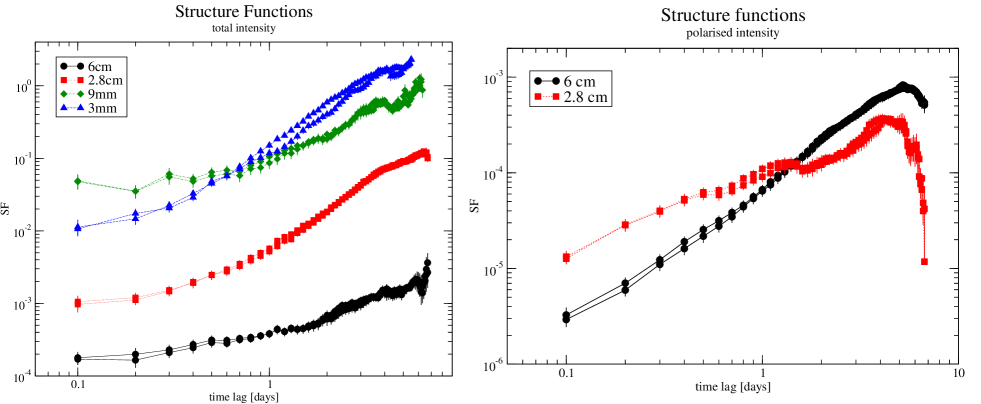
Figure 7: Structure functions of 0716+714 plotted versus time-lag. Different symbols are used for different wavelengths. The panel on the left shows the SF for total intensity, on the right the SF for polarized intensity is shown.

In Fig. 7 we show examples of calculated structure functions for the total and polarized flux density. We note that the error of the derived time scales from the SF and ACF analysis shown in Table 6 is usually high - values of up to 30 % were obtained. The uncertainty of the statistical parameters which quantify the variations in a time series critically depends on the duration of the observation, the sampling interval and the number of significant flux density changes (variability cycles) observed. The light curves of 0716+714 (Fig. 1–6) often show only a monotonic increase and a well defined variability time scale is not observed. This allows only to derive lower limits to the variability time scales (see Appendix B). In the other cases of better defined variability time scales, the measured accuracy is a few 10 %. Here the values obtained by the three different analysis methods are in good agreement.

The prominent and monotonic flux density increase seen at 60, 28, 9 and 3 mm wavelengths appears on similar time scales. The SF analysis yields lower limits of 3.7 to 4.2 days (ACF: 3.0–3.7 days). Due to the lack of pronounced saturation levels in the SFs on time scales $\leq$ 2 days (see Fig. 7), we identify the observed inter-day variability of 0716+714 in total intensity as IDV of type-I according to Heeschen et al. (1987). A significant component of faster variability - with a time scale of $<$ 1 day - was found only at 60mm wavelength. The increasing amplitudes of the SFs shown in Fig. 7 (left), nicely demonstrate the increasing strength of the observed variations towards higher frequencies. The value of the SF at small time lags, $\tau\rightarrow 0$, characterizes the noise level present in the time series. We note that for small time lags ($\tau<0.7$ days), the value of the $\lambda$ 9 mm SF in Fig. 7 (top) is larger than the $\lambda$ 3 mm SF. This can be interpreted with a reduced short time stability of the 9 mm signal, which is affected by the stronger atmospheric influence at the Effelsberg site compared to the high-altitude Pico Veleta site.

Table 6: Variability time scales and lower limits to the variability brightness temperatures for total intensity and polarization in 0716+714. The variability brightness temperatures were derived using Eq. (3).

total intensity
$\lambda$	$t_{SF}$	$\delta t_{SF}$	$T_{B}$	$t_{ACF}$	$\delta t_{ACF}$	$T_{B}$	$\Delta t$	$t_{var}$	$T_{B}$
[mm]	[days]	[days]	[K]	[days]	[days]	[K]	[days]	[days]	[K]
60	0.9	+0.2/–0.2	3.7$\cdot 10^{16}$	0.6	+0.1/–0.1	8.1$\cdot 10^{16}$	–	–	–
	4.2	+0.4/–0.4	2.7$\cdot 10^{15}$	3.1	+0.4/–0.4	4.9$\cdot 10^{15}$	–	–	–
28	$>$ 4.3	+0.3/–0.3	–	$>$ 3.7	+0.2/–0.3	–	4.6	20.9	4.0$\cdot 10^{14}$
9	$>$ 3.7	+0.4/–0.5	–	$>$ 3.2	+0.2/–0.3	–	3.5	10.6	4.2$\cdot 10^{14}$
3.5	$>$ 3.8	+0.1/–0.2	–	$>$ 3.0	+0.2/–0.2	–	4.1	10.7	6.5$\cdot 10^{13}$
linear polarization
60	$>$ 4.5	+0.2/–0.2	–	$>$ 3.2	+0.2/–0.2	–	4.6	8.16	5.6$\cdot 10^{14}$
28	1.3	+0.2/–0.2	2.1$\cdot 10^{15}$	–	–	–	–	–	–
	3.8	+0.3/–0.4	3.2$\cdot 10^{14}$	2.8	+0.5/–0.6	5.6$\cdot 10^{14}$	–	–	–
polarization angle
60	$>$ 6.8	–	–	$>$ 6.8	–	–	–	–	–
28	3.8	+0.1/–0.2	–	3.1	+0.2/–0.2	–	–	–	–

In linear polarization, the source varies at $\lambda$ 60 mm on time scales comparable to those seen in total intensity, whereas at $\lambda$ 28 mm, two variablity time scales are seen: one comparable to the time scale of the total intensity variations ($\sim 4$ days) and a significantly faster component, showing $t_{var}=1.3$ days. The polarization angle changes at $\lambda$ 60 mm display a continuous decrease over the seven days and our analysis yields a lower limit of $t_{var}\geq 6.8$ days. In contrast, the variations of the polarization angle at $\lambda$ 28 mm appear faster by a factor of about two.

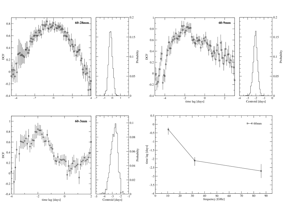
Figure 8: Examples of cross-correlation functions between total intensity light curves obtained at the different frequencies. Here, we show combinations with respect to the data at 60 mm (see top right labels in each plot). The CCPD for the peak of the DCF is shown in the right-hand panels (for details see text). In the bottom right panel, we plot the time lags versus frequency, relative to the light curve at 60 mm. Note the trend of increasing (negative) time lag with increasing frequency.

3.3.2 Variability time scales and brightness temperatures

Assuming that the observed rapid variability would be source intrinsic (see Sect. 4.2), the variability time scales summarized in Table 6 imply very compact emission regions, and hence very high intrinsic brightness temperatures. Following Marscher et al. (1979), and taking an isotropically expanding light-sphere without preferred direction into account, the light travel time argument implies a diameter $d\leq 2\cdot\,c\Delta\,t$ of the emitting region after the time interval $\Delta t$ [s] of expansion. We then obtain for the diameter of the variable emission region $\theta$ [mas]:

$$\theta=0.13\,\frac{t_{var}}{d_{L}}\,\delta(1+z)\,\,,$$ (2)

where $z$ is the redshift of the source, $\delta$ the Doppler factor, $t_{var}$ the logarithmic variability time scale in years (see Appendix B, eq. B5) and $d_{L}$ the luminosity distance in Gpc. Consequently, we find for the brightness temperature $T_{B}$ [K] of a stationary component with a Gaussian brightness distribution (e.g. Kovalev et al., 2005) and flux density $S_{\lambda}$ [Jy]:

$$T_{B}=8.47\times 10^{4}\cdot S_{\lambda}\left(\frac{\lambda\,d_{L}}{t_{var,\lambda}\,(1+z)^{2}}\right)^{2}\,\,.$$ (3)

According to Eq. (3) we calculated the brightness temperatures for the ‘most reliably determined’ variability time scales derived in the previous section (see also Appendix B). Here and in the following we adopt a cosmological distance corresponding to $z=0.3$, which is a lower limit for the redshift of the source (see Sect. 1), and yields a luminosity distance of $d_{L}=1.51$ Gpc assuming a flat universe with $H_{0}=72$ km s^-1 Mpc^-1, $\Omega_{M}=0.3$, $\Omega_{\Lambda}=0.7$ and $\Omega_{k}=0$ (Spergel et al., 2003). In Table 6, we summarize the calculated values of $T_{B}$ for each observing band and for total and polarized intensity, respectively.

For the slow variability of type I seen in the cm-bands, the brightness temperatures range between $4.0\!\cdot\!10^{14}$ K and $4.9\!\cdot\!10^{15}$ K, whereas in the mm-bands, we obtain lower values ranging between $6.5\,\cdot\,10^{13}$ K and $4.2\,\cdot\,10^{14}$ K. The faster type II variability component seen at $\lambda\,60$ mm, leads to a brightness temperature of up to $8.1\,\cdot\,10^{16}$ K, which is at least one order of magnitude higher than the previous estimates. The variations observed in polarized intensity reveal brightness temperatures ranging between $3.2\,\cdot\,10^{14}$ K and $2.1\,\cdot\,10^{15}$ K, similar to those obtained for total intensity in the cm-band. We note that in our calculations we used conservative estimates of the variability time scales, which yield hard lower limits to $T_{B}$. Depending on the assumptions on the geometry and isotropy of the emitting region, the actual brightness temperatures may be higher by a factor of up to 6 (e.g. assuming for the emission region a uniform flat disk of size $d\simeq c\Delta t$ as in the case of a shock). We also note that a larger cosmological distance of 0716+714 would further increase $T_{B}$.

3.4 Cross correlations

To further quantify the close similarities seen in the light curves of 0716+714 across the observing bands, we computed the discrete cross-correlation function (DCF) between different frequencies allowing to search for correlations and possible time lags. We followed the method described by Edelson & Krolik (1988) and Hufnagel & Bregman (1992) for unevenly sampled data, and calculated the DCF and the position of its maximum by using the centroid $\tau_{c}$ of the DCF, given by

$$\tau_{c}=\frac{\sum_{i}{\tau_{i}DCF_{i}}}{\sum_{i}DCF_{i}}\,\,.$$ (4)

In order to obtain statistically meaningful values for the cross-correlation time lags and their related uncertainties, we performed Monte Carlo simulations, following the methods described in detail by Peterson et al. (1998) and Raiteri et al. (2003). Here, we take into account the influence of both uneven sampling and flux density errors. This was done using random subsets of the two data sets. In addition, random Gaussian fluctuations constrained by the measurement errors were added to the flux densities. In each simulation we determined the centroid $\tau_{c}$ of the DCF peak. After running 1000 simulations, we obtained a cross-correlation peak distribution (CCPD), which is shown in the right panel of Fig. 8. This technique yields a reliable measure of the uncertainties in the estimated time lags whereas the values, computed directly from the CCPDs, correspond to 1$\sigma$ errors (see Peterson et al., 1998).

This procedure was applied to each possible frequency combination of the total intensity data (60/28 mm, 60/9 mm, 60/3 mm, 28/9 mm, 28/3 mm, 9/3 mm). Fig. 8 shows some examples of the DCFs and CCPDs relative to the $\lambda\,60$ mm data. Our analysis confirms the existence of a significant correlation across all observed radio-bands. This enables the determination of time lags, which are $\tau_{60/28}\!=\!-0.3^{+0.1}_{-0.3}$ days between the 60 mm and the 28 mm data, $\tau_{60/9}\!=\!-2.1^{+0.2}_{-0.3}$ days between the 60 mm and the 9 mm data, and $\tau_{60/3}\!=\!-2.7^{+0.4}_{-0.4}$ days between the 60 mm and the 3 mm data. This systematic trend is also seen in the time lags relative to the 28 mm data, with $\tau_{28/9}\!=\!-1.9^{+0.2}_{-0.2}$ days and $\tau_{28/3}\!=\!-2.4^{+0.2}_{-0.2}$ days, respectively. In Fig. 8 (bottom right) we plot the $\tau_{60/i}$ time lags for the 3 observing bands ($i=28,9,3$ mm) versus observing frequency. A systematic trend of increasing (negative) time lag towards higher frequencies is evident. This shows that the observed variations (the observed flux density increase) occur first at higher frequencies and then propagate through the radio spectrum towards lower frequencies. The time delay between the two most separated bands ($\lambda\,3$ mm and $\lambda\,60$ mm) is about 2.5 days. This time-lag behavior together with the observed increasing variability amplitudes will be discussed in Sect. 4.

In order to investigate the possible anti-correlation of the total intensity and polarization variations mentioned earlier, we performed a cross-correlation analysis (DCF) also between total and polarized intensity, and between polarized intensity and polarization angle for the 60 and 28 mm wavelengths data. The results are shown in Fig. 9. For both radio bands we confirm an anti-correlation between the total and polarized intensity with a trend of the total intensity leading the polarized intensity by 0.5 days at 60 mm but no obvious time lag at 28 mm. Formally, we also find an anti-correlation between the polarized intensity and polarization angle at 28 mm wavelength.

3.5 Broad-band spectra

In Fig. 10, we show the combined variability data obtained for 0716+714. This multi-frequency data set allows to study the spectral evolution and variability on a daily basis. We construct (quasi-) simultaneous radio spectra using daily averages from the data of all participating radio observatories: Effelsberg, Pico Veleta, SMT/HHT, JCMT, KP and WSRT (see Table 1). The spectral coverage ranges from 1.4 GHz to 666 GHz. At 3 mm wavelength we combined the data from IRAM and KP, to extend the time coverage up to November 17. At 0.8 and 0.85 mm, we used the data from JCMT and the SMT/HHT, which unfortunately do not overlap in time. The time evolution of the cm- to sub-mm spectrum of 0716+714 over the seven observing days (November 11–17; hereafter referred to as days 1 to 7) is presented in Fig. 14. Due to the different duration of the observations at the different telescopes, the maximum frequency coverage was obtained only on day 1 (1.4–666 GHz), whereas for days 6 and 7 the frequency coverage is reduced to 4.85–345 GHz.

0716+714 shows a very inverted radio spectrum over the whole observing period, with small, but significant brightness variations occurring near the spectral turnover during the first five observing days. A pronounced spectral maximum is seen near 90 GHz. Linear fits to the daily spectra yield an averaged spectral slope $\bar{\alpha}_{thick}$ ($S_{\nu}\sim\nu^{\alpha}$) of $+\,0.39\pm 0.02$ for the optically thick part of the spectrum between 1.4 and 86 GHz. Agudo et al. (2006) give for the spectral slope between 86 GHz and 229 GHz a typical $\bar{\alpha}_{86/229}=-0.23\pm 0.10$, a characteristic for the transition towards optical thin synchrotron emission. With the broader frequency coverage shown in Fig. 14, we obtain an average value of $\bar{\alpha}_{thin}=-\,0.30\pm 0.05$. We note that a more detailed analysis of the high frequency data from JCMT indicates that the calibration of the 666 GHz data is uncertain and the measured fluxes come out very low. For this reason we did not include the 666 GHz data in the spectral fitting.

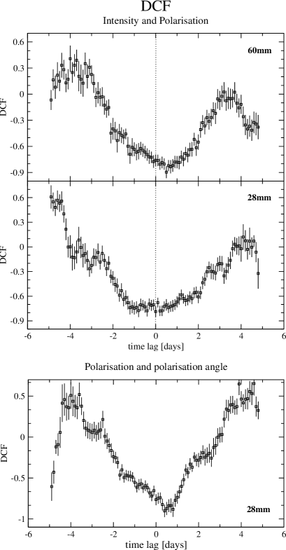
Figure 9: Cross-correlation functions between total intensity and polarization at 60 mm and 28 mm wavelengths. The top panels show the DCFs between total and polarized flux density. The bottom panel shows the DCF for polarized intensity and polarization angle at $\lambda$ 28 mm.

The spectral slopes obtained from the daily fits suggest slight changes with a moderate spectral hardening in the optically thick part (from $\alpha_{thick}=+0.37$ to $\alpha_{thick}=+0.41$ between days 3 and 4) and a spectral steepening in the optical thin part (from $\alpha_{thin}=-0.25$ to $\alpha_{thin}=-0.38$ between days 1 and 3). For the turn-over frequency $\nu_{m}$ we made parabolic fits to the daily spectra, which suggest a small shift of $\nu_{m}$ of about 10 GHz towards lower frequencies. However, these changes in $\alpha$ and $\nu_{m}$ appear not to be statistically significant within our measurement accuracy and the change in frequency coverage of our spectra. A more detailed discussion of the spectrum and its variability will be presented in Sect. 4.3.

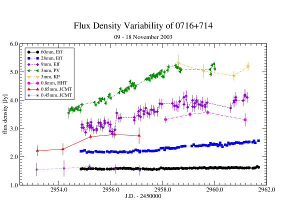
Figure 10: Summary of the total flux density variations in 0716+714 obtained at the various cm- to sub-mm bands during the time of the core campaign. The contribution from each observatory is indicated in the top right insert and in Table 1 (see text for details). For better illustration, the light curve at $\lambda$ 1.3 mm (see Fig. 5), which is affected by larger measurement errors, is not shown.

4 Discussion

4.1 Variability characteristics

4.1.1 Variability in the cm- to mm-regime

During this campaign 0716+714 exhibits very different variability characteristics when compared to previous IDV observations in the cm-regime (e.g. Quirrenbach et al., 1992; Kraus et al., 2003). Usually the source shows rapid IDV on time scales of $\lesssim$ 0.5–1.5 days (in intensity and polarization). In this observation, however, it showed slow inter-day variability on a $\gtrsim$ 3-4 day time scale (total intensity). When 0716+714 exhibits rapid IDV, the variability amplitudes often decreases between 5 and 10 GHz (see Fig. 1 of Krichbaum et al., 2002). A variability amplitude constant or increasing with frequency was observed only occasionally. It is therefore remarkable that this new observations show such a systematic and strong increase of the variability amplitudes (from $Y\!=\!3.7$ % at 5 GHz to $Y\!=\!34$ % at 90 GHz).

A direct comparison with $\lambda$ 60 mm Effelsberg IDV light curves obtained earlier (April 2002) and 8 month later (July 2004) reveal the ‘classical’ IDV behavior, with variability time scales of 0.5–1 days and modulation indices of 2.1–3.4 %. These data sets are shown in Fig. 11 for comparison. This suggests possible changes of the variability characteristics over time scales of weeks to months. We note that a change of the variability time scale from $\sim\,1$ to $\sim\,7$ days was also observed in 0716+714 in 1990 (Quirrenbach et al., 1991; Wagner et al., 1996). Other prominent examples of changes of the variability mode or episodic IDV are PKS 0405$-$385 (Kedziora-Chudczer, 2006) and 0917+624 (Kraus et al., 1999; Fuhrmann et al., 2002, Fuhrmann et al., in prep.).

The good frequency coverage of the observations presented here provides for the first time a possibility to study with dense time sampling the short-term variations from the cm- up to the mm-regime. Here, the correlated variability across all bands, the observed frequency dependence of the variability amplitudes, and the observed time lag with variations at higher frequencies appearing earlier (Sect. 3.4, Fig. 8), argue in favor of a source-intrinsic origin of the observed variations. Such ‘canonical’ variability behavior is usually observed in AGN and other compact radio sources over longer time intervals (weeks to years) and is commonly explained by synchrotron-cooling and adiabatic expansion of a flaring component or a shock (e.g. van der Laan, 1966; Kellermann & Pauliny-Toth, 1968; Marscher & Gear, 1985). In this framework, Raiteri et al. (2003) found similar variability characteristics for the long-term, multi-frequency radio light curves of 0716+714. A possible contribution of scintillation effects and thus extrinsic origin will be discussed in Sect. 4.2. A comparison with the simultaneous optical R-band data presented by Ostorero et al. (2006) will be given in Sect. 4.1.2.

The variability brightness temperatures derived for the total intensity data sets (Table 6, Sect. 3.3.2) reveal lower limits of $4-8\cdot 10^{16}$ K for the faster variability component observed at 60 mm wavelength, and $10^{13.8}-10^{15}$ K for the correlated cm-/mm-wavelength flux density increase on inter-day time scales. We notice a systematic decrease of $T_{B}$ towards higher frequencies. Since $T_{B}$ was derived using the light travel time argument, which implies upper limits to the size of the region of variable emission, it remains uncertain if the observed frequency dependence of the lower limits of $T_{B}$ also reflects a similar frequency dependence of the source-intrinsic brightness temperature. The apparent brightness temperatures, however, exceed the IC limit of $\sim$ 10¹² K (Kellermann & Pauliny-Toth, 1969) by at least $\sim 2$ orders of magnitude, even at mm-wavelengths. If the excessive $T_{B}$ is the result of relativistic aberration, the source radiation must be strongly Doppler-boosted in all of the observed wavebands. The resulting Doppler-factors will be discussed in Sect. 4.4.

From the analysis presented in Sect. 3, we deduce a complex behavior of the polarization variability. We find (i) more pronounced variability amplitudes in polarization than in total intensity (a factor of $\sim$ 15 at $\lambda$ 60 mm), (ii) more pronounced polarization variability (in P and $\chi$) at $\lambda$ 60 mm than at $\lambda$ 28 mm, (iii) significantly faster variability at $\lambda$ 28 mm, and (iv) a clear anti-correlation between total and polarized flux density at both observing bands. Such a complex variability behavior in polarization is often observed in IDV sources (e.g. Kraus et al., 2003), and is interpreted by a multi-component sub-structure of the emitting region(s). The superposition of individually varying and polarized sub-components (characterized by their misaligned polarization vectors) could in principle reproduce the observed polarization variations. At present it is unclear, whether the necessary variability of the individual sub-components is source-intrinsic (e.g. Qian, 1993), solely caused by interstellar scintillation (e.g. Rickett et al., 1995, 2002), or results from a mixture of these effects (Qian et al., 2002). The recent detection of polarization IDV in the VLBI core of 0716+714 clearly places the origin of IDV in the unresolved VLBI core-region, and strongly supports the idea of multiple embedded sub-components of $<100$ $\mu$as size (see Bach et al., 2006). It is unclear, however, whether the different time lags seen between the total and polarized intensity at $\lambda$ 60 mm and $\lambda$ 28 mm have a physical meaning. Source-intrinsic opacity effects and a possible spatial displacement of the polarized sub-components relative to the total intensity component, as often observed for individual jet components with polarization VLBI (e.g. Bach et al., 2006, and references therein), might provide a simple explanation.

Figure 11: IDV light curves of 0716+714 observed with Effelsberg in April 2002 (top) and July 2004 (bottom) at $\lambda$ 60 mm. Note the different and more typical (‘classical’) variability pattern, with faster ($\sim$ 0.5–1 day) and more pronounced $m=2.1\!-\!3.4$ %) variations than those observed in November 2003 (Fig. 1). In the cases shown here, the source was in a fainter radio state than in November 2003, with a mean total flux density of 0.69 and 1.07 Jy in April 2002 and July 2004, respectively.

4.1.2 Long-term variability and broad band characteristics

During the variability campaign in November 2003, 0716+714 was observed in a particular active phase, with a high radio-to-optical state. In fact, between September and October 2003 the source underwent a dramatic and unprecedented outburst in the cm- to mm-bands. In Fig. 12 we show the long-term light curves obtained between 2001 and 2004 at frequencies ranging between 5 and 90 GHz. In addition to the data from this paper, the figure also includes data from the Michigan monitoring (Aller & Aller, private comm.), the Metsähovi blazar monitoring (Teräsranta et al., 2005) and from IRAM (H. Ungerechts, private comm.). Albeit being in the declining phase of the previous large outburst (peak in 2003.8), 0716+714’s flux was rising a second time and was particularly bright in November 2003, reaching more than 5 Jy at 3 mm wavelength. The overall inverted radio-to-mm spectrum during this time indicates a relatively high opacity of the source (synchrotron self-absorption), which is a possible cause for the absence of the usually more pronounced IDV in 0716+714 at the longer cm-wavelengths.

On VLBI scales 0716+714 frequently shows component ejections on time scales of $\sim$ 1–2 years which often are preceeded by larger flux-density outbursts (e.g. Bach et al., 2005). Our daily VLBA observations performed during November 11–16, 2003 (six epochs), however, indicate no strong structural changes at 22 and 43 GHz and on the mas-scale. The flux density of the VLBI core (a $\sim$ 35 % increase from day 1 to 6 at 43 GHz) seems to follow the trend which is seen in the total intensity light curves. A more detailed study of the VLBI results will be presented in a future paper (Agudo et al., in prep.).

During the campaign, 0716+714 was recorded in a moderate level of optical emission in agreement with previous findings, where no obvious strong correlation between prominent radio and optical outbursts have been observed in this source (Raiteri et al., 2003). In the optical R-band, 0716+714 showed intra-night to inter-day variations. The root mean square variability amplitude during the time of the core campaign is $\sim 23$ % (see Fig. 1 in Ostorero et al., 2006). No obvious correlation between the optical and radio variability is seen, indicating that either the emission regions generating radio and optical variability are spatially separated, or the variability in both bands has a different physical origin. We note that also no obvious simultaneous (or delayed) transition of the variability mode is seen between radio and optical, similar to the one reported by Quirrenbach et al. (1991). It is remarkable that during this latter campaign, the source was in a much fainter radio-to-optical state and the radio spectrum (between 5 and 8 GHz) was much less inverted (Wagner et al., 1990; Qian et al., 1996). The presence (or absence) of radio-optical correlations may depend on the source opacity, which is directly related to the observed shape of the radio spectrum and the state of source activity.

Furthermore, we note that in November 2003, 0716+714 was not detected by the INTEGRAL satellite at any of its high energy bands (3-200 keV) and only upper limits to the hard X-ray/$\gamma-$ray emission could be obtained (see Section 4.4.5 and Ostorero et al., 2006). However 0716+714 was seen by INTEGRAL a few months later (at 30-60 keV) (April 2004, Pian et al., 2005), and some flux density variability in the X-ray band was noted.

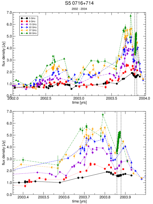
Figure 12: Long-term variability of 0716+714 at 5, 8, 15, 22, 37 and 90 GHz, showing flux densities observed between 2001.5 and 2004 with the Effelsberg, Metsähovi, Michigan and Pico Veleta radio telescopes. The data sets were taken from Teräsranta et al. 2005, Aller & Aller (private comm.), H. Ungerechts (private comm.), and this paper. Note the unusual source brightness during the outburst around 2003.75. The time of the core campaign (November 8-19, 2003) is marked by dashed vertical lines. For better illustration, an enlargement of the variability curves for the time range 2003.45 – 2003.95 is shown in the bottom panel.

4.2 Variability versus frequency: comparison with weak interstellar scintillation

Local scattering in the ISM was clearly demonstrated to be the origin of the most rapid (sub-hour) variability seen in a few IDV sources (e.g. Dennett-Thorpe & de Bruyn, 2001). Further, ISS on longer time scales (days to weeks) is present in a large number of radio sources (e.g. Rickett et al., 2006). Here, we investigate a possible contribution of ISS to the observed cm- up to mm-variability of 0716+714.

In November 2003, 0716+714 varied in a different manner than in previous IDV observations: (i) The observed variability index $m$ at $\lambda$ 60 mm (1.3 %) is (by a factor $\sim$ 2–4) significantly lower than in most earlier experiments (e.g. Quirrenbach et al., 1992; Kraus et al., 2003; Fuhrmann, 2004; Bach et al., 2005). Typically, the variability index peaks around 5 GHz and decreases towards both higher and lower frequencies. This is expected for the transition between weak and strong scattering. The strength of the variability observed in November 2003, however, strongly increases with observing frequency (see Sect. 3 and 4, and Fig. 13). (ii) 0716+714 usually varies fast, on time scales a factor of $\sim$ 2–10 faster than observed here. The prolongation of the variability time scale in November 2003 might be explained as a seasonal effect, caused by the annually changing alignment of the velocity vectors between Earth and scattering screen (as observed for e.g. J1819+3845; Dennett-Thorpe & de Bruyn, 2002). Screen velocities of about 25 km s^-1 w.r.t. the local standard of rest would be sufficient to explain a prolongation in November. However, the multi-frequency time lag (correlation) of the variability pattern, the increase of the modulation index from cm- to mm-bands and the low variability amplitude at $\lambda$ 6 cm are not in agreement with such a scenario. As purely geometric effect, the orbital motion of the Earth’s can affect the variability time scale, but not the strength of the observed variations. We also note that 0716+714 is observed every 4-8 weeks in a regular IDV monitoring project performed with the Urumqi telescope. So far, no strong evidence for annual modulation of the variability pattern is seen (Marchili et al., 2008).

At frequencies of a few GHz, the angular size $\theta$ of an extragalactic self-absorbed, incoherent synchrotron source is usually expected to be larger than the Fresnel scale $\theta_{F}$ for a scattering screen beyond the Solar system (e.g. Beckert et al., 2002). Consequently, we will use a slab-model for weak ISS assuming quenched scattering as described by Beckert et al. (2002). In the regime of weak, quenched scattering ($\theta>\theta_{F}$), the authors give the following analytical solution for the modulation index $m$:

$$m^{2}(\lambda)=2\left(\frac{r_{e}}{D\theta^{2}}\right)^{2}\lambda^{4}(D\theta)^{\beta-2}SM\cdot f_{1}(\beta)\,\,,$$ (5)

with the distance to the scattering screen D, a circular source model with size $\theta$, the scattering measure SM, the power law index $\beta=11/3$ for a Kolmogorov spectrum of density irregularities and the function $f_{1}(\beta)$ of order unity. Depending on the frequency dependence of the source size $\theta$ and for high galactic latitude sources (as 0716+714), the amplitude of the ISS induced variations should thus strongly decrease towards higher frequencies.

Assuming a slab of 1 pc thickness for a thin screen with a strength of turbulence $C_{n}^{2}$, similar to the values derived from pulsar scintillation for enhanced scattering in the Local Bubble (Bhat et al., 1998), we qualitatively compare our multi-frequency results of $m$ directly with ISS according to Eq. (5). Combined Space-VLBI and single-dish observations of 0716+714 place the physical origin of IDV inside the VLBI-core region Bach et al. (2005), which contains about 70 % of the source’s total flux density. Thus, we assume a scintillating component containing 70 % of the observed total flux density, and re-scale the observed modulation indices given in Table 4 according to $m_{70\%}=m/0.7$. In this way, we obtain $m_{70\%}=1.8$ % at $\lambda$ 60 mm, which can be reasonably reproduced by assuming a scintillating source size of 0.25–0.3 mas and and a screen distance of 100–200 pc. Taking these values and assuming a linear dependence of $\theta$ with frequency, we can compare the observed modulation indices at higher frequencies with those expected for weak ISS. The results are shown in Fig. 13. A comparison between observations and model strongly suggests that the ISS model can not reproduce the increasing variability amplitudes observed towards higher frequencies. We obtain similar results by systematically changing the model parameters such as screen distance, source size and scattering measure. Consequently, we conclude that the observed simultaneous and correlated inter-day variations of 0716+714 on time scales of several days in the cm- to mm-band are not strongly affected by scintillation effects, and therefore should be considered as intrinsic to the source.

If ISS dominates the variability at $\lambda$ 60 mm, however, the low variability amplitude and the long variability time scales (compared to previous observations) must indicate strong changes, either in the scattering medium, or in the intrinsic source structure on scales comparable to the scattering size of the medium. Changes in the scattering properties of the screen can be related to either changes in the distance or the strength of turbulence. Both appear unlikely to happen on timescales as short as months. Since 0716+714 was in a flaring state during this observations (see Sect. 4.1), changes in the source structure therefore appear more likely. Flux density outbursts are often accompanied by the ejection of new jet components which, for instance, would temporarily increase the size of the scintillating core region. In such a scenario, the size of the scintillating component should have increased by a factor 2–3 (from about 0.08–0.09 mas to 0.25–0.3 mas) in order to quench $m$, down to the observed level of 1.8 %. The observations performed eight months later (July 2004, Fig. 11) reveal a higher modulation index of $m_{70\%}=3.0$ %, indicating again a smaller scintillating source size of about 0.17–0.19 mas (assuming a screen distance of 100–200 pc). Future VLBI studies with highest possible angular resolution will be needed to relate component ejection, motion and core size evolution with the changes of the IDV pattern in 0716+714.

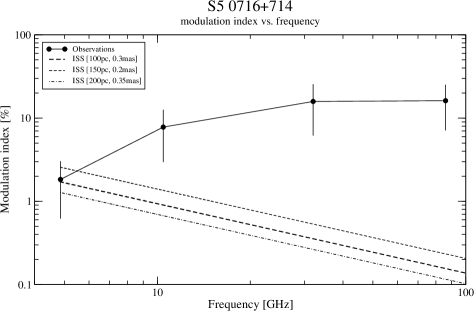
Figure 13: Variability amplitudes of 0716+714 across the observing bands: observed modulation indices versus frequency with ISS model predictions for different parameter ranges (screen distance and source size at $\lambda$ 60 mm) superimposed. Note the strong discrepancy between model calculations and observed values (see text). The statistical errors of $m$ were obtained taking into account the limited total observing time and sampling interval (see Gabányi et al. 2007).

4.3 Synchrotron spectra and spectral evolution

In Fig. 14 we show the evolution of the cm- to sub-mm radio spectra on a daily basis. All spectra are strongly inverted, peaking at $4-5$ Jy near 3 mm wavelength (90 GHz). The results of the spectral fits described in Sect. 3.5 demonstrate that during the whole core campaign the radio spectrum was optically thick up to the mm-band with $\bar{\alpha}_{thick}=+\,0.39\pm 0.02$ and optically thin ($\bar{\alpha}_{thin}=-\,0.30\pm 0.05$) beyond a synchrotron turnover frequency $\nu_{m}$ somewhere close to 90 GHz. This confirms previous findings by Ostorero et al. (2006), who showed the broad band spectral energy distribution (from radio to $\gamma$-rays) using the data of this campaign. The radio spectra shown here (Fig. 14) largely differ from earlier multi-frequency studies, where the source typically showed a flat and only mildly inverted (1 Jy) spectrum (e.g. Chini et al., 1988; Wagner et al., 1990; Quirrenbach et al., 1991). In contrast, the new spectra are indicative of a high peaking and self-absorbed flare spectrum.

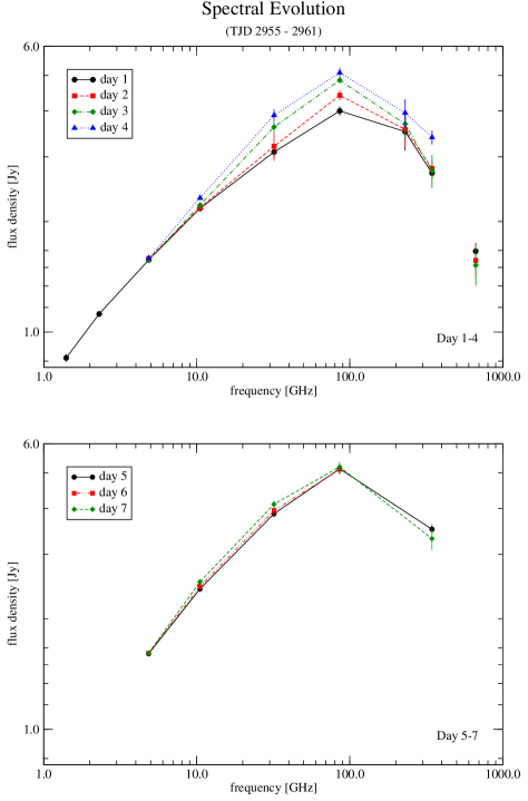
Figure 14: Simultaneous cm- to sub-mm spectra of 0716+714 derived from daily averages of the flux-density measurements shown in Fig. 10. The top-panel shows the spectra for days 1–4 (November 11–14, J.D. $=$ 2452955-58), whereas the spectra of days 5–7 (November 15–17, J.D. $=$ 2452959-61) are shown below. The flux density errors are small and when invisible, comparable or smaller than the size of the symbols.

Significant changes in the cm- to sub-mm spectra occur mainly until day 5, i.e. during the period of the monotonic increase in total flux density seen across all bands. Here, the spectral peak flux increases, reaching its maximum on day 5. The daily averaged peak flux density (at $\nu_{m}$) rises from $S_{86\,GHz}=4.0$ Jy on day 1 to $S_{86\,GHz}=5.1$ Jy on day 5. After this date, no further changes are evident (see also Fig. 10).

The absence of pronounced variations in the spectral slopes and the turnover frequency (achromatic variations) would indicate a geometrical origin, i.e. caused by changes in the beaming factor (e.g. in a helical/precessing jet; Begelman et al., 1980; Villata & Raiteri, 1999). The possible slight changes in the daily spectral slopes (spectral steepening for $\nu\,<\,\nu_{m}$, the spectral softening for $\nu\,>\,\nu_{m}$) and marginal shift of the turn-over frequency towards lower energies ($\Delta\nu\sim 10$ GHz), suggest that the spectral evolution is not fully achromatic. The limited time coverage (only 7 days) prevents a more detailed analysis of the spectral evolution. However, the presence of source intrinsic spectral variations is also supported by the canonical behavior of the time lag (discussed in Sect. 3.4) and the related frequency dependence of the variability amplitudes, which increase towards the mm-bands. Therefore, an interpretation within standard flare/adiabatic expansion and/or shock-in-jet models appears applicable (e.g. Marscher & Gear, 1985).

The optically thick spectral index, however, strongly differs from the canonical value for a self-absorbed, homogeneous synchrotron component ($S_{\nu}\sim\nu^{5/2}$). This indicates that the flaring component, which dominates the observed radio-spectrum, is inhomogeneous and may consists of more homogeneous but smaller sub-components, peaking at slightly different self-absorption frequencies (see also Ostorero et al., 2006). This view is further supported by (non-simultaneous) mm-VLBI observations of 0716+714, which indeed show multiple components on the 0.05 - 0.1 mas scale (T. Krichbaum, unpublished data).

4.4 Doppler factors and magnetic field

In this section we will compare the Doppler factors $\delta_{var}$ deduced from the variability brightness temperatures of Sect. 3.3.2 with Doppler factors calculated by other methods. In particular, we will compare $\delta_{var}$ with (i) estimates derived from VLBI studies of 0716+714 ($\delta_{VLBI}$), (ii) the equipartition Doppler factor $\delta_{eq}$, using calculations of the synchrotron and equipartition magnetic field, (iii) $\delta_{var,eq}$ using the equipartition brightness temperature $T_{eq}$, and (iv) the inverse Compton Doppler factor $\delta_{IC}$ as calculated from the simultaneous INTEGRAL observations.

4.4.1 Doppler factor $\delta_{var,IC}$

The limits of the apparent brightness temperature ($T_{B}^{app}$) summarized in Table 6 exceed by several orders of magnitude the IC-limit of $T_{B,IC}^{lim}\sim$ 10¹² K (Kellermann & Pauliny-Toth, 1969). In order to explain the excessive temperatures solely by relativistic boosting of the radiation, source intrinsic radiation near the IC-limit can be assumed ($T_{B}=T_{B,IC}^{lim}$), which leads to a lower limit to the Doppler factor of the emitting region of $\delta_{var,IC}=(1+z)\sqrt[3+\alpha]{T_{B}^{app}/10^{12}}$. This leads to Doppler factors $\delta_{var,cm}>$ 10–22 in the cm-regime and $\delta_{var,mm}>$ 5–10 in the mm-regime (assuming z $=$ 0.3), which lower the observed brightness temperatures of Table 6 down to the IC-limit. In the case of the faster variability component seen at $\lambda\,60$ mm, the situation becomes more extreme. Here, Doppler factors $\delta_{var,IC}$ $>$ 43 would be needed if, again, sole intrinsic in origin. Although high, these limits for $\delta_{var,cm}$ and $\delta_{var,mm}$ agree well with recent estimates coming from kinematic VLBI studies of the source. From 26 epochs of VLBI data observed between 1992 and 2001, Bach et al. (2005) found atypically high superluminal motion and conclude that the minimum Doppler factor is $\delta_{VLBI}\geq$ 20–30, assuming a redshift of $z\geq 0.3$. This confirms the previously reported high speeds (16–21 c) in 0716+714 (Jorstad et al., 2001). Moreover, using a larger sample of sources, Jorstad et al. (2005) observed $\delta_{VLBI}>$ 16–21 in 9 of the 13 studied blazar indicating that strong Doppler boosting is not a rare phenomenon in compact VLBI jets.

We further note that the observed decrease of $T_{B}^{app}$ towards higher frequencies suggests that the Doppler factors at cm- and mm-wavelengths could be different. This appears not unlikely in a model of a stratified and optically thick self-absorbed bent jet, where at each wavelength spatially different jet regions are probed. Each of these regions may exhibit characteristic Doppler factors depending on jet speed and viewing angle. As one looks at higher frequencies into regions which are deeper embedded in the source, a lower brightness temperature and resulting lower $\delta_{var}$ towards the innermost jet regions would then indicate either jet-acceleration (changes of the Lorenz factor along the jet) and/or jet bending with changes of the jet orientation away from the observer‘s line of sight for outward oriented motion.

4.4.2 Magnetic field from synchrotron self-absorption

Using standard synchrotron expressions, it is possible to constrain the magnetic field B in 0716+714 by means of the spectral parameters deduced in the previous section. Assuming a homogenous synchrotron self-absorbed region, a closed expression for B is given by (see e.g. Marscher, 1987)

$$B_{SA}\,[G]\,=10^{-5}b(\alpha)\theta^{4}\nu_{m}^{5}S_{m}^{-2}\left(\frac{\delta}{1+z}\right),$$ (6)

with the tabulated quantity b$(\alpha)$ depending on the optically thin spectral index $\alpha_{thin}$ (see Table 1 in Marscher, 1987), the flux density $S_{m}$, the source angular size $\theta$ at the synchrotron turnover frequency $\nu_{m}$ and the Doppler factor $\delta$. At $\nu_{m}=86$ GHz, the size of the emitting region responsible for the observed variations can be constrained using recent mm-VLBI measurements of the core region of 0716+714 (Bach et al., 2006; Agudo et al., 2006) which yield $\theta_{86\,GHz}<0.04$ mas. Using the observed spectral parameters from above ($S_{86\,GHz}\!=\!4.0-5.13$ Jy, $\bar{\alpha}_{thin}\!=\!-\,0.30$,) we calculate a lower limit of the magnetic field $B_{SA}$ in the range of $0.07-0.11\,\delta\,$G for $\nu_{m}\!=\!86$ GHz without correcting for Doppler boosting.

4.4.3 Magnetic field from equipartition

The magnetic field $B_{SA}$ calculated according to Eq. (6) can be used to constrain the Doppler factor in an alternative way. The magnetic equipartition field $B_{eq}$, which minimizes the total energy $E_{tot}=(1+k)E_{e}+E_{B}$ (with relativistic particle energy $E_{e}\sim B^{-1.5}$ and energy of the magnetic field $E_{B}\sim B^{2}$), is given by the following expression (e.g. Pacholczyk, 1970; Bach et al., 2005):

$$B_{eq} = \left(4.5\cdot(1+k)\,f(\alpha,\nu_{a},\nu_{b})\,L\,R^{3}\right)^{2/7}$$ (7)

$$= 1.65\cdot 10^{10}\left(f(\alpha,\nu_{a},\nu_{b})\,(1+z)\,S_{m}\,\nu_{m}\,d_{L}^{2}\,R^{-3}\right)^{2/7}$$

with the energy ratio $k$ between electrons and heavy particles, the synchrotron luminosity $L=4\pi\,d_{L}^{2}(1+z)\int^{\nu_{a}}_{\nu_{b}}{S\,d\nu}$ of the source, the size of the component R in cm, $S_{m}$ and $\nu_{m}$ in GHz and the tabulated function $f(\alpha,\nu_{a},\nu_{b})$ with the upper and lower synchrotron frequency cutoffs $\nu_{a},\nu_{b}$. Using $\nu_{a}=10^{7}$ Hz, $\nu_{b}=5.5\cdot 10^{14}$ Hz (e.g. Biermann & Strittmatter, 1987; Ghisellini et al., 1993), $k\approx 100$ and the same values as for Eq. (6), we calculate a lower limit for the magnetic field in the range of 1.2–1.3 G, which is higher than the magnetic field obtained in the previous section. Eq. (6) and (7) give different dependencies of $B$ and $\delta$: $B_{SA}\sim\delta$, $B_{eq}\sim\delta^{2/7\alpha+1}$. This yields $B_{eq}/B_{SA}=\delta_{eq}^{2/7\alpha}$. Adopting the above numbers, we obtain Doppler factors $\delta_{eq}$ in the range of 12–23, in good agreement with both, the previous estimates for $\delta_{var}$ as well as $\delta_{VLBI}$.

4.4.4 Equipartition brightness temperature $T_{B,eq}^{lim}$

Instead of using the IC limit of $10^{12}$ K for the intrinsic brightness temperature, a brightness temperature limit based on equipartition between particle energy and field energy could be used (Scott & Readhead, 1977; Readhead, 1994): $T_{B,eq}\sim\,3\cdot 10^{11}$ K. It is argued that this limit better reflects the stationary state of a synchrotron source and for many sources is $\lesssim\,10^{11}$ K (e.g. Readhead, 1994; Guijosa & Daly, 1996). With these numbers we obtain another estimate of the Doppler factor: $\delta_{var,eq}=(1+z)\sqrt[3+\alpha]{T_{B}^{app}/3\cdot 10^{11}}>$ 8–33, where we again used $T_{B}^{app}$ from Table 6. Although high, these values still agree with the previous estimates and also with $\delta_{VLBI}$.

4.4.5 Inverse Compton Doppler factor $\delta_{IC}$

Finally we can independently calculate the Doppler factor $\delta_{IC}$ using the upper limits to the soft $\gamma$-ray flux densities of 0716+714 obtained from the INTEGRAL observations during this experiment and the inverse Compton argument (see also Ostorero et al., 2006; Agudo et al., 2006). Following (see e.g. Marscher, 1987; Ghisellini et al., 1993) the IC Doppler factor $\delta_{IC}$ is calculated from:

$$\delta_{IC}=f(\alpha)S_{m}\left(\frac{ln(\nu_{b}/\nu_{m})\nu_{\gamma}^{\alpha}}{S_{\gamma}\theta_{\nu}^{(6-4\alpha)}\nu_{m}^{(5-3\alpha)}}\right)^{1/(4-2\alpha)}(1+z)\,\,.$$ (8)

where $\nu_{b}$ is the synchrotron high frequency cut-off in GHz, $S_{m}$ the flux density in Jy at the synchrotron turnover frequency $\nu_{m}$, $S_{\gamma}$ the observed $\gamma$-ray flux in Jy at $\nu_{\gamma}$ in keV, $\theta$ the source angular size in mas and a function of spectral index $f(\alpha)\simeq 0.14-0.08\alpha$ (e.g. Ghisellini et al., 1993). If we determine the size $\theta_{\nu}$ via the causality argument and with the variability time scale $t_{var}$, an additional $\delta$ comes in Eq. (2) (see also Agudo et al., 2006) and we can rewrite Eq. (8):

$$\delta_{IC}=\left[f(\alpha)S_{m}(1+z)\right]^{(4-2\alpha)/(10-6\alpha)}\left(\frac{ln(\nu_{b}/\nu_{m})\nu_{\gamma}^{\alpha}}{S_{\gamma}\theta^{(6-4\alpha)}\nu_{m}^{(5-3\alpha)}}\right)^{1/(10-6\alpha)}\,\,.$$ (9)

whereas now the apparent variability size is calculated from $\theta\equiv 0.13\,t_{var}d_{L}^{-1}\,(1+z)$. Using the same values for $\nu_{m}$, $\nu_{b}$, $\alpha_{thin}$ as above and $S_{86\,GHz}\!=\!5.13$ Jy, $t_{var}=10.7$ days (Table 6), we calculate $\delta_{IC}$ using the upper limits to the soft $\gamma$-ray flux in the four bands of INTEGRAL (8, 23, 63 and 141 keV, see also Ostorero et al., 2006). The upper limits to the $\gamma$-ray flux lead to lower limits to the IC Doppler-factors, which for the different energy bands are summarized in Table 7. As outlined by Agudo et al. (2006), the lower limit of $\delta_{IC}\!>\!14.1$ obtained in this way provides a more robust constraint on the Doppler factor than $\delta_{var}$ and $\delta_{eq}$ due to the weak dependence of Eq. (9) on z and $d_{L}$ for $\alpha_{thin}\!=\!-0.3$. We further note that the values of $\delta_{IC}\!>\!14$ obtained here are in very good agreement with a Doppler factor of $\delta\,\sim\,17$ derived by Tagliaferri et al. (2003), who fit the SEDs of 0716+714 by a homogenous, one-zone synchrotron/inverse Compton model.

Table 7: Summary of the Doppler factor estimates using the different methods presented in Sect. 4.4. See text for details.

$\delta$	value	used values/quantities
$\delta_{var,IC,cm}$	$>$ 10–22	$T_{B}^{app}$ (Table 6), $T_{B,IC}^{lim}=$ 1012 K
$\delta_{var,IC,mm}$	$>$  5–10	$T_{B}^{app}$ (Table 6), $T_{B,IC}^{lim}=$ 1012 K
$\delta_{var,eq}$	$>$  8–33	$T_{B}^{app}$ (Table 6), $T_{B,eq}^{lim}=\,3\cdot 10^{11}$ K
$\delta_{eq}$	$>$ 12–23	$B_{SA}$, $B_{eq}$, $S_{86\,GHz}\!=\!4.0-5.13$ Jy,
		$\alpha_{thin}\!=\!-0.3$, $\theta_{VLBI}<0.04$ mas
$\delta_{IC,8\,keV}$	$>$ 15.9	$S_{8\,keV}=1.37\cdot 10^{-7}$ Jy, $\alpha_{thin}\!=\!-0.3$
		$S_{86\,GHz}\!=\!5.13$ Jy, $t_{var}=10.7$ days
$\delta_{IC,23\,keV}$	$>$ 14.7	$S_{23\,keV}=2.55\cdot 10^{-7}$ Jy, $\alpha_{thin}\!=\!-0.3$
		$S_{86\,GHz}\!=\!5.13$ Jy, $t_{var}=10.7$ days
$\delta_{IC,63\,keV}$	$>$ 15.3	$S_{63\,keV}=1.23\cdot 10^{-7}$ Jy, $\alpha_{thin}\!=\!-0.3$
		$S_{86\,GHz}\!=\!5.13$ Jy, $t_{var}=10.7$ days
$\delta_{IC,141\,keV}$	$>$ 14.1	$S_{141\,keV}=2.42\cdot 10^{-7}$ Jy, $\alpha_{thin}\!=\!-0.3$
		$S_{86\,GHz}\!=\!5.13$ Jy, $t_{var}=10.7$ days

In Table 7 we summarize the Doppler-factors $\delta$ calculated using the different methods presented above. A comparison of the numbers shows a general good agreement with the Doppler factor $\delta_{VLBI}$ derived from the superluminal VLBI kinematics. Although strong Doppler boosting is required, these values appear to be not excessively high, and therefore provide a self-consistent explanation of the high apparent variability brightness temperatures, without a violation of the theoretical limits. Since no excessive $\gamma-$ray emission and therefore no IC catastrophe was recorded by INTEGRAL, and a strong contribution of ISS is unlikely, we thus conclude that the violation of the theoretical limits inferred from our observations was only apparent and intrinsic Doppler boosting can naturally explain the non-detection of the source at high energies. However, we stress that all derived values of $\delta$ must be regarded as lower limits. Consequently, Doppler-factors much higher than $\delta>20-30$ can still not be ruled out completely. Contributions from other radiation processes, such as partially coherent emission, can not be ruled out either.

5 Summary and Conclusions

We presented the results of a combined variability analysis from an intensive multi-frequency campaign on the BL Lac 0716+714 performed during seven days in November 2003. From seven participating radio observatories we obtain a frequency coverage of 1.4–666 GHz. Densely sampled IntraDay Variability (IDV) light curves obtained at wavelengths of 60, 28, 9, 3, and 1.3 mm allowed for the first time a detailed analysis of the source’s intra- to inter-day variability behavior over the full radio- to short mm-band. In this observing campaign 0716+714 was found to be in a particular slow mode of variability, when compared to all previous IDV observations of this source. While in total intensity a component of faster variability was observed only at $\lambda$ 60 mm, the source’s flux density in the cm- to mm-regime was dominated by a nearly monotonic increase on inter-day time scales and with variability amplitudes strongly increasing towards higher frequencies. Here, our CCF analysis confirms that the flux density variations are correlated across the observing bands, with variability at shorter wavelengths leading. This and the observed frequency dependence, which cannot be explained by a model for weak scintillation, strongly suggest that the observed inter-day variability has to be considered as source-intrinsic rather than being induced by ISS. Only at 60 mm wavelength a component of faster variability is seen and implies an unusually high apparent brightness temperature $T_{B}$. Hence, ISS might be present at this frequency.

The non-detection of the ‘classical’, more rapid (type II) IDV behavior of 0716+714 in the cm-bands is most likely caused by opacity effects and can be related to the overall flaring activity of the source shortly before and during this campaign. Since episodic IDV behavior is also observed in other sources (e.g. Fuhrmann et al., 2002; Kedziora-Chudczer, 2006), it appears likely that the variability pattern in ‘classical’ type II IDV sources is strongly affected by the evolution of their intrinsic complex structure on time scales of weeks to months. The observed complicated variability patterns in total intensity and polarization, and their correlations, indicate the existence of a multi-component structure with individually varying and polarized sub-components of different size.

From daily averages, the spectral evolution of the highly inverted radio-to-sub-mm spectrum of 0716+714 could be studied. During the seven observing days the spectrum always peaked near $\nu_{m}\!\sim\!86$ GHz. Significant changes of the peak flux mainly occurred during the first 5 days with a continuous rise of the peak flux density from 4 to 5 Jy. Together with possibly small changes in the daily spectral slopes and the peak frequency $\nu_{m}$, the observed variations follow the ‘canonical’ behavior and indicate time-variable synchrotron self-absorption and adiabatic expansion of a shock or a flaring component as described by standard models (e.g. Marscher & Gear, 1985).

The apparent brightness temperatures $T_{B}$ obtained from the inter-day variations exceed theoretical limits by several orders of magnitudes. Although $T_{B}$ decreases towards the mm-bands, the $10^{12}$ K IC-limit is always violated. Assuming relativistic boosting of the radiation, the source must always be strongly Doppler boosted. We obtain lower limits to the Doppler factor of the source using different methods, including (i) inverse Compton ($\delta_{var,IC}$) and equipartition ($\delta_{var,eq}$) estimates using the variability brightness temperatures, (ii) an estimate $\delta_{eq}$ using calculations of the synchrotron and equipartition magnetic field, and (iii) an inverse Compton Doppler factor $\delta_{IC}$ using the data from the simultaneous INTEGRAL observations. These methods reveal robust and self-consistent lower limits to the Doppler factor with $\delta_{var,IC}>$ 5, $\delta_{var,eq}>$ 8 and $\delta_{eq}>$ 12. These limits are in good agreement with estimates based on recent kinematical VLBI studies of the source and the IC Doppler factor $\delta_{IC}>$ 14 obtained from the upper limits to the high energy emission in the 3–200 keV bands. The non-detection of the source in the soft $\gamma$-ray bands implies the absence of a simultaneous strong IC catastrophe during the period of our IDV observations. Since a strong contribution of interstellar scintillation to the observed inter-day variability can be excluded, we conclude that relativistic Doppler boosting appears to naturally explain the observed apparent violation of the theoretical brightness temperature limits.

Appendix A Statistical variability analysis

As a criterion for the presence of variability, the hypothesis of a constant function (non-variable source) is examined and a $\chi^{2}$-test of the variability curve $S_{i}$ is done:

$$\chi^{2}=\sum_{i=1}^{N}\left(\frac{S_{i}-<S>}{\Delta S_{i}}\right)^{2}\,\,,$$ (10)

with the reduced $\chi_{r}^{2}$

$$\chi_{r}^{2}=\frac{1}{N-1}\sum_{i=1}^{N}\left(\frac{S_{i}-<S>}{\Delta S_{i}}\right)^{2}\,\,.$$ (11)

Here, $S_{i}$ denotes the individual flux density measurements at time $i$, $<S>$ their average in time, $\Delta S_{i}$ the individual measurement errors and N the number of measurements (e.g. Taylor, 1982; Bevington & Robinson, 1992). A source is considered to be variable if the $\chi^{2}$-test gives a probability of $\leq 0.1\,\%$ for the assumption of constant flux density (99.9 % significance level for variability).

To further quantify the observed variability, the modulation index $m$ is calculated. This quantity provides a useful measure of the strength of the observed variations and is defined as the percentage ratio of the rms-fluctuations $\sigma_{S}$ of the time series and the time averaged mean flux density $<S>$:

$$m[\%]=100\cdot\frac{\sigma_{S}}{<S>}\,\,.$$ (12)

In order to take the residual calibration errors into account, we follow Heeschen et al. (1987) and calculate the variability amplitude $Y$ for each individual light curve:

$$Y[\%]=3\sqrt{m^{2}-m_{0}^{2}}\,\,.$$ (13)

The $Y$-amplitude can be regarded as being equivalent to a noise-bias corrected variability amplitude using the mean modulation index $m_{0}$ of the secondary calibrators as a measure of the overall calibration accuracy.

A similar analysis was performed for polarization. The corresponding quantities for Polaris ed intensity $S_{P}$ are

$$m_{P}[\%]=100\cdot\frac{\sigma_{S_{P}}}{<S_{P}>}\,\,,$$ (14)

$$Y_{P}[\%]=3\sqrt{m_{P}^{2}-m_{P,0}^{2}}\,\,.$$ (15)

For the the polarization angle $\chi$ we use

$$m_{\chi}[^{\circ}]=\sigma_{\chi}\,\,,$$ (16)

$$Y_{\chi}[^{\circ}]=3\sqrt{\sigma_{\chi}^{2}-\sigma_{\chi,0}^{2}}\,\,.$$ (17)

A $\chi^{2}$-test for $S_{P}$ and $\chi$ was performed similar to total intensity, i.e. using Eq. (10) and (11).

Appendix B Variability time scales

(i) Structure function analysis

Following Heeschen et al. (1987) and Kraus et al. (1999), the time series were analyzed by first order structure functions (SF). The following procedure was used and applied to each data set in order to obtain a variability time scale at every frequency (see also Beckert et al., 2002). For each data set $f(t_{i})$, the discrete structure function

$$SF(\tau_{j}) = N^{-1}_{ij}\sum_{i=1}^{n}w(i)w(i+j)[f(t_{i})-f(t_{i}+\tau_{j})]^{2}$$ (18)

was calculated. Here, $N_{ij}$ is the normalization, $t_{i}$ and $t_{i}+\tau_{j}$ are the times at which the flux densities $f$ were obtained, and $w(i)$ and $w(i+j)$ are weighting functions with $w(i)w(i+j)>0$. The weighting function accounts for binning of an unevenly sampled time series. The binning interval was chosen to be $\sim$ 3–5 times of the typical sampling interval of the light curve. In addition, the structure functions were also calculated using an interpolation method similar to that described by Edelson & Krolik (1988). This showed no significant differences in the results compared to the discrete method. Subsequently, two linear fits were performed to estimate the slope of the SF ($SF=a\cdot\tau^{\beta}$) and the plateau level ($\rho_{0}=2m^{2}$). This plateau (or saturation) level is determined through calculation of the mean value of the SF after the first maximum, the related error by the variance of the mean value. The formal error of the power law fit to the SF is determined by the variance of the fit parameters $a$ and $\beta$. The variability time scale is then determined by the crossing point of the power law and the fitted saturation level, $\rho_{0}=a\cdot t^{\beta}$, and is given by

$$t_{SF}=\left(\frac{\rho_{0}}{a}\right)^{1/\beta}\,\,,$$ (19)

with its formal error

$$\Delta t_{SF}=\left(\frac{\rho_{0}\pm\Delta\rho_{0}/\sqrt{3}}{a\pm\Delta a/\sqrt{3}}\right)^{\frac{1}{\beta\pm\Delta\beta/\sqrt{3}}}\,.$$ (20)

In case of no clear saturation of the SF during the whole observing period, only a lower limit to the variability time scale is given (Table 6, columns 2 and 3).

(ii) Auto-correlation function analysis

In the investigation of pulsar scintillation, the usual way is to define the “de-correlation” time scale as the time lag during which the auto-correlation function (ACF) falls to 1/e of its maximum (e.g. Cordes, 1986). The auto-correlation function $\rho(\tau)$ of a time series $S(t_{i})$ is defined as (Edelson & Krolik, 1988)

$$\rho(\tau)=<(S(t)\cdot S(t-\tau))>_{t}\,\,.$$ (21)

The ACF was calculated and $t_{ACF}$ was determined by the full-width of the ACF at 1/e-height of its maximum. This method was applied to our data sets in total intensity and polarization. The error estimations were obtained taking the individual uncertainties of the calculated auto-correlation functions into account. Columns 5 and 6 of Table 6 summarize the resulting characteristic time scales and error estimates.

(iii) Minimum-maximum method

The observed total intensity variability patterns are mainly characterized by a quasi-monotonic increase of the flux density over a significant range of the total observing period. Consequently the SF/ACF methods deliver variability time scale of $3-4$ days, which owing to the limited total observing time must formally be regarded as lower limits to the true variability time scale $t_{var}$. In these cases we make use of the following definition of the time scale $t_{var}$ to obtain better estimates of the “true” variability time scales directly from those time series where only a several day trend was observed (see also Marscher et al., 1979, and references therein):

$$t_{var}=\arrowvert\frac{dln\,S}{dt}\,\arrowvert^{-1}=\frac{<S>\,\Delta t}{\Delta S}\,\,,$$ (22)

where $<S>$ denotes the mean flux density [Jy] and $\Delta S=S_{max}-S_{min}$ the flux density variation in the considered time interval $\Delta t$.

We note that this time scale relies on a ‘visual’ inspection of the variability curves, defining by human eye (or mathematically via differentiation) the minimum and maximum of the flux density and the corresponding time interval $\Delta t$ between these two flux density levels. In Table 6, columns 8 & 9 summarize the derived values for $\Delta t$ and $t_{var}$ of Eq. (22).