Non-equilibrium self-assembly of a filament coupled to ATP/GTP hydrolysis

Abstract

We study the stochastic dynamics of growth and shrinkage of single actin filaments or microtubules taking into account insertion, removal, and ATP/GTP hydrolysis of subunits. The resulting phase diagram contains three different phases: a rapidly growing phase, an intermediate phase and a bound phase. We analyze all these phases, with an emphasis on the bound phase. We also discuss how hydrolysis affects force-velocity curves. The bound phase shows features of dynamic instability, which we characterize in terms of the time needed for the ATP/GTP cap to disappear as well as the time needed for the filament to reach a length of zero (i.e. to collapse) for the first time. We obtain exact expressions for all these quantities, which we test using Monte Carlo simulations.

Key words: Actin; Microtubule; Dynamic instability; ATP hydrolysis; Force-velocity curves; Stochastic dynamics

Introduction

A large number of structural elements of cells are made of fibers. Well studied examples of these fibers are microtubules and actin filaments. Microtubules are able to undergo rapid dynamic transitions between growth (polymerization) and decay (depolymerization) in a process called dynamic instability (1). Actin filaments are able to undergo treadmilling-like motion. These dynamic features of microtubules and actin filaments play an essential role in cellular biology (2). For instance, the treadmilling of actin filaments occurs in filopodia, lamellipodia, flagella and stereocilia (3, 4, 5). Actin growth dynamics is also important in acrosome reactions, where sperm fuses with egg (6, 7, 8). During cell division, the movements of chromosomes are coupled to the elongation and shortening of the microtubules to which they bind (9, 2).

Energy dissipation is critical for these dynamic non-equilibrium features of microtubules and actin. Energy is dissipated when ATP (respectively GTP) associated to actin monomers (respectively tubulin dimers) is irreversibly hydrolyzed into ADP (respectively GDP). Since this hydrolysis process typically lags behind the assembly process, a cap of consecutive ATP/GTP subunits can form at the end of the filament (10, 11).

Let us first consider studies of the dynamic instability of microtubules. Non-equilibrium properties of microtubules have often been described using a phenomenological two-state model developed by Dogterom and Leibler (12). In such a model, a microtubule exists either in a rescue phase (where a GTP cap exists at the end of the microtubule) or a catastrophe phase (with no GTP cap), with stochastic transitions between the two states. A limitation of such a model is that a switching frequency is built in the model rather than derived from a precise theoretical modeling of the GTP cap. This question was addressed later by Flyvbjerg et al. (13, 14), where a theory for the dynamics of the GTP cap was included. At about the same time, a mathematical analysis of the Dogterom-Leibler model using Green functions formalism was carried out in ref. (15). The study of Flyvbjerg et al. (13, 14), was generalized in (16), with the use of a variational method and numerical simulations. This kind of stochastic model for the dynamic instability of microtubules was further studied by Antal et al. (17, 18). The Antal et al. model takes into account the addition and hydrolysis of GTP subunits, and the removal of GDP subunits. Exact calculations are carried out in some particular cases such as when the GDP detachment rate goes to zero or infinity, however no exact solution of the model is given for arbitrary attachment and detachment rates of both GTP and GDP subunits.

It was thought for a long time that only microtubules were able to undergo dynamic instability. Recent experiments on single actin filaments, however, have shown that an actin filament can also have dynamic-instability-like large length fluctuations (19, 20). A similar behavior was observed in experiments where actin polymerization was regulated by binding proteins such as ADF/Cofilin (21, 22). Vavylonis et al. (23) have studied theoretically actin polymerization kinetics in the absence of binding proteins. Their model takes into account polymerization, depolymerization and random ATP hydrolysis. In their work, the ATP hydrolysis was separated into two steps: the formation of ADP-Pi-actin and the formation of ADP-actin by releasing the phosphate Pi. Vavylonis et al. have reported large fluctuations near the critical concentration, where the growth rate of the filament vanishes. More recently Stukalin et al. (24) have studied another model for actin polymerization, which takes into account ATP hydrolysis in a single step (neglecting the ADP-Pi-actin state) and occurring only at the interface between ATP-actin and ADP-actin (vectorial model) or at a random location (random model). This model too shows large fluctuations near the critical concentration, despite the differences mentioned above. Note that both mechanisms (vectorial or random) are still considered since experiments are presently not able to resolve the cap structure of either microtubule or actin filaments.

In this paper, we study the dynamics of a single filament, which can be either an actin filament or a microtubule, using simple rules for the chemical reactions occurring at each site of the filament. The advantage of such a simple coarse-grained non-equilibrium model is that it provides insights into the general phenomenon of self-assembly of linear fibers. Here, we follow the model for the growth of an actin filament developed in ref. (24). We describe a new dynamical phase of this model, which we call the bound phase by analogy with two-state models of microtubules (12). The characterization of this bound phase is particularly important, because experimental observations of time-independent filament distribution of actin or microtubules (19) are likely to correspond to this phase. In addition, we analyze the dynamic instability with this model. We think that dynamic instability is not a specific feature of microtubules but could also be present in actin filaments. We argue that one reason why dynamic instability is less often observed with actin than with microtubules has to do with the physical values of some parameters which are less favorable for actin than for microtubules. This conclusion is also supported by the work of Hill in his theoretical study of actin polymerization (10, 11). In these references, a discrete site-based model for a single actin filament with the vectorial process of hydrolysis is developed, which has many similarities with our model.

In short, the model studied in this paper presents three dynamical phases, which are all non-equilibrium steady states: a bound phase (phase I), where the average cap length and the filament length remain constant with time, an intermediate phase (phase II), where the average cap length remains constant and the filament grows linearly with time, and a rapidly growing phase (phase III) where the cap and the filament both grow linearly with time. The phases II and III were already present in the study of ref. (24), but phase I was not analyzed there. Thus the description of the main features of phase I (such as the average length, the distribution of lengths) is one of main results of this paper.

In addition, we discuss how GTP/ATP hydrolysis affects force-velocity curves and we characterize the large fluctuations of the filament, by calculating the time needed for the cap to disappear in phase I and II as well as the time needed for the complete filament to reach a length of zero (i.e. to collapse) for the first time in phase I. Due to the simplicity of the model, we are able to obtain exact expressions for all these quantities. We also test these results using Monte Carlo simulations.

Model

We study a model for the dynamics of of single actin or microtubule filaments taking into account ATP/GTP hydrolysis. Our model is very much in the same spirit as that of ref. (24) and has also several common features with the Hill et al. model (10, 11). We assume that polymerization occurs, for actin, via the addition of single ATP subunit (GTP subunit for microtubule), at the barbed end (plus end for microtubule) (2) of the filament. We assume that the other end is attached to a wall and no activity happens there. Let $U$ and $W_{T}$ be the rates of addition and removal of ATP/GTP subunits respectively, which can occur only at the filament end. The subunits on the filament can hydrolyze ATP/GTP and become ADP/GDP subunits with a rate $R$. We assume that this process can occur only at the interface of ATP-ADP or GTP-GDP subunits. This corresponds to the vectorial model of hydrolysis, which is used in the Hill et al. model (10, 11). Once the whole filament is hydrolyzed, the ADP/GDP subunit at the end of the filament can disassociate with a rate $W_{D}$. The addition, removal and hydrolysis events are depicted in Fig. 1. We denote by $d$ the size of a subunit.

This model provides a simple coarse-grained description of the non-equilibrium self-assembly of linear fibers. More sophisticated approaches are possible, which could include in the case of actin, for instance, additional steps in the reaction such as the conversion of ATP into ADP-Pi-actin or the possibility of using more than one rate for the addition of ATP-subunits. It is also possible to extend our model to include growth from both ends of the filament rather than from a single end, as discussed in ref. (24). Another feature of actin or microtubule filaments, which we leave out in our model, is that these fibers are composed of several protofilaments (2 for actin and typically 13 for microtubules). In the case of actin, it is reasonable to ignore the existence of the second protofilament due to strong inter-strand interactions between the two protofilaments (24). In fact, we argue that the model with a single filament can be mapped to a related model with two protofilaments under conditions which are often met in practice. Indeed the mapping holds provided that the two protofilaments are strongly coupled, grow in parallel to each other and are initially displaced by half a monomer. The two models can then be mapped to each other provided that $d$ is taken to be half the actin monomer size $d=5.4$nm$/2=2.7$nm. This mapping suggests that many dynamical features of actin should already be present in a model which ignores the second protofilament. Similarly, microtubules may also be modeled using this simple one-filament model, in a coarse-grained way, provided $d=8$nm$/13=0.6$nm is equal to the length of a tubulin monomer divided by 13, which is the average number of protofilaments in a microtubule (2). Keeping in mind the fact that the present model is applicable to both actin and microtubules, we use a terminology appropriate to actin to simplify the discussion in the rest of the paper.

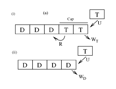
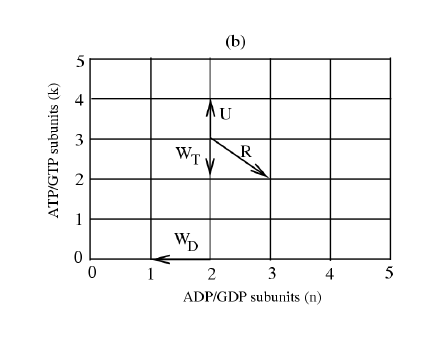
Figure 1: (a) Schematic diagram showing addition with rate $U$, removal with rates $W_{T}$ and $W_{D}$, and hydrolysis with rate $R$: (i) for the case where the cap length is non-zero and (ii) for the case where the cap length is zero. T stands for ATP (GTP) bound actin (microtubule) subunits while D stands for hydrolyzed ADP(GDP) subunits. At the T-D interface shown in (i), the hydrolysis occurs with a rate $R$. (b) Equivalent representation of the model as a biased random walk in the upper quarter 2D plane with rates $U$ to go up(north), $W_{T}$ to go down (south), $R$ to go south-east and $W_{D}$ to go west. The $W_{D}$ move is only possible along the $k=0$ (southern boundary) line.

The actin filament dynamics is studied in terms of two variables $n$, the number of ADP subunits, and $k$, the number of ATP subunits, as shown in figure 1. The dynamics of this system may be represented as a biased random walk in the upper quarter 2D plane $(n,k)$. For instance, the addition of one ATP subunit with rate $U$ corresponds to a move in the upward direction. The removal of ATP subunits with $W_{T}$ corresponds to a move in the downward direction. The hydrolysis of an ATP subunit results in an increase in $n$ and decrease in $k$, both by one unit, which corresponds to a move in the diagonal direction as shown in the figure. The removal of ADP subunits can happen only when the cap is zero and therefore corresponds to a leftward move along the $k=0$ line. Let $P(n,k,t)$ be the probability of having $n$ hydrolyzed ADP subunits and $k$ unhydrolyzed ATP subunits at time $t$, such that $l=(n+k)d$ is the total length of the filament. It obeys the following master equation: For $k>0$ and $n\geq 0$ we have

$$\frac{dP(n,k,t)}{dt}=UP(n,k-1,t)+W_{T}P(n,k+1,t)+RP(n-1,k+1,t)-(U+W_{T}+R)P(n,k,t).$$ (1)

When $n=0$ in Eq. 1, $P(-1,k+1,t)$ is set equal to zero.

For $k=0$ and $n\geq 1$ we have,

$$\frac{dP(n,0,t)}{dt}=W_{D}P(n+1,0,t)+W_{T}P(n,1,t)+RP(n-1,1,t)-(U+W_{D})P(n,0,t).$$ (2)

If $k=0$ and $n=0$, we have

$$\frac{dP(0,0,t)}{dt}=W_{T}P(0,1,t)+W_{D}P(1,0,t)-UP(0,0,t).$$ (3)

The sum of the probabilities is normalized to $1$ such that

$$\sum_{n=0}^{\infty}\sum_{k=0}^{\infty}P(n,k,t)=1.$$ (4)

We define the following generating functions

$$F_{k}(x,t) = \sum_{n\geq 0}P(n,k,t)x^{n},$$ (5)

$$H_{n}(y,t) = \sum_{k\geq 0}P(n,k,t)y^{k},$$ (6)

$$G(x,y,t) = \sum_{n\geq 0}\sum_{k\geq 0}P(n,k,t)x^{n}y^{k}$$ (7)

All quantities of interest can be computed from $G(x,y,t)$. For instance, the average length of the filament is

$$\langle l\rangle=\left[\langle n\rangle+\langle k\rangle\right]d=d\left(\frac{\partial G(x,1,t)}{\partial x}\right)_{x=1}+d\left(\frac{\partial G(1,y,t)}{\partial y}\right)_{y=1},$$ (8)

where $\langle k\rangle$ is the average number of the ATP subunits and $\langle n\rangle$ is the average number of the ADP subunits. The average velocity of the filament is

$$v=\lim_{t\to\infty}\frac{d\langle l\rangle}{dt},$$ (9)

and the diffusion coefficient is

$$D=\lim_{t\to\infty}\frac{1}{2}\frac{d}{dt}\left(\langle l^{2}\rangle-\langle l\rangle^{2}\right).$$ (10)

Similarly, the average velocity of the cap is

$$J=\left[\lim_{t\to\infty}\frac{d\langle k\rangle}{dt}\right]d,$$ (11)

and the diffusion coefficient of the cap is

$$D_{c}=\lim_{t\to\infty}\frac{d^{2}}{2}\frac{d}{dt}\left(\langle k^{2}\rangle-\langle k\rangle^{2}\right).$$ (12)

The solution of Eqs. 1, 2, and 3 and the details of the calculations are given in the Appendix A.

Phase diagram

Our model for the dynamics of a single filament with ATP hydrolysis leads to the following steady-state phases: a bound phase (phase I), an intermediate phase (phase II) and a rapidly growing phase (phase III). In phase I, the bound phase, the average velocity of the filament $v_{I}$ and the average velocity of the cap both vanish. Thus, the average filament and cap lengths remain constant in the long time limit. In phase $II$, the filament is growing linearly in time, with a velocity $v_{II}$, but the average ATP cap length remains constant as a function of time. In phase $III$, the filament as well the ATP cap are growing linearly in time with a filament velocity $v_{III}$ and cap velocity $J$. The boundary between phases I and II is the curve of equation $v_{II}=0$, and the boundary between phase II and III is the curve of equation $J=0$.

We have carried out simulations of the dynamics of the length of the filament, using the Gillespie algorithm (25). According to this algorithm, the time to the next on-, off-, or hydrolysis-event is computed stochastically at each step of the simulation. We find that our simulation results agree with the exact calculations.

The Bound phase (Phase I)

In the representation of the model as a biased random walk shown in figure 1, there is a regime of parameters for which the biased random walker converges towards the origin. After some transient time, the random walker enters what we call a bound steady state, where the motion of the walker is confined to a bounded region containing the origin. In the representation of the model as a filament, the filament length fluctuates as function of time around a time-independent average value $\langle l\rangle$ and at the same time, the cap length also fluctuates as function of time around a different time-independent average value $\langle k\rangle d$. A typical evolution of the total length of the filament $l(t)$, obtained from our Monte Carlo simulations, is shown in Fig. 2.

Figure 2: Filament length as a function of time for the three different phases of the model, as computed using Monte Carlo simulations. The value of the rates which were used are given in Table 1. Figure (a) represents the bound phase (phase I), where a structure of avalanches in the evolution of the length can be seen. These avalanches correspond to series of sudden depolymerization events (collapse) followed by slow polymerization events (rescue). Figure (b) represents the intermediate phase (phase II) and the rapidly growing phase (phase III). In the intermediate phase (II), the dynamics show large length fluctuations as compared to the rapidly growing phase (III), where the length fluctuations can hardly be resolved.

	$k_{0}$ ($\mu$m${}^{-1}s^{-1}$)	$W_{T}$($s^{-1}$)	$W_{D}$($s^{-1}$)	$R$ ($s^{-1}$)	d (nm)
Actin	11.6	1.4	7.2	0.3	2.7
Microtubule	3.2	24	290	4	0.6

Table 1: Numerical estimates of the rates $W_{T}$, $W_{D}$, $R$, $k_{0}$ and subunit length $d$. The parameters for actin are taken from refs. (2, 24) and they characterize the barbed end of an actin filament. The parameters for microtubule hold similarly for the plus end and at $35^{\circ}$C. The rate constant $k_{0}$ and rate $W_{D}$ are taken from (2), while the other two rates, $W_{T}$ and $R$, are deduced from fitting the zero-force velocity data of ref. (26) and the critical concentration measurements of ref. (27).

We first discuss the properties of the cap before considering that of the total length. In the steady state ($t\rightarrow\infty$), $F_{k}(x=1)$ represents the distribution of cap lengths, as defined in Eq. 5. As shown in the Appendix A,

$$F_{k}(x=1)=(1-q)q^{k},$$ (13)

where

$$q=\frac{U}{W_{T}+R}.$$ (14)

Since $F_{0}=1-q$, we see that $q$ has the meaning of the probability of finding a non-zero cap in the steady state (24). We consider for the moment only the case $q\leq 1$, which corresponds to phases I and II. From $F_{k}(x=1)$, we find that the average number of cap subunits is given by

$$\langle k\rangle=\frac{q}{1-q},$$ (15)

and

$$\langle k^{2}\rangle=\frac{q+q^{2}}{(1-q)^{2}}.$$ (16)

As expected, these quantities diverge when approaching the transition to phase III when $q\rightarrow 1$. The standard deviation of the cap length is

$$\sigma_{c}^{2}=\langle k^{2}\rangle-\langle k\rangle^{2}=\frac{q}{(1-q)^{2}}.$$ (17)

The relative fluctuations in the cap size are large since

$$\frac{\sigma_{c}^{2}}{\langle k\rangle^{2}}=\frac{1}{q}>1.$$ (18)

We now investigate the overall length of the filament in the bound phase. This quantity together with the distribution of length in the bound phase can be obtained from the time-independent generating function $G(x,y)$. The details of the calculation of this quantity are given in appendix A. We find

$$G(x,y)=\frac{\left(W_{T}+Rx\right)\left(\frac{W_{D}}{U}-\frac{W_{D}+R}{W_{T}+R}\right)\left(x-1\right)}{(y-y_{+})[W_{T}(y_{-}-1)x+Rx(y_{-}-x)+W_{D}y_{-}(1-x)]},$$ (19)

where $y_{\pm}$ are defined by

$$y_{\pm}=\frac{1}{2U}\left(U+W_{T}+R\pm\sqrt{(U+W_{T}+R)^{2}-4U(W_{T}+Rx)}\right).$$ (20)

From the derivatives of $G(x,y)$, we obtain analytically the average length $\langle l\rangle$ using Eq. 8 as

$$\langle l\rangle = \left[\frac{q\left(R^{3}+W_{D}R^{2}+2R^{2}W_{T}+W_{T}^{2}R+2W_{D}W_{T}R+W_{D}W_{T}^{2}\right)}{v_{II}(q-1)(W_{T}+R)^{2}}\right]d^{2}$$ (21)

$$-\left[\frac{q^{2}\left(R^{2}+2W_{T}R+W_{D}W_{T}\right)}{v_{II}(q-1)(W_{T}+R)}\right]d^{2},$$

where $v_{II}$ is the shrinking velocity (since $v_{II}<0$ in this regime) of the filament

$$v_{II}=\left[\frac{U(W_{D}+R)}{W_{T}+R}-W_{D}\right]d.$$ (22)

The length $\langle l\rangle$ diverges since $v_{II}\rightarrow 0$ when approaching the transition line between phases I and phase II. The length $\langle l\rangle$ as given by Eq. 21 is plotted in Fig. 3 for the parameters of table I. We compare this exact expression with the result of our Monte Carlo simulations where the average is computed using 1000 length values taken from different realizations. Excellent agreement is found with the analytical expression of Eq. 21. According to a simple dimensional argument, the average length $\langle l\rangle$ should scale as $-D_{II}/v_{II}$, where $D_{II}$ and $v_{II}$ are the diffusion coefficient and velocity of phase II. We find that this scaling argument actually holds only close to the transition point between phase I and II. On the boundary line between phases I and II, the average filament velocity vanishes and hence the filament length is effectively undergoing an unbiased “random walk”. In such a case, we expect that on the boundary line $\langle l^{2}\rangle\sim t$. We have also considered the fluctuations of $l(t)$ using the standard deviation $\sigma$ defined as

$$\sigma^{2}=\langle l^{2}\rangle-\langle l\rangle^{2},$$ (23)

for which an explicit expression can be obtained from $G(x,y)$. In Fig. 3, $\sigma$ is shown as a function of $U$. Note that $\sigma$ is larger than $\langle l\rangle$, which corresponds to dynamic-instability-like large length fluctuations.

In the limit $R\rightarrow 0$, ATP hydrolysis can be ignored in the assembly process. The model is then equivalent to a simple 1D random walk with rates of growth $U$ and decay $W_{T}$. In this case, phases II and III merge into a single growing phase. We find from Eq. 21 that $\langle l\rangle=Ud/(W_{T}-U)$, which diverges as expected near the transition to the growing phase when $U\simeq W_{T}$. According to the simple dimensional argument mentioned above, this length must scale as $-D/v$ in terms of the diffusion coefficient and velocity of the growing phase (14). This is the case, since $D=d^{2}(U+W_{T})/2$ and $v=(U-W_{T})d<0$ and thus $\langle l\rangle=Ud/(W_{T}-U)$ near the transition point.

Figure 3: Average length $\langle l\rangle$ and its standard deviation $\sigma$ in the bound phase for (a) actin, and (b) microtubule as a function of the insertion rate, $U$(lower x-axis), and of the concentration of the free ATP/GTP subunits $C$ (upper x-axis). The solid lines represent analytical expressions of $\langle l\rangle$ (lower curves) and $\sigma$ (upper curves). Filled symbols represent values obtained from simulations for these quantities. All the curves and symbols are obtained using values of the rates given in Table. 1.

We have also computed the filament length distribution, $P(l)$ in this phase using Monte Carlo simulations, as shown in Fig. 4.

Figure 4: Filament length distribution in the bound phase for actin. (a) For U=1.5 $s^{-1}$ and (b) for U=1.6 $s^{-1}$ with all other parameters taken from Table 1. The inset shows the same quantities ($l$ vs P(l)) with $P(l)$ in the log scale. The straight line in the inset is given by Eq. 24.

In the inset, we compare the numerically obtained distribution with the following exponential distribution

$$P(l)=P_{0}\exp{(-l/\langle l\rangle)},$$ (24)

where $\langle l\rangle$ is given by Eq. 21. In this figure, the distribution appears to be close to this exponential distribution. For any exponential distribution, the standard deviation, $\sigma$ should equal the mean $\langle l\rangle$. However as seen in figure 3, there is a difference between $\sigma$ and $\langle l\rangle$. Hence the distribution can not be a simple exponential, which could also have been guessed from the fact that the expression of $G(x,y)$ is complicated. The exact analytical expression of the distribution could be calculated by performing an inverse Z-transform of the known $G(x,y)$.

In the bound phase, experiments with actin in ref. (19) report an average length in the 5-20 $\mu$m range at different monomer concentrations, and experiments with microtubules of ref. (27) report a range 1-20 $\mu$m at different temperatures. Neither experiment corresponds precisely to the conditions for which the rates of table 1 are known. Thus a precise comparison is not possible at the moment, although we can certainly obtain with the present approach an average length in the range of microns using the rates of table 1 as shown in figure 3.

Intermediate phase (Phase II)

In the intermediate phase (phase II), the average ATP cap length remains constant as a function of time, while the filament grows linearly with time. The presence of this cap leads to interesting dynamics for the filament. A typical time evolution of the filament length is shown in figure 2. One can see the filament switching between growth (polymerization) and decay (depolymerization) in a way which is completely analogous to what is observed in the microtubule dynamics (12).

In this phase II, the average velocity of the filament is

$$v_{II}=\left[U-W_{T}q-W_{D}(1-q)\right]d.$$ (25)

This expression of $v_{II}$ is the same as Eq. 22 except that now Eq. 25 corresponds to the regime where $v_{II}>0$. The diffusion coefficient in this phase is

$$D_{II}=\frac{d^{2}}{2}\left[U+W_{T}q+W_{D}(1-q)+\frac{2(W_{D}-W_{T})(U+W_{D}q)}{W_{T}+R}\right].$$ (26)

The expressions of $v_{II}$ and $D_{II}$ are derived in the appendix A. When $d$ equals to half the size of an actin subunit, we recover exactly the expressions of ref. (24).

The transition between the bound phase (I) and the intermediate phase (II) is delimited by the $v_{II}=0$ curve. When going from phase $I$ to $II$, the average length in Eq. 21 varies as $\left(U-W_{D}\left(\frac{W_{T}+R}{W_{D}+R}\right)\right)^{-1}$, and the variance of the length $\sigma^{2}$ varies as $\left(U-W_{D}\left(\frac{W_{T}+R}{W_{D}+R}\right)\right)^{-2}$. The transition from the intermediate phase II to the rapidly growing phase III is marked by a similar behavior. The cap length diverges as $(U-W_{T}-R)^{-1}$, and the variance of the fluctuations of the cap length diverges as $(U-W_{T}-R)^{-2}$.

Rapidly Growing Phase (Phase III)

In phase III, the length of the ATP cap and that of the filament are growing linearly with time. Thus the probability of finding a cap of zero length is zero in the limit $t\rightarrow\infty$, that is $F_{0}(x=1)=0$. This also means that the probability of having a filament of zero length is also zero, i.e. P(0,0)=0. In this case, Eq. 49 reduces to

$$\frac{dG(x,y,t)}{dt}=\left[U\left(x-1\right)+W_{T}\left(\frac{1}{y}-1\right)+R\left(\frac{x}{y}-1\right)\right]G(x,y,t).$$ (27)

Using Eqs. 53, 54, 55 and 56 of Appendix A, one can easily obtain the following quantities

$$v_{III} = \left[U-W_{T}\right]d,$$ (28)

$$D_{III} = \frac{d^{2}}{2}\left(U+W_{T}\right),$$ (29)

$$J = \left[U-(W_{T}+R)\right]d,$$ (30)

$$D_{c} = \frac{d^{2}}{2}\left(U+W_{T}+R\right).$$ (31)

Note that these quantities can be obtained from Eqs. 25-26 by taking the limit $q\rightarrow 1$, which marks the transition between phase III and phase II. In Fig. 2, the filament length is plotted as a function of time. Note that in this phase the velocity and the diffusion coefficient are the same as those of a filament with no ATP hydrolysis. The physical reason is that in phase III, the length of the non-hydrolyzed region (cap) is very large and the region with hydrolyzed subunits is never exposed.

Effect of force and actin concentration on active polymerization

The driving force of self-assembly of the filament is the difference of chemical potential between bound and unbound ATP actin subunits. Since the chemical potential of unbound ATP actin subunits depend on the concentration $C$ of free ATP actin subunits and on the external applied force $f$, the rates should depend also on these physical parameters. In the biological context, this external force corresponds to the common situation where a filament is pushing against a cell membrane. For the concentration dependance, we assume a simple first order kinetics for the binding of ATP actin monomers given that the solution is dilute in these monomers. This means that the rate $U$ of binding of ATP actin is proportional to $C$ while $W_{T}$, $W_{D}$, and $R$ should be independent of $C$ (28, 29, 30). For the force dependance of the rates, general thermodynamical arguments only enforce a constraint on the ratio of the rates of binding to that of unbinding (31, 2). A simple choice consistent with this and supported by microtubule experiments (32) is to assume that only the binding rate i.e. $U$ is force dependent. A more sophisticated modeling of the force dependance of the rates has been considered for instance for microtubules in (33). All the constraints are then satisfied by assuming that $U=k_{0}C\exp{(-fd/k_{B}T)}$, with $k_{0}$, $W_{T}$, $W_{D}$, and $R$ all independent of the force $f$ and of the concentration $C$. We assume that $f>0$, so that the on-rate is reduced by the application of the force. The cap velocity in the rapidly growing phase(phase III), given by Eq. 30, can be written in terms of $f$ and $C$ as

$$J(f,C)=\left[k_{0}Ce^{-fd/k_{B}T}-(W_{T}+R)\right]d.$$ (32)

The phase boundary between phase II and phase III is defined by the curve $J(C,f=f_{c})=0$. Equating the cap velocity to zero, we obtain the characteristic force,

$$f_{c}=-\frac{k_{B}T}{d}\ln{\left[\frac{W_{T}+R}{k_{0}C}\right]}=-\frac{k_{B}T}{d}\ln{\frac{C_{0}}{C}}.$$ (33)

where the concentration $C_{0}$ is defined as

$$C_{0}=(W_{T}+R)/k_{0}.$$ (34)

Below $f_{c}$, the system is in phase III. This is also the point where $q=1$.

The force-velocity relation in the intermediate phase is rewritten, using Eq. 25, as

$$v_{II}(f,C)=k_{0}Ce^{-fd/k_{B}T}\left[\frac{W_{D}+R}{W_{T}+R}\right]d-W_{D}d.$$ (35)

The stall force $f_{s}$ is by definition the force at which $v_{II}(f=f_{s},C)=0$. From Eq. 35, we obtain

$$f_{s}=-\frac{k_{B}T}{d}\ln{\left[\left(\frac{W_{T}+R}{W_{D}+R}\right)\frac{W_{D}}{k_{0}C}\right]},$$ (36)

which can be written equivalently in terms of the critical concentration of the barbed end $C_{crit}$ as

$$f_{s}=-\frac{k_{B}T}{d}\ln{\left(\frac{C_{crit}}{C}\right)},$$ (37)

where

$$C_{crit}=C_{0}\left(\frac{W_{D}}{W_{D}+R}\right)<C_{0}.$$ (38)

In the absence of hydrolysis, when $R\rightarrow 0$, we have $C_{crit}=C_{0}$ and Eq. 37 gives the usual expression of the stall force given in the literature (2, 34, 28, 29)

The velocity of the filament is shown in Fig. 5 with a zoomed in version marked as (b).

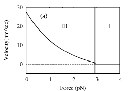
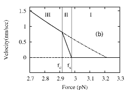
Figure 5: (a) Steady-state force-velocity relation for a single actin filament shown for $C=1\mu$M (solid curve), (b) Zoom of the force-velocity relation near the stall force. The vertical lines represent $f_{c}$ and $f_{s}$ as shown in figure (b). For $f<f_{c}$, the filament is in the rapidly growing phase (III) and the velocity is given by Eq. 28. In the bound phase (I) the velocity is zero. In the intermediate phase the velocity is given by Eq. 25. The dash-dotted line (figure (b), phase I and II) is given by Eq. 28, showing that the stall force is higher when ATP hydrolysis is neglected.

This figure shows that for $f<f_{c}$, the filament is in phase III, and that there the velocities of the filament with ATP hydrolysis or without are the same. At $f=f_{c}$, the force-velocity curve changes its slope, as shown after the vertical line in figure 5 (see the zoomed-in figure 5b). When the concentration rather than the force is varied, a similar change of slope is observed at $C=C_{0}$, which is accompanied by a discontinuity of the diffusion coefficient slightly above the critical concentration (24).

For $f_{c}<f<f_{s}$, the filament is in the intermediate phase, where the velocities in the presence and in the absence of ATP hydrolysis differ. The stall force with ATP hydrolysis is smaller than that in the absence of ATP hydrolysis. In view of this, a useful conclusion is that it is important to take into account the ATP hydrolysis for estimating the velocity of a filament when the force is close to the stall force.

For $f>f_{s}$, the velocity of the filament vanishes. It must be noted that, in this phase, the instantaneous velocity can be positive or negative, but the average velocity, in the long time limit, is zero. Another important point to note is that when the filament is stalled, ATP is still hydrolyzed. This is analogous with models of molecular motors containing more than one cycle (35, 36, 37). Including the chemical cycle of ATP hydrolysis in addition to the mechanical cycle of addition/removal of subunits is for this reason important in the context of actin and microtubule models. One could imagine testing these predictions on the effect of ATP hydrolysis on force-velocity relations by carrying out force-velocity measurements near stalling conditions of abundant ATP or when ATP is sequestered by appropriate proteins (38).

All these observations can be summarized in a phase diagram in the coordinates $f$ and $C$ as shown in Fig. 6.

Figure 6: Phase diagram as a function of the normalized force $fd/k_{B}T$ and of the log of the ratio of the ATP subunit concentration $C$ to the characteristic concentration $C_{0}$ for actin. The phase diagram shows the bound phase (phase I), the intermediate phase (phase II), and the rapidly growing phase (phase III). The boundary line between phase II and phase III is the curve $J=0$ and the boundary line between phase I and phase II is the curve $v_{II}=0$.

As shown in Fig. 6, when $C<C_{0}$, the filament is either in the intermediate phase (II) or in the bound phase (I). In this region of the phase diagram, the fluctuations of the filament length are large as compared to the very small fluctuations observed in the rapidly growing phase (III). The large fluctuations observed in phase I correspond to the dynamic instability.

In the case of microtubules, we find as shown in Table 2, $C_{0}=8.75\mu{\rm M}$. This value is rather large when compared to typical experimental concentrations $C\simeq 1-10\mu{\rm M}$ for microtubules. Thus microtubules are usually found in phases I and II where the length fluctuations are large and dynamic instability is commonly observed.

In the case of actin, we find that $C_{0}=0.147~{}\mu{\rm M}$. Typical experimental actin concentrations are above this estimate, therefore, at zero force, actin filaments are usually seen in phase III. This may explain why the dynamic instability is rarely seen in actin experiments with pure actin. However, at small concentrations close to the critical concentration, large length fluctuations have been observed for actin (19).

	$C_{0}\,(\mu$M)	$C_{crit}\,(\mu$M)	$f_{c}$ (pN)	$f_{s}$ (pN)
Actin	0.147	0.141	2.916 (at 1 $\mu$M)	2.978 (at 1 $\mu$M)
Microtubule	8.75	8.63	5.65 (at 20 $\mu$M)	5.74 (at 20 $\mu$M)

Table 2: Estimates of the characteristic concentrations $C_{0}$ and $C_{crit}$ at zero force, and of the characteristic forces $f_{c}$ and $f_{s}$ at a concentration of 1 $\mu$M for actin and 20 $\mu$M for microtubule using the rates of Table 1.

When discussing the effect of force on a single actin or microtubule filament, one important issue is the buckling of the filament. Since actin filaments have much smaller persistence length $l_{p}$ than microtubules, actin filaments buckle easily under external force. Our approach is appropriate to describe experiments like that of ref (34), where very short actin filaments are used. The length of the filaments must be smaller than the critical length for buckling under a force $f$. This length can be estimated as $l_{b}=\pi\sqrt{\kappa/f}$ with a hinged boundary condition, where $\kappa=l_{p}k_{B}T$. Taking $l_{p}\approx 17\mu$m, we estimate $l_{b}\approx 828$nm at $f=1$pN. Our discussion of the force will be applicable only for filaments shorter than $l_{b}$.

Collapse time

In this new section, we shall study experimentally relevant questions such as the mean time required for the ATP cap to disappear or the mean time required for the whole filament (ATP cap and ADP subunits) to collapse to zero length. We are interested in the conditions for which these times are finite. Below we address these questions.

Cap collapse in phases I or II

The dynamics of the cap corresponds to that of a 1D biased random walker with a growth rate $U$ and a decay rate $W_{T}+R$. Here, we calculate the mean time $T_{k}$ required for a cap of initial length $k$d to reach zero length for the first time. We assume that there is a bias towards the origin so that $W_{T}+R>U$. This time $T_{k}$ is nothing but the mean first passage time for the biased random walker to reach $k=0$, starting from an arbitrary site $k$ in phases I or II. According to the literature on first passage times, the equation for $T_{k}$ is (39, 40, 41) :

$$UT_{k+1}+(W_{T}+R)T_{k-1}-(U+W_{T}+R)T_{k}+1=0.$$ (39)

When $W_{T}+R>U$, this recursion relation can be solved (see Appendix B) with the condition that $T_{0}=0$, and we obtain

$$T_{k}=\frac{k}{W_{T}+R-U}.$$ (40)

This corresponds to the time the random walker takes to travel a distance $k$ at a constant velocity $-J$. Note that the mean first passage time $T_{k}$ becomes infinite in the unbiased case when $J=0$ or if the bias is not towards the origin i.e. when $W_{T}+R\leq U$ (which would correspond to an initial condition in phase III) (39).

One can also define an average of the mean first passage time with respect to the initial conditions. Averaging over $k$ and using equation (15), one obtains

$$\langle T_{k}\rangle=\frac{U}{(W_{T}+R-U)^{2}}.$$ (41)

The same time can be recovered by considering the average time associated with the fluctuation of the cap:

$$\langle T_{k}\rangle=\frac{\langle k^{2}\rangle d^{2}}{2D_{c}}.$$ (42)

This time may be related to the catastrophe rate in the following way. In ref. (14), the catastrophe rate is defined as the total number of catastrophes observed in an experiment divided by the total time spent in the growing phase. Since the growing phase ends when the cap disappears for the first time, we interpret similarly $1/\langle T_{k}\rangle$, as an average collapse frequency of the cap.

Filament collapse in phase I

Now we consider the dynamics of the filament length which is described similarly by a 2D biased random walk converging towards the origin. Here we investigate the mean time $T_{n,k}$ required for a filament with an initial state of $n$ ADP subunits and $k$ ATP subunits to reach zero length for the first time with an initial condition inside phase I. Again, this is the mean first passage time now in a 2D domain (in the $n-k$ plane, as shown in Fig. 1) to reach the origin ($n=0,k=0$) starting from an arbitrary $n$ and $k$. This mean first passage time $T_{n,k}$ obeys the following set of equations (39). When $k>0$, for all $n$, the equation is

$$UT_{n,k+1}+W_{T}T_{n,k-1}+RT_{n+1,k-1}-(U+W_{T}+R)T_{n,k}+1=0.$$ (43)

For $k=0$ and $n>0$ we have a special equation

$$UT_{n,1}+W_{D}T_{n-1,0}-(U+W_{D})T_{n,0}+1=0,$$ (44)

and we also have the condition $T_{00}=0$.

The simplest way to solve these equations is to guess by analogy with the 1D case that the solution must be a linear function of $n$ and $k$. This leads to a simple ansatz of the form $T_{n,k}=An+Bk$, which in fact gives the exact result as can be shown rigorously. Substituting this in Eq. 43 and Eq. 44, we can solve for unknowns $A$ and $B$. This leads to

$$T_{n,k}=\frac{nd}{-v_{II}}+\frac{kd}{-v_{II}}\left(\frac{W_{D}+R}{W_{T}+R}\right)$$ (45)

where $v_{II}$ is the velocity of the intermediate phase given by Eq. 25. Note that $v_{II}<0$ here since the initial condition is within phase I.

We first examine some simple particular cases of Eq. 45. As we approach the intermediate phase boundary $v_{II}\rightarrow 0$, $T_{n,k}\rightarrow\infty$ as expected. When $W_{D}=\infty$, $T_{n,k}=k/(W_{T}+R-U)=T_{k}$, which is the cap collapse time calculated in the 1D case. When $W_{D}=\infty$, the whole filament collapses immediately after the cap has disappeared for the first time i.e. after a time $T_{k}$. When $R\rightarrow\infty$, ATP subunits instantaneously become ADP subunits and we obtain another simple result $T_{n,k}={(n+k)/(W_{D}-U)}$. We have also compared the prediction of Eq. 45 with Monte Carlo simulations in Fig. 7 and we have found an excellent agreement.

Figure 7: Mean time taken by a filament of initial length $(n+k)d$ to collapse to zero length. Curves are given by eq. 45 and points are obtained from a Monte Carlo simulation for different values of $n$ and $k$. From bottom to top $(n,k)=(990,10),(750,250),(500,500)$ and $(200,800)$.

We can also define an average of the above mean first passage time where the average is performed over initial lengths of cap and un-hydrolyzed region. Averaging over $k$ and $n$ in Eq. 45 we obtain

$$\langle T_{n,k}\rangle=\frac{U(R^{2}+W_{D}R+W_{T}R+W_{D}^{2})}{\left(UR-W_{D}W_{T}-W_{D}R+UW_{D}\right)^{2}}.$$ (46)

The inverse, $1/\langle T_{n,k}\rangle$, can be called the collapse frequency of the filament. The filament collapse frequency and the cap collapse frequency are shown in Fig. 8 as a function of $U$ and $C$ for the cases of actin and microtubule using parameters of Table 1. Both frequencies are close to each other because the rate $W_{D}$ is large compared to other rates (see Table 1). This figure also shows that as the frequency of collapse is increased, the rate $U$ decreases and so the filament length is decreasing, which is expected (14). The behavior of the collapse frequency as function of the growing velocity in the absence of force agrees with (26). The decrease of the rate of monomer addition is in practice caused by either the application of a force or a lowering of the concentration. Thus the application of force may be seen as a general mechanism to regulate the dynamic instability.

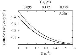
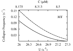
Figure 8: Collapse frequencies for actin and microtubule(MT) as function of the rate of addition of monomers $U$ (lower x-axis) and of the concentration $C$ (upper x-axis): Solid line represents the collapse frequency of the filament given by, $1/\langle T_{n,k}\rangle$, the inverse of the time given in Eq. 46. Dashed line represents the collapse frequency of the cap given by, $1/\langle T_{k}\rangle$, the inverse of the time given in Eq. 41.

In the opposite limit, when $R/W_{D}\rightarrow 0$ one can also understand the result physically from the following argument. When the filament collapses, the first event is the disappearance of the cap and therefore the first contribution to the collapse time is the mean time required for the cap to disappear, $T_{k}$, as obtained from Eq. (40). Once the cap has disappeared, assuming that $W_{D}$ is very large, ADP subunits start depolymerizing until the next ATP subunit addition takes place. The mean time needed for an ATP subunit addition to take place is $1/U$. Once an ATP subunit is added, one has to wait an average time of $T_{1}$ for the cap to disappear again. This cycle of ATP subunit addition and depolymerization repeats many times. The number of times this cycle occurs, starting with a filament of $n$ ADP subunits, is roughly $n/(\frac{W_{D}}{U})$. But one also has to take into account the increase in ADP subunits as a result of ATP hydrolysis, which is done by subtracting $RT_{1}$ from $n/(\frac{W_{D}}{U})$. This leads to the following approximate expression for $T_{n,k}$

$$T_{n,k} \simeq T_{k}+\left[\frac{1}{U}+T_{1}\right]\frac{n}{(\frac{W_{D}}{U}-RT_{1})}.$$ (47)

$$\simeq \frac{nd}{-v_{II}}+\frac{kd}{-J}$$ (48)

where $J=(U-W_{T}+R)d$ is the cap velocity in the rapidly growing phase. This solves Eq. 43 and Eq. 44 in the limit $R/W_{D}\rightarrow 0$ and agrees reasonably well with the Monte Carlo simulations.

Conclusions

In this paper, we have studied a model for the dynamics of growth and shrinkage of single actin/microtubule filaments, taking into account the ATP/GTP hydrolysis which occurs in the polymerized filament. We find three dynamical phases with different properties of the ATP/GTP cap and the filament: a bound phase, an intermediate phase and a rapidly growing phase. For each phase, we have calculated the steady-state properties of the non-hydrolyzed cap and of the filament and we have investigated the role of an external force (f) applied on the filament during polymerization and of the monomer concentration (C), leading to a f-C phase diagram. We have also calculated the collapse time which is the time needed for the cap or the filament to completely depolymerize.

In the bound phase, both the size of the filament and the size of the cap are finite. It must be noted that in batch experiments, where the total (free+bound) concentration of monomers is a constant, the steady state is always the bound phase. If the total monomer concentration is large enough, the filament length is very large and the concentration in the bound phase will be just below the critical concentration. The filaments exhibit large length fluctuations in the bound phase corresponding to the dynamic instability observed with microtubules. An important conclusion is the role of ATP/GTP hydrolysis in determining the stall force of the filament: the effect of hydrolysis always reduces the value of the stall force. Dynamic instabilities are in general not observed with actin filaments when no force is applied to the filament. However, in recent experiments  (21, 22), it has been found that the presence of ADF/Cofilin leads to a bound phase even at zero force where actin filaments exhibit large length fluctuations. In the absence of binding proteins, a natural way to regulate the dynamic instability and the length of the filament is through the application of force.

The intermediate phase is a phase where the filaments grow at a constant velocity with a finite ATP/GTP cap. This is the phase which is in general observed in a cell. There are large length fluctuations of the cap in this phase but the length fluctuations are not as large as the average length. Thus, there is no true dynamic instability in this phase but we give predictions for the typical time of the collapse of the cap. Finally, the growth phase corresponds to the case where both the filament and the cap grow at a constant velocity.

One of the limitations of our work is that we considered a single protofilament. This does not seem to be an important issue for actin filaments where the length difference between the two protofilaments is always small and of the order of an actin monomer. For microtubules, the detailed polymerization mechanism seems to be very complex and this certainly plays an important role on the way the force is distributed between protofilaments (42). Recent experiments have also considered the maximum force that can be generated by a bundle of parallel actin filaments (34). Our results raise interesting questions about the role of ATP hydrolysis in this case.

Our work could be extended in several directions. In the biological context, actin or microtubule polymerization is regulated by capping proteins and it would be important to understand quantitatively the regulation mechanism and to incorporate them in our model. This is for example the case for motors of the Kin-13 family that have been found to interact with microtubules and induce filament depolymerization (43). So far, we have mainly considered the polymerization kinetics, but in general, there is a complex interplay between the mechanical properties of the filaments and the polymerization kinetics, which we plan to explore in future work.

Appendix

A. Calculations using the generating function approach

Summing over $n$ and $k$ in Eq. 1 and using equations 2, 3 and 7, one obtains

$$\frac{dG(x,y,t)}{dt} = \left[U\left(x-1\right)+W_{T}\left(\frac{1}{y}-1\right)+R\left(\frac{x}{y}-1\right)\right]G(x,y,t)$$ (49)

$$- \left[W_{T}\left(\frac{1}{y}-1\right)+R\left(\frac{x}{y}-1\right)+W_{D}\left(1-\frac{1}{x}\right)\right]F_{0}(x,t)$$

$$+ W_{D}\left(1-\frac{1}{x}\right)P(0,0,t).$$

Similarly one can also write down equations for $F_{k}$ and $H_{n}$. This equation contains $F_{0}$, which is coupled to all the $F_{k}$. For $k>0$,

$$\frac{dF_{k}(x,t)}{dt}=UF_{k-1}(x,t)+\left(W_{T}+Rx\right)F_{k+1}(x,t)-\left(U+W_{T}+R\right)F_{k}(x,t),$$ (50)

and for $k=0$,

$$\frac{dF_{0}(x,t)}{dt}=\left(W_{D}\left(\frac{1}{x}-1\right)-U\right)F_{0}(x,t)+\left(W_{T}+Rx\right)F_{1}(x,t).$$ (51)

Solving this set of equations we shall derive a formula for $G(x,y,t)$. From $G(x,y,t)$, we calculate the following quantities:

The average length

$$\langle l\rangle=\left[\langle n\rangle+\langle k\rangle\right]d=d\left(\frac{\partial G(x,1,t)}{\partial x}\right)_{x=1}+d\left(\frac{\partial G(1,y,t)}{\partial y}\right)_{y=1},$$ (52)

the velocity of the filament

$$v=\lim_{t\to\infty}\frac{d\langle l\rangle}{dt}=d\lim_{t\to\infty}\frac{\partial}{\partial x}\left(\frac{dG(x,x,t)}{dt}\right)_{x=1},$$ (53)

and the diffusion coefficient of the filament length

$$D = \lim_{t\to\infty}\frac{1}{2}\frac{d}{dt}\left(\langle l^{2}\rangle-\langle l\rangle^{2}\right)$$ (54)

$$= d^{2}\lim_{t\to\infty}\left[\frac{1}{2}\frac{\partial^{2}}{\partial x^{2}}\left(\frac{dG(x,x,t)}{dt}\right)+\frac{1}{2}\frac{\partial}{\partial x}\left(\frac{dG(x,x,t)}{dt}\right)\right.$$

$$\left.-\left(\frac{\partial G(x,x,t)}{\partial x}\right)\frac{\partial}{\partial x}\left(\frac{dG(x,x,t)}{dt}\right)\right]_{x=1}.$$

The average velocity of the cap is

$$J=d\lim_{t\to\infty}\frac{d\langle k\rangle}{dt}=\lim_{t\to\infty}\frac{\partial}{\partial y}\left(\frac{dG(1,y,t)}{dt}\right)_{y=1},$$ (55)

and the diffusion coefficient of the cap is

$$D_{c} = d^{2}\lim_{t\to\infty}\frac{1}{2}\frac{d}{dt}\left(\langle k^{2}\rangle-\langle k\rangle^{2}\right)$$ (56)

$$= d^{2}\lim_{t\to\infty}\left[\frac{1}{2}\frac{\partial^{2}}{\partial y^{2}}\left(\frac{dG(1,y,t)}{dt}\right)+\frac{1}{2}\frac{\partial}{\partial y}\left(\frac{dG(1,y,t)}{dt}\right)\right.$$

$$\left.-\left(\frac{\partial G(1,y,t)}{\partial y}\right)\frac{\partial}{\partial y}\left(\frac{dG(1,y,t)}{dt}\right)\right]_{y=1}.$$

Calculation of $F(x=1,t\rightarrow\infty)$ in phases I and II

In the steady-state ($t\rightarrow\infty$), the cap distribution in phases I and II becomes time-independent and hence $(dF_{k}/dt)_{x=1}=0$. In this case Eqs. 50 and 51 can be written, for $k>0$, as

$$0=UF_{k-1}+\left(W_{T}+R\right)F_{k+1}-\left(U+W_{T}+R\right)F_{k},$$ (57)

and for $k=0$,

$$0=\left(W_{T}+R\right)F_{1}-UF_{0}.$$ (58)

where we denote for short, $F_{k}=F_{k}(x=1,t\rightarrow\infty)$. The solution of Eq. 57 is of the form $F_{k}=q^{k}F_{0}$. If we substitute this back into Eq. 57, we get a quadratic equation in $q$

$$(W_{T}+R)q^{2}-(U+W_{T}+R)q+U=0.$$ (59)

The two solutions are $q=U/(W_{T}+R)$ and $q=1$, but we can rule out $q=1$ using the normalization condition $\sum_{k=0}^{\infty}F_{k}=1$. In phases I and II, $W_{T}+R>U$ and therefore $q<1$. Using the normalization condition, we obtain

$$F_{k}=(1-q)q^{k},$$ (60)

which is Eq. 13.

Calculation of $G(x,y)$ in the bound phase (phase I) .

We now explain how to calculate $G(x,y)$ in the bound phase, using a technique of canceling apparent poles  (40, 41). Since we are interested in the steady-state properties of the bound phase, the time derivative of $G$ on the left hand side of Eq. 49 is zero, which leads to

$$G(x,y)=\frac{F_{0}(x)\left[Rx(y-x)+W_{T}x(y-1)-W_{D}y(x-1)\right]-W_{D}P(0,0)y(1-x)}{x\left[-Uy^{2}+(U+W_{T}+R)y-Rx-W_{T}\right]},$$ (61)

where $F_{k}(x)$ and $P(0,0)$ are unknowns. By definition

$$G(x,y)=\sum_{n\geq 0}\sum_{k\geq 0}P(n,k)x^{n}y^{k},$$

since the $P(n,k)$ are bounded numbers, $G(x,y)$ is an analytic function for $0\leq|x|\leq 1$ and $0\leq|y|\leq 1$. To guarantee the analyticity of the function $G(x,y)$, the zero of the denominator of Eq. 61,

$$y=y_{-}=\frac{1}{2U}\left(U+W_{T}+R-\sqrt{(U+W_{T}+R)^{2}-4U(W_{T}+Rx)}\right),$$

must also be a zero of the numerator. This implies that

$$F_{0}(x)=\frac{W_{D}P(0,0)y_{-}(1-x)}{Rx(y_{-}-x)+W_{T}x(y_{-}-1)-W_{D}y_{-}(x-1)}.$$ (62)

The normalization condition, namely G(x=1,y=1)=1, then fixes the value of $P(0,0)$ as

$$P(0,0)=1-\frac{U}{W_{D}}\left(\frac{W_{D}+R}{W_{T}+R}\right).$$ (63)

After substituting Eqs. 62 and 63 into Eq. 61, we obtain the expression of $G(x,y)$ given in Eq. 19.

Velocity and diffusion coefficient in the Intermediate phase (phase II)

We recall the definition of $F_{k}(x,t)$ given in Eq. 7:

$$F_{k}(x,t)=\sum_{n\geq 0}P(n,k,t)x^{n},$$ (64)

and we recall that $F_{k}$ with no argument is a short notation for $F_{k}(x=1,t\rightarrow\infty)$. From this, we introduce

$$a_{k}(t)=\left(\frac{\partial F_{k}(x,t)}{\partial x}\right)_{x=1},$$ (65)

so that $<n(t)>=\sum_{k\geq 0}P(n,k,t)n=\sum_{k\geq 0}a_{k}(t)$.

By taking a derivative with respect to $x$ in Eqs. 50 and 51, one obtains the equations of evolution of $a_{k}(t)$: for $k>0$

$$\frac{da_{k}(t)}{dt}=Ua_{k-1}(t)+(W_{T}+R)a_{k+1}(t)-(U+W_{T}+R)a_{k}(t)+RF_{k+1}(x=1,t)$$ (66)

and for $k=0$

$$\frac{da_{0}(t)}{dt}=-W_{D}F_{0}(x=1,t)-Ua_{0}(t)+(W_{T}+R)a_{1}(t)+RF_{1}(x=1,t).$$ (67)

As shown in (24), there is a solution of these recursion relations in the long time limit in the form of $a_{k}(t)=M_{k}t+B_{k}$, where $M_{k}$ and $B_{k}$ are time independent coefficients. After substituting this equation into Eqs. 66-67, and separating terms which are time-dependent from terms which are not time-dependent, one obtains separate recursion relations for $M_{k}$ and $B_{k}$. The recursion relation of $M_{k}$ is identical to that of $F_{k}$ obtained in Eq. 57-58. Using Eq. 60, the solution can be written as $M_{k}=v_{II}(1-q)q^{k}/d=v_{II}F_{k}/d$. The recursion relation of $B_{k}$ is for $k>0$,

$$M_{k}=UB_{k-1}+(W_{T}+R)B_{k+1}-(U+W_{T}+R)B_{k}+RF_{k+1},$$ (68)

and for $k=0$,

$$M_{0}=-W_{D}F_{0}-UB_{0}+(W_{T}+R)B_{1}+RF_{1}.$$ (69)

These recursion relations can also be solved with the result

$$B_{k}=B_{0}q^{k}+\left[\frac{W_{D}(1-q)}{W_{T}+R}\right]kq^{k}.$$ (70)

To characterize the intermediate phase, it is convenient to rewrite the evolution equation for the generating function $G(x,y,t)$ of Eq. 49 using the fact that $P(0,0,t\rightarrow\infty)=0$ in this phase, in the form of an evolution equation for $\tilde{G}(x,t)=G(x,x,t)$ as

$$\frac{d\tilde{G}(x,t)}{dt}=\alpha(x)\tilde{G}(x,t)+\beta(x,t),$$ (71)

where $\alpha(x)=U(x-1)+W_{T}(1/x-1)$ and $\beta(x,t)=(1-1/x)(W_{T}-W_{D})F_{0}(x,t)$. With this notation, the velocity defined in Eq. 53 is

$$v=d\lim_{t\to\infty}\frac{\partial}{\partial x}\left(\frac{d\tilde{G}(x,t)}{dt}\right)_{x=1}=d\left[\alpha^{\prime}(1)+\beta^{\prime}(1,t\rightarrow\infty)\right],$$ (72)

where the prime denotes derivatives with respect to $x$. Substituting the expressions of $\alpha(x)$ and $\beta(x,t)$ into this equation, it is straightforward to obtain the velocity $v=v_{II}$ characteristic of the intermediate phase which is Eq. 25. Similarly, using Eq. 54 and Eq. 71, the diffusion coefficient can be written as

$$D=\frac{d^{2}}{2}\lim_{t\to\infty}\left[\alpha^{\prime\prime}(1)+\beta^{\prime\prime}(1,t)+\alpha^{\prime}(1)+\beta^{\prime}(1,t)-2\tilde{G}^{\prime}(1,t)\beta^{\prime}(1,t)\right],$$ (73)

where

$$\tilde{G}^{\prime}(1,t) = \left(\frac{\partial\tilde{G}(x,t)}{\partial x}\right)_{x=1}=\langle n(t)\rangle+\langle k\rangle,$$ (74)

$$= vt+\frac{1}{1-q}\left[B_{0}+\frac{U+W_{D}q}{W_{T}+R}\right].$$

After substituting Eq. 74 into Eq. 73 and simplifying, the terms linear in time and the term containing the unknown parameter $B_{0}$ cancel out in the expression of the diffusion coefficient, and we finally obtain $D=D_{II}$ which is given in Eq. 54.

B. Cap collapse time $T_{k}$

In order to solve the recursion relation for $T_{k}$ of Eq. 39, we perform a $z$ transformation defined by

$$\tilde{T}(z)=\sum_{k\geq 0}T_{k}z^{-k}.$$ (75)

After using the initial condition $T_{0}=0$, we obtain

$$\tilde{T}(z)=\frac{(1+UT_{1}(1-z))z}{U(1-z)^{2}(q^{-1}-z)}$$ (76)

where $q^{-1}=(W_{T}+R)/U$. By definition, $\tilde{T}(z)$ is analytic for all values of $|z|>1$. Since we are interested in the case $W_{T}+R>U$, the numerator in Eq. 76 must vanish to ensure that $\tilde{T}(z)$ is analytic at $z=q^{-1}$. This condition determines the unknown $T_{1}=1/(W_{T}+R-U)$. Now $T_{k}$ can be obtained by an inverse Z transform as

$$T_{k}=\frac{1}{2\pi i}\oint\tilde{T}(z)z^{k-1}dz=\frac{1}{2\pi i}\oint\frac{z^{k}dz}{U(1-z)^{2}(q^{-1}-1)}=\frac{k}{W_{T}+R-U}.$$ (77)

References

- Desai and Mitchison (1997) Desai, A., and T. J. Mitchison, 1997. Microtubule polymerization dynamics. Annual Review of Cell and Developmental Biology 13:83–117.
- Howard (2001) Howard, J., 2001. Mechanics of Motor Proteins and the Cytoskeleton. Sinauer Associates, Inc., Massachusetts.
- Schneider et al. (2002) Schneider, M. E., I. A. Belyantseva, R. B. Azevedo, and B. Kachar, 2002. Rapid renewal of auditory hair bundles. Nature 418:837–838.
- Rosenbaum and Witman (2002) Rosenbaum, J. L., and G. B. Witman, 2002. Intraflagellar transport. Nature Reviews Molecular Cell Biology 3:813–825.
- Prost et al. (2007) Prost, J., C. Barbetta, and J.-F. Joanny, 2007. Dynamical Control of the Shape and Size of Stereocilia and Microvilli. Biophys. J. 93:1124–1133.
- Liu et al. (1999) Liu, D., M. Martic, G. Clarke, M. Dunlop, and H. Baker, 1999. An important role of actin polymerization in the human zona pellucida-induced acrosome reaction. Mol. Hum. Reprod. 5:941–949.
- Shin et al. (2004) Shin, J. H., L. Mahadevan, P. T. So, and P. Matsudaira, 2004. Bending Stiffness of a Crystalline Actin Bundle. J. Mol. Biol. 337:255–261.
- Breitbart et al. (2005) Breitbart, H., G. Cohen, and S. Rubinstein, 2005. Role of actin cytoskeleton in mammalian sperm capacitation and the acrosome reaction. Reproduction 129:263–268.
- Hunt and McIntosh (1998) Hunt, A. J., and J. R. McIntosh, 1998. The Dynamic Behavior of Individual Microtubules Associated with Chromosomes In Vitro. Mol. Biol. Cell 9:2857–2871.
- Pantaloni et al. (1985) Pantaloni, D., T. L. Hill, M. F. Carlier, and E. D. Korn, 1985. A model for actin polymerization and the kinetic effects of ATP hydrolysis. Proc. Natl. Acad. Sci. USA. 82:7207–7211.
- Hill (1986) Hill, T. L., 1986. Theoretical study of a model for the ATP cap at the end of an actin filament. Biophys. J. 49:981–986.
- Dogterom and Leibler (1993) Dogterom, M., and S. Leibler, 1993. Physical aspects of the growth and regulation of microtubule structures. Phys. Rev. Lett. 70:1347–1350.
- Flyvbjerg et al. (1994) Flyvbjerg, H., T. E. Holy, and S. Leibler, 1994. Stochastic Dynamics of Microtubules: A Model for Caps and Catastrophes. Phys. Rev. Lett. 73:2372–2375.
- Flyvbjerg et al. (1996) Flyvbjerg, H., T. E. Holy, and S. Leibler, 1996. Microtubule dynamics: Caps, catastrophes, and coupled hydrolysis. Phys. Rev. E 54:5538–5560.
- Bicout (1997) Bicout, D. J., 1997. Green’s functions and first passage time distributions for dynamic instability of microtubules. Phys. Rev. E 56:6656–6667.
- Zong et al. (2006) Zong, C., T. Lu, T. Shen, and P. G. Wolynes, 2006. Nonequilibrium self-assembly of linear fibers: microscopic treatment of growth, decay, catastrophe and rescue. Physical Biology 3:83–92.
- Antal et al. (2007a) Antal, T., P. L. Krapivsky, S. Redner, M. Mailman, and B. Chakraborty, 2007. Dynamics of an idealized model of microtubule growth and catastrophe. Phys. Rev. E. 76:041907.
- Antal et al. (2007b) Antal, T., P. L. Krapivsky, and S. Redner, 2007. Dynamics of Microtubule Instabilities. J. Stat. Mech. L05004.
- Fujiwara et al. (2002) Fujiwara, I., S. Takahashi, H. Tadakuma, T. Funatsu, and S. Ishiwata, 2002. Microscopic analysis of polymerization dynamics with individual actin filaments. Nat. Cell. Biol. 4:666 673.
- Kuhn and Pollard (2005) Kuhn, J. R., and T. D. Pollard, 2005. Real-Time Measurements of Actin Filament Polymerization by Total Internal Reflection Fluorescence Microscopy. Biophys. J. 88:1387–1402.
- Michelot et al. (2007) Michelot, A., J. Berro, C. Gu rin, R. Boujemaa-Paterski, C. Staiger, J. Martiel, and L. Blanchoin, 2007. Actin-Filament Stochastic Dynamics Mediated by ADF/Cofilin. Current Biololgy 17:825–833.
- Roland et al. (2008) Roland, J., J. Berro, A. Michelot, L. Blanchoin, and J.-L. Martiel, 2008. Stochastic severing of actin filaments by actin depolymerizing factor/cofilin controls the emergence of a steady dynamical regime. Biophys. J. 94:2082–2094.
- Vavylonis et al. (2005) Vavylonis, D., Q. Yang, and B. O’Shaughnessy, 2005. Actin polymerization kinetics, cap structure, and fluctuations. Proc. Natl. Acad. Sci. USA. 102:8543–8548.
- Stukalin and Kolomeisky (2006) Stukalin, E. B., and A. B. Kolomeisky, 2006. ATP Hydrolysis Stimulates Large Length Fluctuations in Single Actin Filaments. Biophys. J. 90:2673–2685.
- Gillespie (1977) Gillespie, D. T., 1977. Exact stochastic simulation of coupled chemical reactions. J. Phys. Chem. 81:2340.
- Janson et al. (2003) Janson, M. E., M. E. de Dood, and M. Dogterom, 2003. Dynamic instability of microtubules is regulated by force. J. Cell Biol. 161:1029–1034.
- Fygenson et al. (1994) Fygenson, D. K., E. Braun, and A. Libchaber, 1994. Phase diagram of microtubules. Phys. Rev. E 50:1579–1588.
- Peskin et al. (1993) Peskin, C. S., G. M. Odell, and G. F. Oster, 1993. Cellular motions and thermal fluctuations: the Brownian ratchet. Biophys. J. 65:316–324.
- Mogilner and Oster (1996) Mogilner, A., and G. Oster, 1996. Cell motility driven by actin polymerization. Biophys. J. 71:3030–3045.
- van Doorn et al. (2000) van Doorn, G. S., C. Tanase, B. M. Mulder, and M. Dogterom, 2000. On the stall force for growing microtubules. Eur. Biophys. J. 20:2–6.
- Hill (1981) Hill, T. L., 1981. Microfilament or microtubule assembly or disassembly against a force. Proc. Natl. Acad. Sci. USA. 78:5613–5617.
- Dogterom and Yurke (1997) Dogterom, M., and B. Yurke, 1997. Measurement of the Force-Velocity Relation for Growing Microtubules. Science 278:856–860.
- Kolomeisky and Fisher (2001) Kolomeisky, A. B., and M. E. Fisher, 2001. Force-Velocity Relation for Growing Microtubules. Biophys. J. 80:149–154.
- Footer et al. (2007) Footer, M. J., J. W. J. Kerssemakers, J. A. Theriot, and M. Dogterom, 2007. Direct measurement of force generation by actin filament polymerization using an optical trap. Proc. Natl. Acad. Sci. USA. 104:2181–2186.
- Lau et al. (2007) Lau, A. W. C., D. Lacoste, and K. Mallick, 2007. Nonequilibrium Fluctuations and Mechanochemical Couplings of a Molecular Motor. Phys. Rev. Lett. 99:158102.
- Lacoste et al. (2008) Lacoste, D., A. W. Lau, and K. Mallick, 2008. Fluctuation theorem and large deviation function for a solvable model of a molecular motor. Phys. Rev. E. 78:011915.
- Liepelt and Lipowsky (2007) Liepelt, S., and R. Lipowsky, 2007. Kinesin’s Network of Chemomechanical Motor Cycles. Phys. Rev. Lett. 98:258102.
- Romero et al. (2007) Romero, S., D. Didry, E. Larquet, N. Boisset, D. Pantaloni, and M.-F. Carlier, 2007. How ATP Hydrolysis Controls Filament Assembly from Profilin-Actin: Implication for Formin Processivity . J. Biol. Chem. 282:8435–8445.
- Redner (2001) Redner, S., 2001. A guide to first-passage processes. Cambridge University Press.
- Saaty (1961) Saaty, T. L., 1961. Elements of Queueing Theory with Application. McGraw-Hill.
- Karlin and Taylor (1975) Karlin, S., and H. M. Taylor, 1975. A First Course in Stochastic Processes. Academic Press.
- Janosi et al. (2002) Janosi, I. M., D. Chretien, and H. Flyvbjerg, 2002. Structural Microtubule Cap: Stability, Catastrophe, Rescue, and Third State. Biophys. J. 83:1317–1330.
- Klein et al. (2005) Klein, G. A., K. Kruse, G. Cuniberti, and F. Jülicher, 2005. Filament Depolymerization by Motor Molecules. Physical Review Letters 94:108102.