Relay vs. User Cooperation in Time-Duplexed Multiaccess Networks

Abstract

The performance of user-cooperation in a multi-access network is compared to that of using a wireless relay. Using the total transmit and processing power consumed at all nodes as a cost metric, the outage probabilities achieved by dynamic decode-and-forward (DDF) and amplify-and-forward (AF) are compared for the two networks. A geometry-inclusive high signal-to-noise ratio (SNR) outage analysis in conjunction with area-averaged numerical simulations shows that user and relay cooperation achieve a maximum diversity of $K$ and $2$ respectively for a $K$-user multiaccess network under both DDF and AF. However, when accounting for energy costs of processing and communication, relay cooperation can be more energy efficient than user cooperation, i.e., relay cooperation achieves coding (SNR) gains, particularly in the low SNR regime, that override the diversity advantage of user cooperaton.

I Introduction

Cooperation results when nodes in a network share their power and bandwidth resources to mutually enhance their transmissions and receptions. Cooperation can be induced in several ways. We compare two approaches to inducing cooperation in a multiaccess channel (MAC) comprised of $K$ sources and one destination. First, we allow source nodes to forward data for each other and second, we introduce a wireless relay node when cooperation between the sources nodes is either undesirable or not possible. We refer to networks employing the former approach as user cooperative (UC) networks and those employing the latter as relay cooperative (RC) networks.

There are important differences between user cooperative and relay networks that are not easy to analyze from an information-theoretic point of view. For example, in cooperative networks one likely needs economic incentives to induce cooperation. On the other hand, relay networks incur infrastructure costs (see [1]). While incentives and infrastructure costs are important issues, we use the total transmit and processing power consumed for both cooperative and non-cooperative transmissions in each network as a cost metric for our comparisons. To this end, we model the processing power as a function of the transmission rate, and thereby the transmit signal-to-noise ratio (SNR). We also introduce processing scale factors to characterize the ratio of the energy costs of processing relative to that for transmission. While the processing (energy and chip density) costs involved in encoding and decoding are complex functions of the specific communication and computing technologies used, the parametrization we introduce through scale factors allows us to study the impact of such processing costs.

We motivate our analysis with examples of wireless devices serving three different applications [2, p. 141]. Consider a Motorola RAZR GSM mobile phone with a maximum transmit power constraint of 1 (2) W in the 900 (1900) MHz band. With a 3.7 V battery rated at 740 mAh this device has a capacity of almost 10 kJ of energy resulting in an average talk time of 4 hours. On the other hand, an Atheros whitepaper [3] found that typical 802.11 wireless local area network (WLAN) interfaces consume 2 to 8 W for active communications. Furthermore, the transmit power for this device in the range of 20 to 100 mW is only a small fraction of the processing costs. Finally, consider low-power sensor devices such as the Berkeley motes. The authors in [4] model the energy cost per bit for a reliable 1 Mbps link over a distance $d$ and path-loss exponent $\alpha$ by a transmitter cost of $\mathcal{E}_{tx}=\mathcal{E}_{t}+\mathcal{E}_{pa}d^{\alpha}$ where $\mathcal{E}_{t}=0.36$ J/MB is the energy dissipated in the transmitter electronics and $\mathcal{E}_{pa}=8\times 10^{-5}$ J/m²/MB scales the required transmit energy per bit. Accounting for the signal processing costs at the receiver as $\mathcal{E}_{rx}=1.08$ J/MB, they show that for distances less than the transition distance of $d=\sqrt{\mathcal{E}_{t}/\mathcal{E}_{pa}}=67$ m, processing energy cost dominates transmission cost and vice-versa. In general, the ratio of processing to transmission power depends on both the device functionality (long distance vs. local links) and the application (high vs. low rate) supported. Thus, accounting for both the transmit and processing power (energy) costs in our comparisons allows us to identify the processing factor regimes where cooperation is energy efficient.

We consider single-antenna half-duplex nodes and constrain all transmitting nodes in both networks to time-duplex their transmissions. Thus, in the relay network each source cooperates with the relay over two-hops where in the first hop the source transmits while the relay listens and in the second hop both the source and relay transmit. For the user cooperative network, for $K>2$ we consider the cooperative schemes of two-hop, where the cooperating users of any source transmit in the second hop, and multi-hop, where the cooperating users transmit sequentially in time. We assume that transmitters do not have channel state information (CSI) and compare the outage performance of the two networks as a function of the transmit SNR at each user for the cooperative strategies of dynamic decode-and-forward (DDF) [5] and amplify-and-forward (AF). We present upper and lower bounds on the outage probability of DDF and AF for both networks and compare their outage performance via a coding (SNR) gain [6]. For single-antenna nodes, the maximum DDF and AF diversity for two-hop relaying is $2$ [5]. For the two-hop user cooperative network, we show that, if relay selection is allowed, AF achieves a maximum diversity of $2$. Further, we also show that, except for a clustered geometry where the maximum diversity approaches $K$, DDF also achieves a maximum diversity of $2$ for this network. On the other hand, when users cooperate using a $K$-hop scheme, our bounding analysis agrees with the earlier results that both DDF [5] and AF [6, 7] achieve a maximum diversity of $K$.

The coding gains achieved are in general a function of the transmission parameters and network geometry. In an effort to generalize such results, we present an area-averaged numerical comparison. Specifically, we consider a sector of a circular area with the destination at the center, a fixed relay position, and the users randomly distributed in the sector. We remark that this geometry encompasses a variety of centralized network architectures such as wireless LAN, cellular, and sensor networks. Our analytical and numerical results demonstrate the effect of processing power in cooperation and are summarized by the following observations: i) user cooperation can achieve higher diversity gains than relay cooperation but at the expense of increased complexity and ii) relay cooperation achieves larger coding gains when we account for the energy costs of cooperation, thus diminishing the effect of the diversity gains achieved by user cooperation.

This paper is organized as follows. In Section II, we present the network and channel models and develop a power-based cost metric. In Section III, we present the outage approximations for the DDF and AF strategies for both networks. In Section IV, we present the numerical results. We conclude in Section V.

II Channel and Network Models

II-A Network Model

Our networks consist of $K$ users (source nodes) numbered $1,2,\ldots,K$ and a destination node $d$. For the relay network there is one additional node, the relay node $r$. We impose a half-duplex constraint on every node, i.e., each node can be in one of two modes, listen (L) or transmit (T) (LoT). We write $\mathcal{K}=\{1,2,\ldots,K\}$ for the set of users and $\mathcal{T}=\mathcal{K\cup}\{r\}$ for the set of transmitters in the relay network.

Let $X_{k,i}$ be the transmitted signal (channel input) at node $k$ at time $i$, $i=1,$ $2,$ $\ldots,n$. We model the wireless multiaccess links under study as additive Gaussian noise channels with fading. For such channels, the received signal (channel output) at node $m$ at time $i$ is

$$Y_{m,i}=\left\{\begin{array}[c]{ll}\left(\sum\limits_{k\neq m}H_{m,k,i}X_{k,i}\right)+Z_{m,i}&M_{m,i}=L\\ 0&M_{m,i}=T\end{array}\right.$$ (1)

where the $Z_{m,i}$ are independent, proper, complex, zero-mean, unit variance Gaussian noise random variables, $M_{m,i}$ is the half-duplex mode at node $m$, and $H_{m,k,i}$ is the complex fading gain between transmitter $k$ and receiver $m$ at time $i$. Note that for both networks as well as the (non-cooperative) MAC, $M_{d,i}=L$, for all $i$. Further, for the relay network and the MAC, we also have $M_{k,i}=T$, for all $i$ and for all $k\in\mathcal{K}$. We assume that over all $n$ uses of the channel, the transmitted signals in both networks are constrained in power as

$$\sum\limits_{i=1}^{n}E\left|X_{k,i}\right|^{2}\leq nP_{k}$$ .

                     (2)

Throughout the sequel we assume that all transmitters use independent Gaussian codebooks with asymptotically large codelengths and the total transmission bandwidth is unity. Further, we assume that the modes $M_{k,i}$ are known by all nodes. Finally, we use the usual notation for entropy and mutual information [8] and take all logarithms to the base 2 so that our rate units are bits/channel use. We write random variables (e.g. $H_{k}$) with uppercase letters and their realizations (e.g. $h_{k}$) with the corresponding lowercase letters and use the notation $C(x)$ $=$ $\log(1+x)$ where the logarithm is to the base 2. Finally, throughout the sequel we use the words “user” and “source” interchangeably.

II-B Relay Cooperative Network

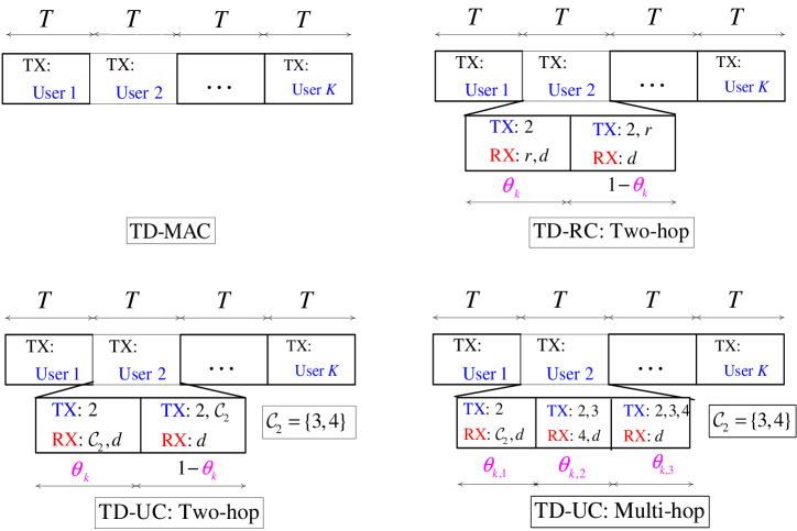
Figure 1: Time-duplexed transmission schemes for the MARC, the MAC-GF, and the MAC.

The relay cooperative (RC) network with $K+1$ inputs $X_{k,i}$, $k\in\mathcal{T}$, and two outputs $Y_{r,i}$ and $Y_{d,i}$ given by (1) is typically modeled as a Gaussian multiaccess relay channel (MARC) [9, 1]. We consider a time-duplexed relay cooperative (TD-RC) model where each source transmits over the channel for a period $T=1/K$ of the total time (see Fig. 1). Further, the transmission period of source $k$, for all $k$, is sub-divided into two slots such that the relay listens in first slot and transmits in the second slot. We denote the time fractions for the two slots as $\theta_{k}$ and $\overline{\theta}_{k}=1-\theta_{k}$ for user $k$ such that $\theta_{k}=\Pr\left(M_{r}=L\right)=1-\Pr\left(M_{r}=T\right)$ where the duration, $\theta_{k}$, of the relay mode $M_{r}$ can be different for different $k$. The time-duplexed two-hop scheme for the RC nework is illustrated in Fig. 1 for user $2$. Also shown is the slot structure for a time-duplexed MAC (TD-MAC). Time-duplexing thus simplifies the analysis for each user to that for a single-source relay channel in each period $T$. We assume that the relay uses negligible resources to communicate its mode transition to the destination. We also assume that, to minimize outage, the transmitters use all available power for transmission subject to (2). Thus, in the $k^{th}$ time period, for all $k$, user $k$ and the relay transmit at power $\overline{P}_{k}=KP_{k}$ and $\overline{P}_{r}=P_{r}/\overline{\theta}_{k}$, respectively, where $\overline{\theta}_{k}=1-\theta_{k}$. Finally, throughout the analysis we assume that $P_{r}$ is proportional to $P_{k}$.

II-C User Cooperative Network

In a user cooperative (UC) network, there is a combinatorial explosion in the number of ways one can duplex $K$ sources over their half-duplex states. We present two transmission schemes that allow each user to be aided by an arbitrary number of users, up to $K-1$. In both schemes the users time-duplex their transmissions; the two schemes differ in the manner the period $T$ is further sub-divided between the transmitting and the cooperating users.

We first consider a two-hop scheme such that the period over which user $k$, for all $k$, transmits is sub-divided into two slots. In the first slot only user $k$ transmits while in the second slot both user $k$ and the set $\mathcal{C}_{k}\subseteq\mathcal{K}\backslash\{k\}$ of users that cooperate with user $k$ transmit. This is shown in Fig. 1 for user $2$ and $\mathcal{C}_{2}=\left\{3,4\right\}$. We remark that this scheme has the same number of hops as the TD-RC network except now user $k$ can be aided by more than one user in $\mathcal{C}_{k}$. We write $\theta_{k}$ and $1-\theta_{k}$ to denote the time fractions associated with the first and second slots of user $k$ such that $\theta_{k}=\Pr\left(M_{j}=L\right)=1-\Pr\left(M_{j}=T\right)$ for all $j\in\mathcal{C}_{k}$.

We also consider a multi-hop scheme where the total transmission time for source $k$ is divided into $L_{k}$ slots, $1\leq L_{k}\leq K$, where $L_{k}=\left|\mathcal{C}_{k}\right|+1$. Specifically, in each time-slot, except the first slot where only user $k$ transmits, one additional user cooperates in the transmission until all $L_{k}$ users transmit in slot $L_{k}$. When the cooperating users decode their received signals, we assume that the users are ordered in the sense that the new user that cooperates in the $l^{th}$ fraction is the first user that can decode the message when the $l$ cooperating users are transmitting. We denote the $l^{th}$ time fraction for user $k$ as $\theta_{k,l}$, $l=1,2,\ldots,L$ (see Fig. 1 for user $2$ with $\mathcal{C}_{2}=\left\{3,4\right\}$). We refer to this model as time-duplexed user cooperation or simply TD-UC.

User $k$ transmits at power

$$\overline{P}_{k}=P_{k}\cdot K\left/\left(N_{k}+1\right)\right.$$ (3)

where $N_{k}\leq K-1$ is the total number of users whose messages are forwarded by user $k$. Further, for the two-hop scheme, in those sub-slots where user $k$ acts as a cooperating node, its transmission power is scaled by the appropriate $\overline{\theta}_{k}$. The energy consumed in every cooperative slot is therefore exactly given by (3). Let $\pi_{k}\left(\cdot\right)$ be a permutation on $\mathcal{C}_{k}$ such that user $\pi_{k}\left(l\right)$ begins its transmissions in the fraction $\theta_{k,l}$, for all $l=2,3,\ldots,L_{k}$, and $\pi_{k}\left(1\right)=k$. Thus, when user $k$ acts as a cooperating node for user $j$, $j\not=k$, such that $\pi_{j}(l)=k$ for some $l>1$, its power $\overline{P}_{k}$ in (3) is scaled by the total fraction for which it transmits for user $j$, i.e., ${\textstyle\sum\nolimits_{m=l}^{L_{j}}}\theta_{j,m}$. We assume that a cooperating node or relay uses negligible resources to communicate its transition from one mode to another to the destination as well as other cooperating nodes. For AF we assume equal length slots and consider symbol-based two-hop and multi-hop schemes.

Finally, throughout the sequel, we assume that due to lack of CSI at the transmitters, the transmitters do not vary power as a function of channel states. Furthermore, each user uses independent Gaussian in each transmitting fraction. Thus, for e.g., for two-hop TD-RC and TD-UC networks under AF, user $k$ transmits independent codebooks with the same power in the two fractions. Similarly, for the multi-hop TD-UC network under AF, subject to (3), user $k$ transmits independent signals with the same power in all $L_{k}$ fractions.

II-D Cost Metric: Total Power

We use the total power consumed by all the nodes as a cost metric for comparisons. Observe that in addition to its transmit power a node also consumes processing power, i.e., in encoding and decoding its transmissions and receptions, respectively. Further, in addition to its own transmission and processing costs, a node that relays consumes additional power in encoding and decoding packets for other nodes. We model these costs by defining encoding and decoding variables $\eta_{k}$ and $\delta_{k}$, respectively, and write the power required to process the transmissions of node $j$ at node $k$ as

$$\begin{array}[c]{cc}P_{k,j}^{proc}=P_{k,0}^{proc}+\left(\eta_{k}I_{k}^{enc}\left(j\right)+\delta_{k}I_{k}^{dec}\left(j\right)\right)\cdot f\left(R_{j}\right)&\text{for all }k\in\mathcal{T},j\in\mathcal{K}\end{array}$$ (4)

where $P_{k,j}^{proc}$ is the power required by user $k$ to cooperate with user $j$, $I_{k}^{enc}\left(j\right)$ and $I_{k}^{dec}\left(j\right)$ are indicator functions that are set to $1$ if user $k$ encodes and decodes, respectively, for user $j$, $P_{k,0}^{proc}$ is the minimum processing power at user $k$ which is in general device and protocol dependent, and $f(R_{j})$ is a function of the transmission rate $R_{j}$ in bits/sec at user $j$. The unitless variables $\eta_{k}$ and $\delta_{k}$ quantify the ratio of processing to transmission power at user $k$ to encode and decode a bit, respectively. For example, a relay node that uses DDF consumes power for overhead, encoding, and decoding costs while a relay node using AF only has overhead costs. Note that for the relay node, we have $P_{r,r}^{proc}=P_{r,0}^{proc}$ which accounts for the costs of simply operating the relay. Thus, for the examples in Section I, we have $\eta<1$ and $\delta<1$ for the RAZR phone, $\eta>>1$ and $\delta>>1$ for the Atheros LAN card, and $\eta$ and $\delta$ determined by the cross-over distance for the Berkeley motes. In general, the processing cost function $f$ depends on the encoding and decoding schemes used as well as the device functionality. For simplicity, we choose $f$ as

$$\begin{array}[c]{cc}f\left(R_{k}\right)=R_{k}&\text{for all }k.\end{array}$$ (5)

Finally, we assume that the destination in typical multiaccess networks such as cellular or many-to-one sensor networks has access to an unlimited energy source and ignore its processing costs. We write the total power consumed on average (over all channel uses) at node $k$, $k\in\mathcal{T}$, as

$$P_{k,tot}=\left\{\begin{array}[c]{ll}P_{k}+P_{k,k}^{proc}+\sum\limits_{j\in\mathcal{K},j\not=k}I_{k}(j)P_{k,j}^{proc}&k\in\mathcal{K}\\ P_{k}+\sum\limits_{j\in\mathcal{K}}I_{k}(j)P_{k,j}^{proc}&k=r\end{array}\right.$$ (6)

where $I_{k}(j)$ is an indicator function that takes the value $1$ if node $k$ cooperates with node $j$. For user $k,$ the first $P_{k,k}^{proc}$ term in (6) corresponds to the power used to process its own message while the second summation term accounts for the power node $k$ incurs in cooperating with all other source nodes. Note that at high SNR, i.e., high $P_{k}$ for all $k$, the dominating term in (6) is $P_{k}$ since $P_{k,0}^{proc}$ is usually a constant and $R_{j}$ increases logarithmically in $P_{j}$, for all $k,j\in\mathcal{K}$. The total power consumed by all transmitting nodes in each network is given as

$$P_{tot}=\left\{\begin{array}[c]{ll}\sum\limits_{k\in\mathcal{K}}P_{k,tot}&\text{TD-MAC\ or UC}\\ \sum\limits_{k\in\mathcal{T}}P_{k,tot}&\text{RC.}\end{array}\right.$$ (7)

II-E Fading Models

We model the fading gains as $H_{m,k,i}=A_{m,k,i}\left/d_{m,k}^{\gamma/2}\right.$ where $d_{m,k}$ is the distance between the $m^{th}$ receiver and the $k^{th}$ source, $\gamma$ is the path-loss exponent, and the $A_{m,k,i}$ are jointly independent identically distributed (i.i.d.) zero-mean, unit variance proper, complex Gaussian random variables. We assume that the fading gain $H_{m,k,i}$ is known only at receiver $m$. We also assume that $H_{k,m,i}$ remains constant over a coherence interval and changes independently from one coherence interval to another. Further, the coherence interval is assumed large enough to transmit a codeword from any transmitter and all its cooperating nodes or relay. Finally, we also assume that the fading gains are independent of each other and independent of the transmitted signals $X_{k,i}$, for all $k\in\mathcal{T}$ and $i$.

III Geometry-inclusive Outage Analysis

We compare the outage performance of the user and relay cooperative networks via a limiting analysis in SNR of the outage probabilities achieved by DDF and AF. Such an analysis enables the characterization of two key parameters, namely, the diversity order and the coding gains, which correspond to the slope and the SNR intercept, respectively, of the log-outage vs. SNR in dB curve [6]. In [6], Laneman develops bounds on the DF and AF outage probabilities for a relay channel where the source and the relay transmit on orthogonal channels. In [5], the authors introduce a DDF strategy where the cooperating node/relay remains in the listen mode until it successfully decodes its received signal from the source. The authors show that, for both two-hop and multi-hop relay channels, DDF achieves the diversity-multiplexing tradeoff (DMT) performance [10] of an equivalent MIMO channel for small multiplexing gains. In an effort to quantify the diversity and the effect of geometry, we present geometry-inclusive upper and lower bounds on the DDF and AF outage probability for TD-RC and two-hop and multi-hop TD-UC networks. We summarize the results here and develop the detailed analyses in the Appendices.

III-A Dynamic-Decode-and-Forward

III-A1 TD-RC

In general, obtaining a closed form expression for the outage probability of each user is not straightforward. Suppose that $P_{r}=\lambda\overline{P}_{k}$ for some constant $\lambda$ and recall that $\overline{P}_{r}=\left.P_{r}\right/\overline{\theta}_{k}$. In Appendix B, we develop upper and lower bounds on the DDF outage probability $P_{o}^{(k)}$ of user $k$ transmitting at a fixed rate $R_{k}$, for all $k$, as

$$P_{o,2\times 1}\leq P_{o}^{(k)}\leq\left[\frac{(2^{R_{k}/\overline{\theta}_{k}^{\ast}}-1)^{2}\overline{\theta}_{k}^{\ast}}{(2^{R_{k}}-1)^{2}}+\frac{2d_{r,k}^{\gamma}(2^{R_{k}/\theta_{k}^{\ast}}-1)^{2}}{d_{d,r}^{\gamma}(2^{R_{k}}-1)^{2}}\right]\cdot\frac{(2^{R}-1)^{2}d_{d,k}^{\gamma}d_{d,r}^{\gamma}}{2\lambda\overline{P}_{k}^{2}}+O\left(\overline{P}_{k}^{-3}\right)$$ (8)

where $P_{o,2\times 1}$ is the outage probability of a $2\times 1$ distributed MIMO channel whose $i^{th}$ transmit antenna is at a distance $d_{d,i}$, $i=k,r$, from the destination and $\theta_{k}^{\ast}\in\left(0,1\right)$ is a fraction chosen to upper bound $P_{o}^{\left(k\right)}$. The notation $O\left(x\right)$ in (8) means that there is a positive constant $M$ such that the $O\left(x\right)$ term is upper bounded by $M\left|x\right|$ for all $x\geq x_{0}$. In Appendix B, we show that

$$P_{o,2\times 1}=(2^{R_{k}}-1)^{2}d_{d,k}^{\gamma}d_{d,r}^{\gamma}\left/2\overline{\lambda P}_{k}^{2}\right.+O\left(\overline{P}_{k}^{-3}\right).$$ (9)

Thus, from (8) and (9) we see that for a fixed rate transmission, the maximum diversity achieved by DDF is $2$, as predicted by the DMT analysis for DDF in [5, Theorem 4]. Comparing (8) and (9), we further see that the bracketed expressions on the right side of the inequality in (8) upper bounds the coding gains by which $P_{o}^{(k)}$ differs from the MIMO lower bounds.

III-A2 TD-UC – Two-Hop

The outage analysis for the two-hop TD-RC network can be extended to the two-hop TD-UC network. In Appendix B, for sufficiently large power $P_{k}$, we bound $P_{o}^{(k)}$ as (see 55) and (61))

$$P_{o,L_{k}\times 1}\leq P_{o}^{(k)}\leq K_{2}\cdot\frac{\left(2^{R_{k}}-1\right)^{L_{k}}\prod_{j\in\mathcal{S}_{k}}d_{d,j}^{\gamma}}{\left(L_{k}!\right)\left(\overline{P}_{k}\right)^{L_{k}}\prod\limits_{j\in\mathcal{S}_{k}}\lambda_{j}}+O\left(\overline{P}_{k}^{-L_{k}-1}\right)$$ (10)

where $\lambda_{j}=\overline{P}_{j}/\overline{P}_{k}$ for all $j\in\mathcal{S}_{k}=\mathcal{C}_{k}\cup\left\{k\right\}$, $\theta_{k}^{\ast}\in\left(0,1\right)$, $P_{o,L_{k}\times 1}$ is the outage probability of a $L_{k}\times 1$ distributed MIMO channel whose $i^{th}$ transmit antenna is at a distance $d_{d,i}$, $i=1,2,\ldots,L_{k}$, from the destination such that

$$P_{o,L_{k}\times 1}=\frac{\left(2^{R_{k}}-1\right)^{L_{k}}}{\left(L_{k}!\right)\left(\overline{P}_{k}\right)^{L_{k}}}\prod_{j\in\mathcal{S}_{k}}\frac{d_{d,j}^{\gamma}}{\lambda_{j}}+O\left(\overline{P}_{k}^{-L_{k}-1}\right)$$ (11)

and

$$K_{2}=\left[\frac{\left(2^{R_{k}/\overline{\theta}_{k}^{\ast}}-1\right)^{L_{k}}\left(\overline{\theta}_{k}^{\ast}\right)^{L_{k}-1}}{\left(2^{R_{k}}-1\right)^{L_{k}}}+\frac{(2^{R_{k}/\theta_{k}^{\ast}}-1)^{2}\left(\sum_{j\in C_{k}}d_{j,k}^{\gamma}\right)\left(L_{k}!\right)\left(\overline{P}_{k}\right)^{L_{k}-2}}{\left(2^{R_{k}}-1\right)^{L_{k}}\left(\prod_{j\in\mathcal{C}_{k}}d_{d,j}^{\gamma}/\lambda_{j}\right)}\right].$$ (12)

Note that for $L_{k}=2$, our analysis simplifies to the outage analysis for the TD-RC network. For $L_{k}>2$, comparing the two terms in the right-hand sum in (12), we see that a lower bound on the diversity from the first and second terms are $L_{k}$ and $2$, respectively. In fact, the first term dominates only when

$$\left(\sum_{j\in C_{k}}d_{j,k}^{\gamma}\right)\leq\frac{\left(2^{R_{k}/\overline{\theta}_{k}^{\ast}}-1\right)^{L_{k}-2}}{\left(L_{k}!\right)\left(\overline{P}_{k}\right)^{L_{k}-2}}\cdot\frac{\left(\prod_{j\in\mathcal{S}_{k}}d_{d,j}^{\gamma}/\lambda_{j}\right)}{d_{d,k}^{\gamma}}.$$ (13)

Thus, for a given $P_{k}$, for all $k$, achieving the maximum diversity $L_{k}$ requires that user $k$ and its cooperating users in $\mathcal{C}_{k}$ are clustered close enough to satisfy (13). Thus, the maximum DDF diversity for a two-hop cooperative network does not exceed that of TD-RC except when user $k$ and its cooperating users are clustered, i.e., the inter-node distances satisfy (13). We illustrate this distance-dependent behavior in Section IV.

III-A3 TD-UC – Multi-Hop

Recall that $\pi_{k}\left(\cdot\right)$ is a permutation on $\mathcal{C}_{k}$ such that user $\pi_{k}\left(l\right)$ begins its transmissions in the fraction $\Theta_{k,l}$, for all $l=2,3,\ldots,L_{k}$, and $\pi_{k}\left(1\right)=k$. Unlike the two-hop case where $\Theta_{k}$ is dictated by the node with the worst receive SNR, the fraction $\Theta_{k,l}$, for $l=1,2,\ldots,L_{k}-1$, is the smallest fraction that ensures that at least one cooperating node, denoted as $\pi_{k}\left(l+1\right)$, decodes the message from user $k$. In general, developing closed form expressions for $P_{o}^{(k)}$ is not straightforward. In Appendix C, we lower bound $P_{o}^{\left(k\right)}$ by the MIMO outage probability, $P_{o,L_{k}\times 1}$ and use the CDF of $\Theta_{k,l}$, for all $l$, to upper bound $P_{o}^{\left(k\right)}$ for any $0<\theta_{k,l}^{\ast}<1$, for all $l$, as (see (76))

$$P_{o}^{\left(k\right)}\leq\frac{\left(2^{R_{k}}-1\right)^{L_{k}}}{\left(L_{k}!\right)\left(\overline{P}_{k}\right)^{L_{k}}}\left(\prod_{j=1}^{L_{k}}\frac{d_{d,\pi_{k}\left(j\right)}^{\gamma}}{\lambda_{\pi_{k}\left(j\right)}}\right)\cdot\left[K_{c}+K_{d}\right]+O\left(\overline{P}_{k}^{-L_{k}-1}\right)$$ (14)

where the constants $K_{c}$ and $K_{d}$ are given by (77) in Appendix C. Our analysis shows that DDF achieves a maximum diversity of $L_{k}$ for a $L_{k}$-hop TD-UC network.

III-B Amplify-and-Forward

A cooperating node or a relay can amplify its received signal and forward it to the destination; the resulting AF strategy is appropriate for nodes with limited processing capabilities. We present the outage bounds for the two-hop TD-RC and TD-UC and the $L_{k}$-hop TD-UC networks. We assume $\theta_{k}=1/2$ and $\theta_{k,l}=1/L_{k}$, $l=1,2,\ldots,L_{k}$, for the two-hop and $L_{k}$-hop schemes, respectively.

III-B1 TD-RC and TD-UC – Two-hop

We first consider a two-hop AF protocol where only user $k$ transmits in the first fraction and both user $k$ and its cooperating users (TD-UC) or relay (TD-RC) transmit in the second fraction. User $k$ transmits with a different codebook in the first and second fractions. The outage analysis for the two-hop TD-RC network, i.e., $\left|\mathcal{C}_{k}\right|=1$, is the same as that developed for the half-duplex relay channel in [11]. Recall that due to lack of transmit CSI, we assume no power control and independent Gaussian codebooks in each transmit fraction at user $k,$ for all $k$. For the TD-UC network, i.e., $L_{k}\geq 2$, where all $L_{k}-1$ cooperating nodes amplify and forward their received signals in the second fraction, the received and transmitted signals $\left(Y_{d,1},Y_{d,2}\right)$ and $\left(X_{k,1},X_{k,2}\right)$, respectively, in the two fractions are

$$\begin{bmatrix}Y_{d,1}\\ Y_{d,2}\end{bmatrix}=\begin{bmatrix}H_{d,k}&0\\ \sum\limits_{j\in\mathcal{C}_{k}}c_{j}H_{d,j}H_{j,k}&H_{d,k}\end{bmatrix}\begin{bmatrix}X_{k,1}\\ X_{k,2}\end{bmatrix}+\begin{bmatrix}Z_{d,1}\\ Z_{d,2}^{\prime}\end{bmatrix}$$ (15)

where

$$\left|c_{j}\right| =\left(2\overline{P}_{j}/\left/\left|H_{j,k}\right|^{2}\overline{P}_{k}+1\right.\right)^{1/2}$$ (16)

$$Z_{d,2}^{\prime} =\left({\textstyle\sum\nolimits_{j\in\mathcal{C}_{k}}}c_{j}H_{d,j}Z_{j,k}\right)+Z_{d,2}$$ (17)

$$c_{s}^{2} =1+\sum\nolimits_{j\in\mathcal{C}_{k}}\left|c_{j}H_{d,j}\right|^{2}.$$ (18)

and $Z_{j,k}$, $Z_{d,1}$, and $Z_{d,2}$ are i.i.d. Gaussian noise variables. Scaling $Y_{d,2}$ by $c_{s}$ to set $E\left[\left|Z_{d,2}^{\prime}\right|^{2}\right]=1$, the outage $P_{o}^{(k)}$ is given as

$$P_{o}^{(k)}=\Pr\left(\frac{1}{2}C\left(\left|H_{d,k}\right|^{2}\overline{P}_{k}\left(1+\frac{1}{c_{s}}\right)+\frac{\overline{P}_{k}}{c_{s}^{2}}\left|\sum\limits_{j\in\mathcal{C}_{k}}\frac{c_{j}}{c_{s}}H_{d,j}H_{j,k}\right|^{2}\right)<R_{k}\right)$$ (19)

where the pre-log factor of $1/2$ is a result of $\theta_{k}=1/2$. For $\left|\mathcal{C}_{k}\right|>1$, the terms in (19) with cross products $H_{d,j}H_{j,k}$ may not add constructively. Accordingly, we lower bound $P_{o}^{(k)}$ by the outage probability of a $L_{k}\times 1$ MIMO channel where all but one of the antennas transmit the same signal, i.e.,

$$P_{o}^{(k)}\geq\Pr\left(C\left(\left|H_{d,k}\right|^{2}\overline{P}_{k}+\overline{P}_{k}\left|{\textstyle\sum\nolimits_{j\in\mathcal{C}_{k}}}H_{d,j}\right|^{2}\right)<R_{k}\right)=\frac{\left(2^{R_{k}}-1\right)^{2}d_{d,k}^{\gamma}}{2\overline{P}_{k}^{2}\left(\sum_{j\in\mathcal{C}_{k}}1/d_{d,j}^{\gamma}\right)}+O\left(\overline{P}_{k}^{-3}\right).$$ (20)

Thus, the maximum diversity of two-hop AF is bounded by $2$. Further, since AF achieves a maximum diversity of $2$ with one cooperating node or relay [6], allowing selection of one cooperating node with the smallest outage, we can upper bound $P_{o}^{(k)}$ by the AF outage probability of a relay channel with $\left|\mathcal{C}_{j}\right|=1$. Finally, using the fact that $P_{o}^{(k)}$ for a non-orthogonal relay channel is at most that for the orthogonal relay channel, we apply the high SNR (no CSI at transmitters) bound developed for the latter in [6] to bound $P_{o}^{(k)}$ as

$$P_{o}^{(k)}\leq\frac{\left(2^{2R_{k}}-1\right)^{2}d_{d,k}^{\gamma}\max_{j\in\mathcal{C}_{k}}\left(d_{j,k}^{\gamma}+d_{d,j}^{\gamma}\right)}{2\overline{P}_{k}^{2}}.$$ (21)

Thus, we see that the maximum diversity achievable by a two-hop AF scheme in the high SNR regime is at most $2$ and is independent of the number of cooperating users in $\mathcal{C}_{k}$.

III-B2 TD-UC – Multi-hop

We consider an $L_{k}$-hop cooperative AF protocol where only user $k$ and user $\pi_{k}\left(l\right)$, $l=1,2,\ldots,L_{k}$, transmit in the $l^{th}$ fraction, i.e., user $\pi_{k}\left(l\right)$ forwards in the fraction $\theta_{k,l}$ a scaled version of the signal it receives from user $k$ in the first fraction. User $k$ transmits with a different codebook in the first and second fractions. Note that $\pi_{k}\left(1\right)=k$ and $\theta_{k,l}=1/L_{k}$ for all $l$. We write the received signal, $Y_{d,l}$, at the destination in the $l^{th}$ fraction as

$$Y_{d,l}=\left\{\begin{array}[c]{ll}H_{d,k}X_{k,l}+Z_{d,l}&l=1\\ H_{d,k}X_{k,l}+H_{d,\pi_{k}\left(l\right)}X_{\pi_{k}\left(l\right),l}+Z_{d,l}^{\prime}&l=2,\ldots,L_{k}\end{array}\right.$$ (22)

where the signal transmitted by user $\pi_{k}\left(l\right)$ in the $l^{th}$ fraction is $X_{\pi_{k}\left(l\right),l}=c_{\pi_{k}\left(l\right)}Y_{\pi_{k}\left(l\right),1}=c_{\pi_{k}\left(l\right)}\left(H_{\pi_{k}\left(l\right),k}X_{k,1}+Z_{\pi_{k}\left(l\right),1}\right),$ and $c_{\pi_{k}\left(l\right)}$, $c_{s,\pi_{k}\left(l\right)}^{2}$, and $Z_{d,l}^{\prime}$ are given by (16)-(17), respectively, with $\mathcal{C}_{k}=$ $\left\{\pi_{k}\left(l\right)\right\}$. Similar to (15), (22) can also be written compactly as $Y$${}_{d}=\mathbf{H}\underline{X}_{k}+\underline{Z},$ where the $L_{k}$ entries of $Y$_d and $X$_k are related by (22) and $\mathbf{H}$ is the resulting channel gains matrix. The destination decodes after collecting the received signals from all $L_{k}$ fractions. Choosing $X_{k,l}$, for all $l$, as independent Gaussian signals, we have

$$P_{o}^{(k)}=\Pr\left(\log\left|I+\overline{P}_{k}\mathbf{HH}^{{\dagger}}\right|<L_{k}R_{k}\right)$$ (23)

where $\mathbf{H}^{{\dagger}}$ is the conjugate transpose of $\mathbf{H}$. We lower bound $P_{o}^{(k)}$ with the outage probability of a $L_{k}\times 1$ MIMO channel with i.i.d. Gaussian signaling at the $L_{k}$ transmit antennas to obtain

$$P_{o}^{(k)}\geq P_{o,L_{k}\times 1}=\frac{\left(2^{R_{k}}-1\right)^{L_{k}}\prod_{l=1}^{L_{k}}d_{d,\pi_{k}\left(l\right)}^{\gamma}}{\left(L_{k}!\right)\overline{P}_{k}^{L_{k}}}+O\left(\overline{P}_{k}^{-L_{k}-1}\right).$$ (24)

On the other hand, one can upper bound $P_{o}^{(k)}$ by the outage probability of an orthogonal AF protocol where user $k$ and its cooperating users transmit on orthogonal channels, i.e., only user $\pi_{k}\left(l\right)$ transmits in the fraction $\theta_{k,l}$, as developed in [6]. Thus, we have

$$P_{out}\leq\frac{\left(2^{L_{k}R_{k}}-1\right)^{L_{k}}d_{d,k}^{\gamma}\prod_{j\in\mathcal{C}_{k}}\left(d_{d,j}^{\gamma}+d_{j,k}^{\gamma}\right)}{L_{k}!\overline{P}_{k}^{L_{k}}}.$$ (25)

Comparing (24) and (25), we see that the $L_{k}$-hop AF scheme can achieve a maximum diversity of $L_{k}$ in the high SNR regime at the expense of user $k$ repeating the signal $L_{k}$ times.

IV Illustration of Results

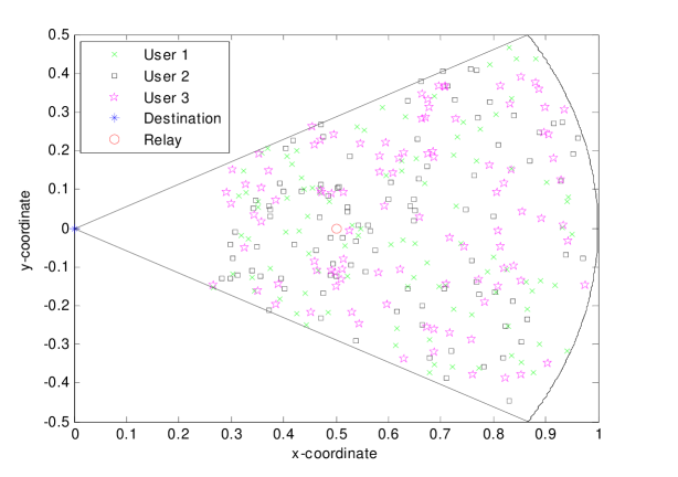
Figure 2: Sector of a circle with the destination at the origin and 100 randomly chosen locations for a three-user MAC.

We consider a planar geometry with the users distributed randomly in a sector of a circle of unit radius and angle $\pi/3$. We place the destination at the center of the circle and place the relay at $(0.5,0)$ as shown in Fig. 2. The $K$ users are distributed randomly over the sector excluding an area of radius $0.3$ around the destination. We consider $100$ such random placements and for each such random placement, we compute the outage probabilities $P_{out}$ for the TD-RC, the TD-UC, and the TD-MAC network as an average over the outages of all the time-duplexed users in each network. Finally, we also average $P_{out}$ over the 100 random node placements. We consider a three-user MAC. We assume that all three users have the same transmit power constraint, i.e., $P_{k}=P_{1}$ for all $k$. For the relay we choose $P_{r}=f_{r}\cdot P_{1}$ where $f_{r}\in\{0.5,1\}$. We set the path loss exponent $\gamma=4$ and the processing factors $\eta_{k}=\delta_{k}=\eta$ for all $k$. We plot $P_{out}$ as a function of $P_{tot}$ for $\eta=0.01,$ $0.5,$ and $1$ thereby modeling three different regimes of processing to transmit power ratios. We consider a symmetric transmission rate, i.e., all users transmit at $R=0.25$ bits/channel use. We first plot $P_{out}$ as a function of the transmit SNR $P_{1}$ in dB obtained by normalizing $P_{1}$ by the unit variance noise. We also plot $P_{out}$ as a function of $P_{tot}$ in dB where $P_{tot}$ is given by (6) and (7). For user cooperation, we plot the outage for both the two-hop and three-hop schemes.

IV-A Outage Probability: DDF

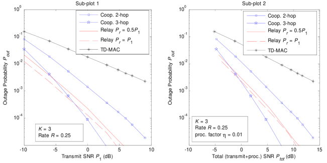
Figure 3: Three user DDF outage probability $P_{out}$ vs. $P_{1}$ (sub-plot 1) and vs. $P_{tot}$ for $\eta=0.01$ (sub-plot 2).

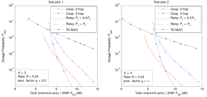
Figure 4: Three user DDF outage probability $P_{out}$ vs. total transmit SNR $P_{tot}$ in dB for $\eta=0.5$ (sub-plot 1) and $\eta=1$ (sub-plot 2).

We compare the outage probability of a three user MAC in Figs. 3 and 4. The plots clearly validate our analytical results that DDF does not achieve the maximum diversity gains of $3$ for the two hop TD-UC network (denoted Coop. 2-hop in plots). On the other hand, the slope of $P_{out}$ for the three-hop TD-UC network, (denoted Coop. 3-hop) approaches $3$. Further, DDF for this network achieves coding gains relative to the TD-RC network only as the SNR increases. In fact, this difference persists even when the energy costs of cooperation are accounted for in sub-plot 2 and Fig. 4 by plotting $P_{out}$ as a function of $P_{tot}$. This difference in SNR gains between user and relay cooperation is due to the fact that user cooperation increases spatial diversity at the expense of requiring users to share their power for cooperative transmissions. Observe that with increasing $\eta$, the outage curves are translated to the right. In fact, for a fixed $R$, the processing costs increase with increasing $\eta$, and thus, we expect the SNR gains from cooperation to diminish relative to TD-MAC, particularly in the lower SNR regimes of interest. This is demonstrated in Fig. 4.

IV-B Outage Probability: AF

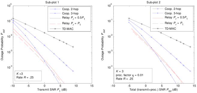
Figure 5: Three user AF outage probability $P_{out}$ vs. $P_{1}$ (sub-plot 1) and $P_{tot}$ for $\eta=0.01$ (sub-plot 2).

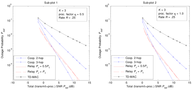
Figure 6: Three user AF outage probability $P_{out}$ vs. $P_{tot}$ for $\eta=0.5$ (sub-plot 1) and $\eta=1$ (sub-plot 2).

In Figs. 5 and 6 we plot the two user AF outage probability for all three networks. As predicted, we see that both TD-RC and TD-UC networks achieve a maximum diversity of $2$ for the two-hop scheme. The three-hop scheme for TD-UC achieves a maximum diversity approaching $3$. However, it achieves coding gains relative to the relay network only as the SNR increases. These gains are a result of the model chosen for the processing power (only model costs of encoding and decoding) and the choice of $P_{k,0}^{proc}=0$ for all $k$ for the purposes of illustration. In general, $P_{k,0}^{proc}>0$ since it models protocol and device overhead including front-end processing and amplification costs, and thus, the total processing power will scale proportionate to the number of users that a node relays for.

The numerical analysis can be extended to arbitrary relay positions [7, Chap. 4]. In general, the choice of relay position is a tradeoff between cooperating with as many users as possible and being, on average, closer than the users are to the destination. To this end, fixing the relay at the symmetric location of $(0.5,0)$ is a reasonable tradeoff.

V Concluding Remarks

We compared the outage performance of user and relay cooperation in a time-duplexed multiaccess network using the total transmit and processing power as a cost metric for the comparison. We developed a model for processing power costs as a function of the transmitted rate. We developed a two-hop cooperation scheme for both the relay and user cooperative network. We also presented a multi-hop scheme for the user cooperative network for the case of multiple cooperating users. We presented geometry-inclusive upper and lower bounds on the outage probability of DDF and AF to facilitate comparisons of diversity and coding gains achieved by the two cooperative approaches. We showed that the TD-RC network achieves a maximum diversity of $2$ for both DDF and AF. We also showed that under a two-hop transmission scheme, a $K$-user TD-UC network achieves a $K$-fold diversity gain with DDF only when the cooperating users are physically proximal and achieves a maximum diversity of $2$ with AF. On the other hand, for a $K$-hop transmission scheme, the TD-UC network achieves a maximum diversity of $K$ for both DDF and AF. Using area-averaged numerical results that account for the costs of cooperation, we demonstrated that the TD-RC network achieves SNR gains that either diminish or completely eliminate the diversity advantage of the TD-UC network in SNR ranges of interest. Besides a fixed relay position, this difference is due to the fact that user cooperation results in a tradeoff between diversity and SNR gains as a result of sharing limited power resources between the users.

In conclusion, we see that user cooperation is desirable only if the processing costs associated with achieving the maximum diversity gains are not prohibitive, i.e., in the regime where user cooperation achieves positive coding gains relative to the relay cooperative and non-cooperative networks. The simple processing cost model presented here captures the effect of transmit rate on processing power. One can also tailor this model to explicitly include delay, complexity, and device-specific processing costs.

Appendix A Distribution of Weighted Sum of Exponential Random Variables

Consider a collection of i.i.d. unit mean exponential random variables $E_{l}$, $l=1,2,\ldots,L$. We denote a weighted sum of $E_{l}$, for all $l$, as $H=\sum_{l=1}^{L}c_{l}E_{l}$ where $c_{l}>0$ and $c_{m}\not=c_{k}$ for all $l$ and $m\not=k$. The following lemma summarizes the probability distribution of $H$ [12, p. 11].

Lemma 1 ([12, p. 11])

The random variable $H$ has a distribution given as

$$p_{H}\left(h\right)=\left\{\begin{array}[c]{ll}\sum_{l=1}^{L}\frac{C_{l}}{c_{l}}e^{-h/c_{l}}&h\geq 0\\ 0&\text{otherwise}\end{array}\right.$$ (26)

where the constants $C_{l}$, for all $l$, are

$$C_{l}=\left\{\begin{array}[c]{ll}1&L=1\\ \frac{\left(-c_{l}\right)^{L-1}}{\prod_{j=1,j\not=l}^{L}\left(c_{j}-c_{l}\right)}&L>1.\end{array}\right.$$ (27)

The cumulative distribution function of $H$ is

$$F_{H}\left(\eta\right)=\sum_{l=1}^{L}C_{l}\left(1-e^{-\eta/c_{l}}\right)$$ (28)

such that the first non-zero term in the Taylor series expansion of $F_{H}\left(\eta\right)$ about $\eta=0$ is $\eta^{L}\left/L!\left(\prod_{l=1}^{L}c_{l}\right)\right.$.

Appendix B DDF Outage Bounds

B-A Two-Hop Relay Cooperative Network

For a DDF relay, the listen fraction is the random variable (see [5, (13), pp. 4157])

$$\Theta_{k}=\min\left(1,R_{k}\left/\log\left(1+\frac{\left|A_{r,k}\right|^{2}\overline{P}_{k}}{d_{r,k}^{\gamma}}\right)\right.\right).$$ (29)

$\Theta_{k}$ is a mixed (discrete and continuous) random variable with a cumulative distribution function (CDF) given as

$$F_{\Theta_{k}}^{(r)}(\theta_{k})=\left\{\begin{array}[c]{ll}0&\theta_{k}\leq 0\\ \exp\left[-\frac{(2^{R_{k}/\theta_{k}}-1)d_{r,k}^{\gamma}}{\overline{P}_{k}}\right]&0<\theta_{k}<1\\ 1&\theta_{k}=1.\end{array}\right.$$ (30)

The mutual information collected at the destination over both the listen and transmit fractions is (see [5, Appendix D])

$$I_{2}^{DF}=\Theta_{k}G_{1}+\overline{\Theta}_{k}G_{2}$$ (31)

where $\overline{\Theta}_{k}=\left(1-\Theta_{k}\right)$, $\overline{P}_{k}=KP_{k}$, $\overline{P}_{r}=P_{r}/\overline{\Theta}_{k}$, and

$$G_{1} =C\left(\left|H_{d,k}\right|^{2}\overline{P}_{k}\right)$$ (32)

$$G_{2} =C\left(\left|H_{d,k}\right|^{2}\overline{P}_{k}+\left|H_{d,r}\right|^{2}\overline{P}_{r}\right).$$ (33)

The outage probability for user $k$ transmitting at a fixed rate $R_{k}$ is then given as

$$P_{o}^{(k)}=\Pr\left(I_{2}^{DF}<R_{k}\right)$$ (34)

From (29), $\Theta_{k}=0$ only for $d_{r,k}=0$, i.e., only when user $k$ and the relay are co-located, and for this case (34) simplifies to the outage probability of a $2\times 1$ MIMO channel given as

$$P_{o,2\times 1}=\Pr\left(C\left(\frac{\left|A_{d,k}\right|^{2}\overline{P}_{k}}{d_{d,k}^{\gamma}}+\frac{\left|A_{d,r}\right|^{2}P_{r}}{d_{d,r}^{\gamma}}\right)<R_{k}\right).$$ (35)

Let $P_{r}$ and $\overline{P}_{k}$ scale such that $P_{r}/\overline{P}_{k}=\lambda$ is a positive constant. Using (28), we have

$$P_{o,2\times 1}=\frac{(2^{R_{k}}-1)^{2}d_{d,k}^{\gamma}d_{d,r}^{\gamma}}{2\lambda\overline{P}_{k}^{2}}+O\left(\overline{P}_{k}^{-3}\right).$$ (36)

$P_{o,2\times 1}$ is a lower bound on $P_{o}^{(k)}$ because $G_{2}\geq G_{1}$. On the other hand, for any $\theta_{k}$ in (31), $P_{o}^{(k)}(\theta_{k})$ can be upper bounded as

$$P_{o}^{(k)}(\theta_{k}) \leq\Pr\left(\theta_{k}G_{1}<R_{k}\right)=P_{o,1}^{(k)}(\theta_{k})$$ (37)

$$P_{o}^{(k)}(\theta_{k}) \leq\Pr\left(\overline{\theta}_{k}G_{2}<R_{k}\right)=P_{o,2}^{(k)}(\theta_{k})$$ (38)

Thus, we have

$$P_{o}^{(k)}=\mathbb{E}P_{o}^{(k)}(\Theta_{k})\leq\mathbb{E}\min(P_{o,1}^{(k)}(\Theta_{k}),P_{o,2}^{(k)}(\Theta_{k}))=P_{UB}^{(k)}$$ (39)

Let

$$\begin{array}[c]{ccc}\eta=2^{R_{k}/\overline{\theta}_{k}}-1,&c_{1}=\frac{\overline{P}_{k}}{d_{d,k}^{\gamma}},&c_{2}=\frac{\overline{P}_{r}}{d_{d,r}^{\gamma}}.\end{array}$$ (40)

From (27), we have $C_{1}=c_{1}\left/\left(c_{1}-c_{2}\right)\right.$ and $C_{2}=c_{2}\left/\left(c_{2}-c_{1}\right)\right.$.

Using Lemma 1, we can expand $P_{o,1}^{(k)}(\theta_{k})$ and $P_{o,2}^{(k)}(\theta_{k})$ in (39) as

$$P_{o,1}^{(k)}(\theta_{k})=\Pr\left(G_{1}<\frac{R_{k}}{\theta_{k}}\right)=1-\exp\left[\frac{-(2^{R_{k}/\theta_{k}}-1)d_{d,k}^{\gamma}}{\overline{P}_{k}}\right]\leq\frac{(2^{R_{k}/\theta_{k}}-1)d_{d,k}^{\gamma}}{\overline{P}_{k}}$$ (41)

$$P_{o,2}^{(k)}(\theta_{k})=\Pr\left(G_{2}<\frac{R_{k}}{\overline{\theta}_{k}}\right)=\sum_{l=1}^{2}C_{l}\left(1-e^{-\eta/c_{l}}\right)=\frac{(2^{R_{k}/\overline{\theta}_{k}}-1)^{2}\overline{\theta}_{k}d_{d,k}^{\gamma}d_{d,r}^{\gamma}}{2\lambda\overline{P}_{k}^{2}}+O\left(\overline{P}_{k}^{-3}\right)$$ (42)

where the bound in (42) follows from expanding and simplifying the exponential functions. From (42), we see that for a fixed $\overline{P}_{k}$ and $d_{j,k}$ for all $j,k$, the minimum in (39) is dominated by $P_{o,2}^{(k)}(\theta_{k})$ for small $\theta_{k}$ and by $P_{o,1}^{(k)}(\theta_{k})$ as $\theta_{k}$ approaches $1$. Finally, we have $P_{o,2\times 1}=P_{o,2}^{(k)}(\theta_{k}=0)$.

In general, $P_{UB}^{(k)}$ is not easy to evaluate analytically. Since we are interested in the achievable diversity, we develop a bound on $P_{UB}^{(k)}$ for a fixed $R_{k}$. We have, for any $\theta_{k}^{\ast}$, $0<\theta_{k}^{\ast}<1$,

$$P_{UB}^{(k)} =\int_{0}^{1}P_{\Theta_{k}}\left(\theta_{k}\right)\min\left(P_{o,1}^{(k)}(\theta_{k}),P_{o,2}^{(k)}(\theta_{k})\right)d\theta_{k}$$ (43)

$$\leq\int_{0}^{\theta_{k}^{\ast}}P_{\Theta_{k}}\left(\theta_{k}\right)P_{o,2}^{(k)}(\theta_{k})d\theta_{k}+\int_{\theta_{k}^{\ast}}^{1}P_{\Theta_{k}}\left(\theta_{k}\right)P_{o,1}^{(k)}(\theta_{k})d\theta_{k}$$ (44)

$$\leq F_{\Theta_{k}}\left(\theta_{k}^{\ast}\right)P_{o,2}^{(k)}(\theta_{k}^{\ast})+\left(1-F_{\Theta_{k}}\left(\theta_{k}^{\ast}\right)\right)P_{o,1}^{(k)}(\theta_{k}^{\ast})$$ (45)

$$\leq P_{o,2}^{(k)}(\theta_{k}^{\ast})+\frac{(2^{R_{k}/\theta_{k}^{\ast}}-1)d_{r,k}^{\gamma}}{\overline{P}_{k}}\cdot P_{o,1}^{(k)}(\theta_{k}^{\ast})$$ (46)

$$\leq\left[\frac{(2^{R_{k}/\overline{\theta}_{k}^{\ast}}-1)^{2}\overline{\theta}_{k}^{\ast}}{(2^{R_{k}}-1)^{2}}+\frac{2d_{r,k}^{\gamma}(2^{R_{k}/\theta_{k}^{\ast}}-1)^{2}\lambda}{d_{d,r}^{\gamma}(2^{R_{k}}-1)^{2}}\right]\cdot\frac{(2^{R_{k}}-1)^{2}d_{d,k}^{\gamma}d_{d,r}^{\gamma}}{2\lambda\overline{P}_{k}^{2}}+O\left(\overline{P}_{k}^{-3}\right)$$ (47)

where the equality in (44) holds when $P_{o,2}^{(k)}(\theta_{k})<P_{o,1}^{(k)}(\theta_{k})$ for $\theta_{k}<\theta_{k}^{\ast}$ and vice-versa, and (45) follows because $P_{o,1}^{(k)}(\theta_{k})$ and $P_{o,2}^{(k)}(\theta_{k})$ decrease and increase, respectively, with $\theta_{k}$ and (46) follows from using (30) to bound $1-F_{\Theta_{k}}\left(\theta_{k}^{\ast}\right)$. Finally, we note that for any fixed $0<\theta_{k}^{\ast}<1$, for fixed inter-node distances, the term in square brackets in (47) is a multiplicative constant separating the upper bound (47) and the lower bound (36) on $P_{o}^{\left(k\right)}$.

B-B Two-hop User Cooperative Network

The above analysis extends to the two-hop TD-UC network. Recall that a DDF cooperating node remains in the listen mode until it successfully decodes its received signal from the source. Thus, for the two-hop TD-UC network, the listen fraction for each cooperating node $j$, for all $j\in\mathcal{C}_{k}$, is given by (29) with the substition $r=j$. Further, since the listen fraction $\Theta_{k}$ is now the largest among all $j$, from (29) we have

$$\Theta_{k}=\min\left(1,\max\nolimits_{j\in\mathcal{C}_{k}}\left\{R_{k}\left/C\left(\left.\left|A_{j,k}\right|^{2}\overline{P}_{k}\right/d_{j,k}^{\gamma}\right)\right.\right\}\right)$$ (48)

where the transmit power $\overline{P}_{k}$, for all $k\in\mathcal{K}$, satisfies (2) and is given by (3). Let $F_{\Theta_{k}}^{(j)}(\theta_{k})$ be the CDF $F_{\Theta_{k}}^{(r)}(\theta_{k})$ in (30) with the index $r$ replaced by $j$. From the independence of $A_{j,k}$ for all $j\in\mathcal{C}_{k}$, the CDF of $\Theta_{k}$ is

$$F_{\Theta_{k}}(\theta_{k})=\prod_{j\in\mathcal{C}_{k}}F_{\Theta_{k}}^{(j)}(\theta_{k})=\left.F_{\Theta_{k}}^{(r)}(\theta_{k})\right|_{d_{r,k}={\textstyle\sum_{j\in C_{k}}}d_{j,k}^{\gamma}}.$$ (49)

The destination collects information from the transmissions of user $k$ and all its cooperating nodes in $\mathcal{C}_{k}$ over both the transmit and listen fractions. The resulting mutual information achieved by user $k$ at the destination is (see [13])

$$I_{2,DF}^{c}(\Theta_{k})=\Theta_{k}G_{1}+\overline{\Theta}_{k}G_{2}$$ (50)

where $\overline{\Theta}_{k}=1-\Theta_{k}$ and

$$G_{1} =C\left(\left|H_{d,k}\right|^{2}\overline{P}_{k}\right)$$ (51)

$$G_{2} =C\left(\left|H_{d,k}\right|^{2}\overline{P}_{k}+\sum_{j\in\mathcal{C}_{k}}\left|H_{d,j}\right|^{2}\frac{\overline{P}_{j}}{\overline{\Theta}_{k}}\right).$$ (52)

The DDF outage probability for user $k$ transmitting at a fixed rate $R_{k}$ in a two-hop TD-UC network is thus given as

$$P_{o}^{(k)}=\Pr\left(I_{2,DF}^{c}<R_{k}\right).$$ (53)

From (48), $\Theta_{k}=0$ only if $d_{j,k}=0$ for all $j\in\mathcal{C}_{k}$.

From (50), we can lower bound $P_{o}^{(k)}$ by the outage probability, $P_{o,L_{k}\times 1}$, of a $L_{k}\times 1$ distributed MIMO channel given as

$$P_{o,L_{k}\times 1}=\Pr\left(C\left(\frac{\left|A_{d,k}\right|^{2}\overline{P}_{k}}{d_{d,k}^{\gamma}}+\sum_{j\in\mathcal{C}_{k}}\frac{\left|A_{d,j}\right|^{2}\overline{P}_{j}}{d_{d,j}^{\gamma}}\right)<R_{k}\right).$$ (54)

We enumerate the $\left(L_{k}-1\right)$ cooperative nodes in $\mathcal{C}_{k}$ as $l=2,3,\ldots,L_{k}$, and write $\mathcal{S}_{k}=\left\{k\right\}\cup\mathcal{C}_{k}$. Using (28), and scaling $\overline{P}_{j}$ and $\overline{P}_{k}$ such that $\overline{P}_{j}/\overline{P}_{k}=$ $\lambda_{j}$ is a constant, for all $j$, we have

$$P_{o,L_{k}\times 1}=\frac{(2^{R_{k}}-1)^{L_{k}}d_{d,k}^{\gamma}}{\left(L_{k}!\right)\overline{P}_{k}^{L_{k}}}\cdot\left(\prod_{j\in\mathcal{S}_{k}}\frac{d_{d,j}^{\gamma}}{\lambda_{j}}\right)+O\left(\overline{P}_{k}^{-L_{k}-1}\right).$$ (55)

Let

$$\begin{array}[c]{ccc}\eta=2^{R_{k}/\overline{\theta}_{k}}-1,&c_{1}=\frac{\overline{P}_{k}}{d_{d,k}^{\gamma}},&\begin{array}[c]{cc}c_{l}=\frac{\overline{P}_{l}}{d_{d,l}^{\gamma}\overline{\theta}_{k}},&l=2,3,\ldots,L_{k}\end{array}\end{array}$$ (56)

where the $\overline{\theta}_{k}$ in $c_{l}$ is due to the definition of $\overline{P}_{l}$ in (3). The $C_{l}$, for all $l=1,2,\ldots,L_{k}$, are given by (27). For a fixed $R_{k}$, we upper bound $P_{o}^{(k)}$ using (37)-(38) as

$$P_{o}^{(k)}=\mathbb{E}P_{o}^{(k)}(\Theta_{k})\leq\mathbb{E}\min(P_{o,1}^{(k)}(\Theta_{k}),P_{o,2}^{(k)}(\Theta_{k}))=P_{UB}^{\left(k\right)}.$$ (57)

We upper bound $P_{o,1}^{(k)}(\theta_{k})$ using (41) and compute

$$P_{o,2}^{(k)}(\theta_{k})=\frac{\left(2^{R_{k}/\overline{\theta}_{k}}-1\right)^{L_{k}}\left(\overline{\theta}_{k}\right)^{L_{k}-1}}{\left(L_{k}!\right)\left(\overline{P}_{k}\right)^{L_{k}}}\left(\prod_{j\in\mathcal{S}_{k}}\frac{d_{d,j}^{\gamma}}{\lambda_{j}}\right)+O\left(\overline{P}_{k}^{-L_{k}-1}\right).$$ (58)

Analogous to the steps in (43)-(47) for the TD-RC case, we have (see (57)), for any $\theta_{k}^{\ast}$, $0<\theta_{k}^{\ast}<1$,

$$P_{UB}^{(k)} \leq F_{\Theta_{k}}\left(\theta_{k}^{\ast}\right)P_{o,2}^{(k)}(\theta_{k}^{\ast})+\left(1-F_{\Theta_{k}}\left(\theta_{k}^{\ast}\right)\right)P_{o,1}^{(k)}(\theta_{k}^{\ast})$$ (59)

$$\leq P_{o,2}^{(k)}(\theta_{k}^{\ast})+\frac{(2^{R_{k}/\theta_{k}^{\ast}}-1)\left(\sum_{j\in C_{k}}d_{j,k}^{\gamma}\right)}{\overline{P}_{k}}\cdot P_{o,1}^{(k)}(\theta_{k}^{\ast})$$ (60)

$$=\left[\frac{(2^{R_{k}/\overline{\theta}_{k}^{\ast}}-1)^{L_{k}}\left(\overline{\theta}_{k}^{\ast}\right)^{L_{k}-1}}{(2^{R_{k}}-1)^{L_{k}}}+\frac{\left(L_{k}!\right)\left(\sum\limits_{j\in\mathcal{C}_{k}}d_{j,k}^{\gamma}\right)\overline{P}_{k}^{L_{k}-2}(2^{R_{k}/\theta_{k}^{\ast}}-1)^{2}}{\left(\prod\nolimits_{j\in\mathcal{C}_{k}}d_{d,j}^{\gamma}/\lambda_{j}\right)(2^{R_{k}}-1)^{L_{k}}}\right]\cdot$$

$$\text{ \ \ }\left[\frac{(2^{R_{k}}-1)^{L_{k}}}{\left(L_{k}!\right)\overline{P}_{k}^{L_{k}}}\left(\prod_{j\in\mathcal{S}_{k}}\frac{d_{d,j}^{\gamma}}{\lambda_{j}}\right)\right]+O\left(\overline{P}_{k}^{-L_{k}-1}\right).$$ (61)

Appendix C Multi-hop Cooperative Network – DDF Outage Analysis

The DDF outage probability of user $k$ transmitting at a fixed rate $R_{k}$ in a multi-hop user cooperative network is

$$P_{o}^{(k)}=\Pr\left(I_{2,DF}^{c}<R_{k}\right)$$ (62)

where

$$I_{2,DF}^{c}(\Theta_{k})=\sum_{l=1}^{L_{k}}\Theta_{k,l}G_{l}\text{.}$$ (63)

The function $G_{l}$ is given by

$$\begin{array}[c]{cc}G_{l}=C\left(\sum_{j=1}^{l}\left|H_{d,\pi_{k}(j)}\right|^{2}\frac{\overline{P}_{\pi_{k}(j)}}{\overline{\Theta}_{k,j}}\right)&l=1,2,\ldots L_{k},\end{array}$$ (64)

where $\overline{P}_{k}$ is given by (3) and

$$\begin{array}[c]{cc}\Theta_{k,l}^{sum}\overset{\vartriangle}{=}\sum_{j=1}^{l-1}\Theta_{k,j}&\text{for }l=1,2,\ldots,L_{k}\end{array}$$ (66)

$$\begin{array}[c]{cc}\overline{\Theta}_{k,l}^{sum}\overset{\vartriangle}{=}1-\Theta_{k,l}^{sum}&\end{array}$$ (68)

with $\overline{\Theta}_{k,L_{k}}^{sum}=\Theta_{k,L_{k}}$ and $\Theta_{k,-1}=0$ such that $\overline{\Theta}_{k,1}^{sum}=1$. Recall that $\pi_{k}\left(\cdot\right)$ is a permutation on $\mathcal{C}_{k}$ such that user $\pi_{k}\left(l\right)$ begins its transmissions in the fraction $\Theta_{k,l}$, for all $l=2,3,\ldots,L_{k}$. Furthermore, $\pi_{k}\left(1\right)=k$ and we write $\pi_{k}\left(i:j\right)=\{\pi_{k}(i),$ $\pi_{k}(i+1),$ $\ldots,$ $\pi_{k}(j)\}$.

We write $\underline{\Theta}_{k}$ to denote a $\left(L_{k}-1\right)$-length random vector with entries $\Theta_{k,l}$, $l=1,2,\ldots,L_{k}-1$, and $\lambda_{\pi_{k}\left(j\right)}=\overline{P}_{\pi_{k}\left(j\right)}/\overline{P}_{k}$ for all $\pi_{k}\left(j\right)\in\mathcal{C}_{k}$. Further, we write $\underline{\Theta}_{k}^{\left(l\right)}$ to denote the vector of the first $l$ entries of $\underline{\Theta}_{k}$. The fraction $\Theta_{k,l}$, $l=1,2,\ldots,L_{k}-1$, is the smallest value such that at least one new node, denoted as $\pi_{k}\left(l+1\right)$, decodes the message from user $k$. The analysis for this problem seems difficult; so we replace it by analyzing a simpler strategy where node $\pi_{k}\left(l+1\right)$ collects energy only in fraction $\Theta_{k,l}$ from the transmissions of user $k$ as well as the users in $\pi_{k}\left(1:l\right)$. For this strategy, we have

$$\Theta_{k,l}=\min\left\{\overline{\Theta}_{k,l}^{sum},\min_{\pi_{k}\left(l+1\right)\in\mathcal{C}_{k}\backslash\pi_{k}\left(1:l\right)}\frac{R_{k}}{C\left(\sum_{m=1}^{l}\left.\left|A_{\pi_{k}\left(l+1\right),\pi_{k}(m)}\right|^{2}\overline{P}_{\pi_{k}(m)}\right/d_{\pi_{k}\left(l+1\right),\pi_{k}(m)}^{\gamma}\right)}\right\}.$$ (69)

Applying Lemma 1, the CDF of $\Theta_{k,l}$ conditioned on $\Theta$${}_{k}^{l-1}=\underline{\theta}_{k}^{l-1}$ simplifies to

$$F_{\Theta_{k,l}|\underline{\Theta}_{k,1}^{l-1}}(\theta_{k,l}|\underline{\theta}_{k}^{l-1})=\left\{\begin{array}[c]{ll}0&\theta_{k,l}\leq 0\\ 1-\prod\nolimits_{j\in\mathcal{C}_{k}\backslash\pi_{k}\left(2:l\right)}\left[F_{H_{j,l}^{sum}}(2^{R_{k}/\theta_{k,l}}-1)\right]&0<\theta_{k,l}<\overline{\theta}_{k,l}^{sum}\\ 1&\theta_{k,l}=\overline{\theta}_{k,l}^{sum}.\end{array}\right.$$ (70)

where from (69), $H_{j,l}^{sum}\overset{\vartriangle}{=}\sum_{m=1}^{l}c_{m}\left|A_{j,\pi_{k}(m)}\right|^{2}$ with $c_{m}=\left.\lambda_{\pi_{k}\left(m\right)}\overline{P}_{k}\right/d_{j,\pi_{k}(m)}^{\gamma}$ for all $m=1,2,\ldots,l$, and $\overline{\theta}_{k,l}$ is given by (66). The dominant term of each $F_{H_{j,l}^{sum}}$ is proportional to $\overline{P}_{k}^{-l}$, and thus, the dominant term of $1-F_{\Theta_{k,l}|\underline{\Theta}_{k}^{l-1}}$ is proportional to $\overline{P}_{k}^{-l\left(L_{k}-l\right)}$.

For a fixed $R_{k}$, we lower bound $P_{o}^{(k)}$ by the outage probability $P_{o,L_{k}\times 1}$ of a $L_{k}\times 1$ distributed MIMO channel in (55). Generalizing the analyses in Appendix B, we upper bound $P_{o}^{(k)}$ as (see (62) and (63))

$$P_{o}^{(k)}\leq\mathbb{E}\min_{l\in\mathcal{K}}(P_{o,l}^{(k)}(\underline{\Theta}_{k}))=P_{UB}^{(k)}$$ (71)

where we use Lemma 1 to write

$$P_{o,l}^{(k)}(\underline{\theta}_{k})\overset{\vartriangle}{=}\Pr\left(G_{l}<\frac{R_{k}}{\theta_{k,l}}\right)=\frac{\left(2^{R_{k}/\theta_{k,l}}-1\right)^{l}}{\left(l!\right)\left(\overline{P}_{k}\right)^{l}}\left(\prod_{j=1}^{l}\frac{d_{d,\pi_{k}\left(j\right)}^{\gamma}\overline{\theta}_{k,j}^{sum}}{\lambda_{\pi_{k}\left(j\right)}}\right)+O\left(\overline{P}_{k}^{-l-1}\right).$$ (72)

The probability $P_{UB}^{(k)}$ is given as (see (62) and (66))

$$P_{UB}^{(k)}=\int_{\theta_{k,1}=0}^{1}\int_{\theta_{k,2}=0}^{\overline{\theta}_{k,2}^{sum}}\ldots\int_{\theta_{k,L_{k}-1}=0}^{\overline{\theta}_{k,L_{k}-1}^{sum}}P_{\underline{\Theta}_{k}}\left(\underline{\theta}_{k}\right)\min_{l\in\mathcal{K}}(P_{o,l}^{(k)}(\theta_{k,l}))d\theta_{k}.$$ (73)

For any $0<\theta_{k,l}^{\ast}<\overline{\theta}_{k,l}^{\ast}$, $1\leq l<L_{k}$, the integral in (73) over the $\left(L_{k}-1\right)$-dimensional hyper-cube can be written as a sum of $2^{L_{k}-1}$ integrals, each spanning $\left(L_{k}-1\right)$-dimensions, such that there are $\tbinom{L_{k}-1}{j}$ integrals for which $j$ of the $\left(L_{k}-1\right)$ $\theta_{k,l}$ parameters range from $0$ to $\theta_{k,l}^{\ast}$, $j=0,1,\ldots,L_{k}-1$ while the remaining range from $\theta_{k,l}^{\ast}$ to $1$. Thus, we upper bound $P_{UB}^{(k)}$ in (73) by

$$\int_{0}^{\theta_{k,1}^{\ast}}\int_{0}^{\overline{\theta}_{k,2}^{sum}}\ldots\int_{0}^{\overline{\theta}_{k,L_{k}-1}^{sum}}P_{\underline{\Theta}_{k}}\left(\underline{\theta}_{k}\right)P_{o,L_{k}}^{(k)}(\underline{\theta}_{k})d\underline{\theta}_{k}+\int_{\theta_{k,1}^{\ast}}^{1}\int_{0}^{\overline{\theta}_{k,2}^{sum}}\ldots\int_{0}^{\overline{\theta}_{k,L_{k}-1}^{sum}}P_{\underline{\Theta}_{k}}\left(\underline{\theta}_{k}\right)P_{o,1}^{\left(k\right)}(\underline{\theta}_{k})d\underline{\theta}_{k}$$ (74)

where the dominant outage terms for $\theta_{k,1}\leq\theta_{k,1}^{\ast}$ and $\theta_{k,1}>\theta_{k,1}^{\ast}$ are bounded by $P_{o,L_{k}}^{(k)}(\underline{\theta}_{k})$ and $P_{o,1}^{(k)}(\underline{\theta}_{k})$, respectively. Furthermore, using the monotonic properties of $P_{o,l}^{\left(k\right)}$, the first term in (74) is bounded by $P_{o,L_{k}}^{(k)}(\underline{\theta}_{k}^{\ast})$ and the second term is bounded by $\left(1-F_{\Theta_{k,1}}\left(\theta_{k,1}^{\ast}\right)\right)P_{o,1}^{(k)}(\underline{\theta}_{k}^{\ast})$. From (70) and (72), using the fact that $P_{o,1}^{(k)}(\underline{\theta}_{k}^{\ast})$ has the smallest absolute exponents of $\overline{P}_{k}$, namely $1$, and $\left(1-F_{\Theta_{k,1}}\left(\theta_{k,1}^{\ast}\right)\right)P_{o,1}^{(k)}(\underline{\theta}_{k}^{\ast})$ scales as $\overline{P}_{k}^{-L_{k}}$, we bound $P_{UB}^{(k)}$ as

$$P_{UB}^{(k)} \leq P_{o,L_{k}}^{(k)}(\underline{\theta}_{k}^{\ast})+\left(1-F_{\Theta_{k,1}}\left(\theta_{k,1}^{\ast}\right)\right)P_{o,1}^{(k)}(\underline{\theta}_{k}^{\ast})$$ (75)

$$\leq\frac{\left(2^{R_{k}}-1\right)^{L_{k}}}{\left(L_{k}!\right)\left(\overline{P}_{k}\right)^{L_{k}}}\left(\prod_{j=1}^{L_{k}}\frac{d_{d,\pi_{k}\left(j\right)}^{\gamma}}{\lambda_{\pi_{k}\left(j\right)}}\right)\cdot\left[K_{c}+K_{d}\right]+O\left(\overline{P}_{k}^{-L_{k}-1}\right)$$ (76)

where

$$\begin{array}[c]{ccc}K_{c}=\frac{\left(2^{R_{k}/\theta_{k,L_{k}}^{\ast}}-1\right)^{L_{k}}\left(\prod_{j=1}^{L_{k}}\left(\overline{\theta}_{k,j}^{sum}\right)^{\ast}\right)}{\left(2^{R_{k}}-1\right)^{L_{k}}}&\text{and}&K_{d}=\frac{\left(2^{R_{k}/\theta_{k,1}^{\ast}}-1\right)^{L_{k}}\left(L_{k}!\right)}{\left(2^{R_{k}}-1\right)^{L_{k}}}\cdot\prod_{j=2}^{L_{k}}\frac{d_{\pi_{k}\left(j\right),\pi_{k}\left(1\right)}^{\gamma}}{\lambda_{\pi_{k}\left(j\right)}}.\end{array}$$ (77)

Combining (76) with the lower bound in (55), we see that the maximum achievable DDF diversity of a multi-hop TD-UC network is $L_{k}$.

References

• [1] L. Sankaranarayanan, G. Kramer, and N. B. Mandayam, “Cooperation vs. hierarchy: An information-theoretic comparison,” in Proc. IEEE Int. Symp. Inf. Theory, Adelaide, Australia, Sept. 2005, pp. 411–415.
• [2] G. Kramer, I. Marić, and R. D. Yates, Cooperative Communications.   now Publishers, 2006, vol. 1, no. 3-4, pp. 271-425.
• [3] Atheros Communications, “Power consumption and energy efficiency comparisons of wlan products,” www.atheros.com/pt/whitepapers/atheros_power_whitepaper.pdf.
• [4] W. Heinzelman, A. Chandrakasan, and H. Balakrishnan, “Energy-efficient routing protocols for wireless microsensor networks,” in Proc. 33rd Hawaii Intl. Conf. Systems and Sciences, Maui, HA, Jan. 2000, pp. 1–10.
• [5] K. Azarian, H. El Gamal, and P. Schniter, “On the achievable diversity-multiplexing tradeoff in half-duplex cooperative channels,” IEEE Trans. Inform. Theory, vol. 51, no. 12, pp. 4152–4172, Dec. 2005.
• [6] J. N. Laneman, “Network coding gain of cooperative diversity,” in Proc. IEEE Military Comm. Conf. (MILCOM), Monterey, CA, Nov 2004, pp. 3714–3722.
• [7] L. Sankar, “Relay cooperation in multiaccess networks,” Ph.D. dissertation, Rutgers, The State University of New Jersey, New Brunswick, NJ, 2007. [Online]. Available: http://www.winlab.rutgers.edu/$\sim$lalitha
• [8] T. M. Cover and J. A. Thomas, Elements of Information Theory.   New York: Wiley, 1991.
• [9] G. Kramer, M. Gastpar, and P. Gupta, “Cooperative strategies and capacity theorems for relay networks,” IEEE Trans. Inform. Theory, vol. 51, no. 9, pp. 3027–3063, Sept. 2005.
• [10] L. Zheng and D. N. C. Tse, “Diversity and multiplexing: A fundamental tradeoff in multiple-antenna channels,” IEEE Trans. Inform. Theory, vol. 49, no. 5, pp. 1073–1096, May 2003.
• [11] R. U. Nabar, H. Bölcskei, and F. W. Kneubühler, “Fading relay channels: Performance limits and space-time signal design,” IEEE JSAC, vol. 22, no. 6, pp. 1099–1109, Aug. 2004.
• [12] D. R. Cox, Renewal Theory.   London: Methuen’s Monographs on Applied Probability and Statistics, 1967.
• [13] G. Kramer, “Models and theory for relay channels with receive constraints,” in 42nd Annual Allerton Conf. on Commun., Control, and Computing, Monticello, IL, Sept. 2004.
Refer to caption