QCD corrections to charged triple
vector boson production with leptonic decay
F. Campanario1,2, V. Hankele1, C. Oleari3, S. Prestel1 and
D. Zeppenfeld1
1 Institut für Theoretische Physik,
Universität Karlsruhe, P.O. Box 6980, 76128 Karlsruhe, Germany
2 Departament de Física Teórica and IFIC, Universitat de Valéncia - CSIC, E-46100 Burjassot, Valéncia, Spain
3 Università di Milano-Bicocca and INFN, Sezione di Milano-Bicocca, 20126 Milano, Italy
We compute the QCD corrections to charged triple vector boson production at a hadron collider, i.e. the processes and . Intermediate Higgs boson exchange effects, spin correlations from leptonic vector boson decays, and off-shell contributions are all taken into account. Results are implemented in a fully flexible Monte Carlo program that allows for an easy customization of kinematical cuts and variation of the factorization and renormalization scales. We analyze the dependence of the differential cross sections under scale variations and present distributions where the QCD corrections strongly modify the leading-order results.
1 Introduction
With the advent of data from the CERN Large Hadron Collider (LHC), phenomenological studies and interpretation of the data will require precise theoretical predictions for both signal and background processes. The calculation of higher-order terms in the QCD perturbation series thus becomes an even more important issue than at present.
Triple vector boson production processes are of particular interest because they are sensitive to quartic electroweak couplings and they are a Standard Model background for many new-physics searches, characterized by several leptons in the final state. Recently, the QCD corrections for , , and have appeared in the literature [1, 2, 3]. With -factors ranging from 1.5 to 2 at the LHC and a strong phase-space dependence, they show a behavior which is similar to that found in di-boson production in hadronic collisions, where QCD corrections have been known for a long time [4, 5, 6]. Thus, these next-to-leading order (NLO) calculations need to be taken into account for every phenomenological study involving triple vector boson production processes at the LHC. However, since vector bosons are identified via their leptonic decay products, the calculations should include the leptonic decays. Furthermore, intermediate Higgs contributions are not negligible since they can enhance the cross section significantly and lead to dramatic changes in the shapes of distributions for certain observables.
In this paper we compute the next-to-leading order QCD corrections to the four processes , , and , with subsequent decay of the vector bosons into final-state leptons. All spin correlations involved in vector boson decays, the effects due to intermediate Higgs boson exchange and off-shell contributions have been correctly taken into account. Two of the four processes, namely and have been computed for the first time here. The other two processes have first been presented in Ref. [3], albeit without leptonic decays and without Higgs boson exchange contributions.
The results of our calculations have been implemented in a fully flexible Monte Carlo program, producing total and differential cross sections at NLO as well as Les Houches event files at tree level. In this paper, we will always refer to a collider, having LHC in mind. However, in the program VBFNLO, which will be publicly available in the near future [7], protons can easily be replaced by anti-protons with a simple change in an input file.
Our paper is organized as follows: in Sec. 2, we discuss the organization of the calculation, the different contributions to the leading order (LO) and NLO cross section and we describe the checks which we have performed. In Sec. 3, results are presented for charged triple boson production at the LHC. We discuss the renormalization- and factorization-scale dependence and further show some sample distributions with strongly phase-space dependent -factors. Finally, in Sec. 4, we give our conclusions.
2 Calculational details
The calculation for the processes presented in this paper has been performed in complete analogy to the calculation for , with leptonic decays, described in Ref. [2]. In the following, the different contributions to LO and NLO cross sections are discussed in detail. Furthermore, the tests which we have performed to check the consistency of our results are described.
2.1 Tree-level contributions
We have evaluated the full set of Feynman diagrams for the different final states
| (2.1) | |||||
| (2.2) | |||||
| (2.3) | |||||
| (2.4) |
using the helicity amplitude method described in Ref. [8]. All fermion mass effects have been neglected. The indices on the lepton pairs indicate that different generations are assumed for the decay products of the three vector bosons, i.e. interference terms due to identical leptons in the final state have been neglected. At LO, there are 209 diagrams for production and 85 diagrams for production.
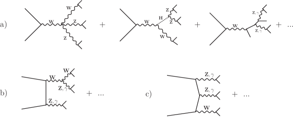
The tree-level diagrams can be grouped into three distinct topologies:
-
a)
The first one (see Fig. 1a) contains all diagrams where there is only one vector boson attached to the quark line, decaying further into 6 leptons.
-
b)
The second topology (see Fig. 1b) comprises all diagrams where exactly two vector bosons are attached to the quark line and then decay into two and four leptons, respectively.
-
c)
The third one (see Fig. 1c) consists of all diagrams where all the three vector bosons are attached to the quark line.
These topologies give rise to different one-loop contributions as will be discussed later.
The parts of the Feynman diagrams that describe the vector bosons decaying into leptons can be seen as effective polarization vectors, computed only once and used for different quark flavor flow. For example, for production, the two different subprocesses and (with an anti-quark, , having the same momentum as the up-quark in the first case, and identical and momenta) share the same effective polarization vectors. These effective polarization vectors are computed numerically at the beginning of the evaluation of the full matrix elements, at a given phase space point, and reused wherever they appear. This reduces the amount of time spent in the calculation of the tree-level matrix elements significantly.
In the calculation of leptonic tensors, special care has to be taken in the treatment of finite-width effects in massive vector boson propagators. In our code, we use the modified complex-mass scheme as implemented in MadGraph, that is we globally replace with , while keeping a real value for [14].
When intermediate Higgs boson exchange effects are included, particular care is needed in the generation of the phase space, since, for small Higgs boson masses (100–300 GeV), the Higgs boson width is very narrow. A Breit-Wigner mapping is needed for the efficient generation of this resonance. In the case of production there are two distinct pairs which can be produced from Higgs boson decay while the Higgs resonance appears only once in and production. For production we, therefore, have generated the boson phase space using Dalitz plot variables which allow for simultaneous Breit-Wigner mappings of two different invariant di-boson masses and thus the two different Higgs resonances. This procedure is very important for good Monte Carlo statistics since the Higgs boson contributions can enhance the LO production cross section by up to a factor of 5 and the NLO production cross section by almost a factor of 4 as shown in Table 1.
| Higgs boson mass [GeV] | [fb] | [fb] |
|---|---|---|
| 60 | ||
| 120 | ||
| 160 | ||
| 180 |
2.2 Real-emission contributions
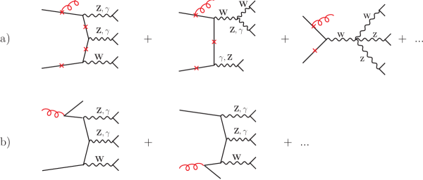
The total NLO cross section is given by the sum of the real emission contributions, the virtual contributions and a collinear term, a finite remnant after the initial-state collinear singularities are absorbed into the parton distribution functions (pdfs). The real emission and virtual contributions are separately infrared divergent in dimensions. In order to deal with these divergences, dimensional reduction () has been used and we apply the dipole subtraction scheme in the formalism proposed by Catani and Seymour [9]. Exact expressions for the dipoles as well as for the finite collinear remnants have already been presented in Ref. [3]. The real-emission matrix elements can be divided into two different classes:
-
a)
Diagrams where the emitted particle is a final-state gluon (see Fig. 2a, where the crosses represent possible gluon-vertex insertions)
-
b)
Diagrams where the emitted particle is a final-state quark, and a gluon is present in the initial state (see Fig. 2b). These diagrams can be obtained by a simple crossing of the diagrams of the previous class. As will be shown in Sec. 3, these diagrams show a stronger scale dependence and are responsible for large -factors in many distributions.
The pre-calculation of the leptonic tensors, as effective polarization vectors, already applied for the LO matrix elements, leads here to an even larger increase in the evaluation speed.
2.3 Virtual contributions
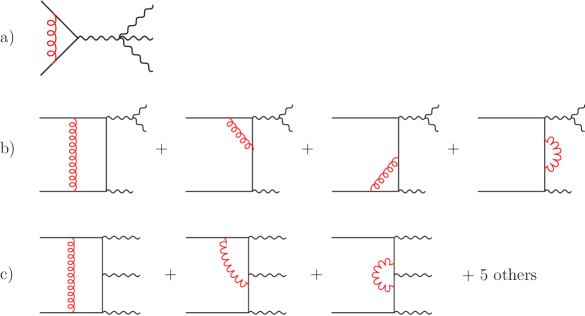
One-loop corrections to the tree-level diagrams of Fig. 1 can be organized according to the three topologies encountered at tree-level:
- a)
- b)
- c)
Since there are only three colored partons in the real-emission diagrams, all infrared singularities appearing in the virtual contribution factorize on the Born amplitude. In conventional dimensional regularization the virtual amplitude is then given by 111 Using dimensional reduction instead, one needs to replace by , but this difference is exactly compensated by an analogous replacement in , the integral of the real-emission counter-term.
| (2.5) |
where is the Born amplitude, the square of the partonic center-of-mass energy and is the finite contribution from the sum of all the one-loop diagrams.
The boxline and pentline contributions have essentially the same analytic expressions found in the calculation of QCD NLO corrections in vector boson fusion processes, and , discussed in Refs. [10] and [11] respectively, apart from crossing a final-state quark to the initial state, and performing then an analytic continuation.
To deal with the finite boxline contribution, we have used the results obtained by a slightly modified version of the boxline routine discussed in Ref. [10]. This routine implements the Passarino-Veltman tensor reduction [12] and leads to quite stable results.
The pentline reduction needs a more stable reduction procedure. We have implemented the method proposed by Denner and Dittmaier [13]. In addition, we have implemented a new calculation of the pentline contributions which reuses intermediate results for different vector boson polarizations. We have checked these results with the pentline routines computed in Ref. [11], after crossing and analytic continuation. The new pentline subroutines turn out to be 4.5 times faster and numerically more stable than the old code. For non-exceptional phase-space points, we found agreement for the two different codes at the 10-8 level. However, even with the increase in speed, this part of the code is still quite slow. Therefore, we have applied a trick, already used in Ref. [2], to reduce the contribution of the pentagon diagrams: we have split the effective polarization vector of a vector boson of momentum into a term proportional to the momentum itself and a remainder
| (2.6) |
The contraction of the pentline contribution with the component aligned along reduces the pentline itself to the difference of boxline contributions. Therefore it is possible to shift part of the pentline contribution to the less time-consuming boxline contributions and calculate the remaining smaller pentline contribution (the one obtained with the contraction with ) with less statistics, without changing the overall Monte Carlo statistical error of the total NLO result [11]. In practice we have chosen
| (2.7) |
for production and
| (2.8) |
for the case.
2.4 Checks
For all the triple boson production processes, we have performed numerous checks on the final results. All matrix elements in the LO and in the real-emission calculation have been checked individually against MadGraph and agree at the 10-15 level. In addition, we have compared the LO cross sections against MadEvent [14] and HELAC [15] and find agreement within the statistical accuracy of the Monte Carlo runs (0.5% for HELAC and 1% for MadEvent). Furthermore, we have implemented Ward identity tests for the virtual contributions and checked the cancellation of divergences in the real emission against their counter-terms, as given by Catani and Seymour [9].
As a final and very important test, we have made a comparison with the already published results for the production of on-shell gauge bosons without leptonic decays of Ref. [3]. Since the authors of this paper have not included Higgs boson exchange and leptonic spin correlations in their calculation, we have neglected these contribution too, i.e. we have neglected the Feynman graphs with Higgs boson exchange and non-resonant contributions and we have used the narrow-width approximation for vector boson decay.
| Scale | program | [fb] | [fb] |
|---|---|---|---|
| VBFNLO | |||
| Ref. [3] | |||
| VBFNLO | |||
| Ref. [3] | |||
| VBFNLO | |||
| Ref. [3] | |||
| VBFNLO | |||
| Ref. [3] |
| Scale | program | [fb] | [fb] |
|---|---|---|---|
| VBFNLO | |||
| Ref. [3] | |||
| VBFNLO | |||
| Ref. [3] | |||
| VBFNLO | |||
| Ref. [3] | |||
| VBFNLO | |||
| Ref. [3] |
In Tables 2 and 3, we show the comparison between the two sets of results, for different factorization- and renormalization-scale choices, here taken to be equal. Our NLO results agree at the 1% level, which is satisfactory, given the same level of agreement for the LO cross sections and the size of the Monte Carlo errors.
3 Results
The calculations described in the previous section have been implemented in a fully flexible parton-level Monte Carlo program, VBFNLO, which originally was developed for the prediction of NLO QCD corrections to vector boson fusion processes. The various triple vector boson production options will be made publicly available soon [7]. The program allows for the calculation of cross sections and distributions in either , or collisions of arbitrary center of mass energy. In the following, we present results on and production at the LHC, i.e. for collisions at TeV.
The default electroweak parameters used in all plots are
| (3.1) |
Two other variables, and , are calculated in the program using LO electroweak relations. We have used the CTEQ6M parton distribution with at NLO and CTEQ6L1 for the LO calculation [16]. All fermions are treated as massless and we do not consider contributions involving bottom and top quarks. The CKM matrix is approximated by a unit matrix throughout. The W- and Z-boson widths have been calculated in the program via tree-level formulas with one loop QCD corrections for the hadronic widths. For Higgs boson decays, approximate formulas are used which incorporate running bottom-quark mass effects and off-shell effects in Higgs decays to weak bosons. For GeV, the resulting widths are
| (3.2) |
In our calculations, the full leptonic final state is available and hence we determine cross sections for realistic acceptance cuts on the leptons. For production, only a cut on the transverse momentum and the rapidity of the final-state charged leptons has been applied. For production we require, in addition, that the invariant mass of any combination of two charged leptons, , to be larger than 15 GeV, in order to avoid virtual-photon singularities in at low . Specifically, we require
| (3.3) |
All results given below have been calculated for three different lepton families in the final state, i.e. interference terms due to identical particles have been neglected. Phenomenologically more interesting are the cases of final states with electrons and/or muons. Considering decays of the three vector bosons into two generations of leptons each, the results for three distinct generations need to be multiplied by a combinatorial factor of four. This takes into account the presence of two identical vector bosons ( and , respectively) and the corresponding symmetry factor of which would appear when considering on-shell weak boson production. These factors are included in all figures.
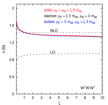
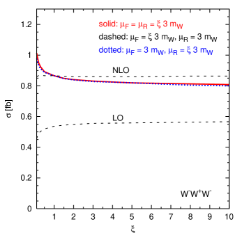
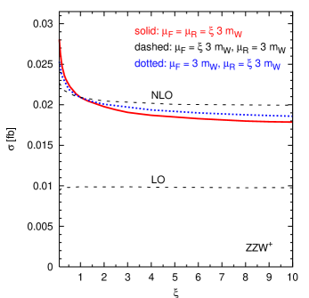
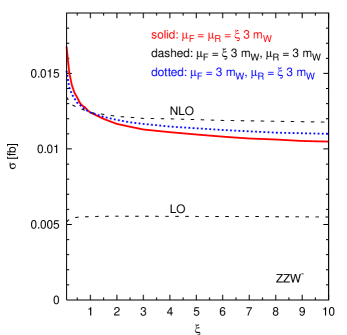
In Figs. 4 and 5, the factorization- () and renormalization-scale () dependence of the LO and the total NLO cross section is shown for all the different processes under investigation. At LO, there is no renormalization-scale dependence, since triple vector boson production is a purely electroweak process. Therefore, the scale variation is only due to the variation of the factorization scale in the parton distribution functions. The small variation at LO can thus be explained by the fact that the pdfs are determined in a Feynman- range of small factorization scale dependence. At NLO, the dependence on the scales is more complicated. Since the factorization-scale dependence is quite small, the dependence under variation of is almost completely dominated by the dependence on the renormalization scale and shows the expected dependence, i.e. the bigger the reference scale, the smaller the scale dependence.
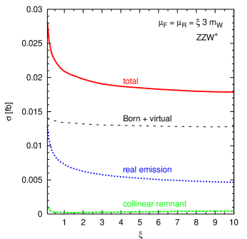
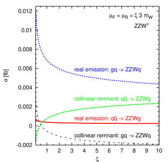
For a more detailed analysis, the different contributions to the total NLO cross section are shown in Fig. 6, for the example of production. A qualitatively similar behavior is found for all triple vector boson processes investigated here. In the left panel of Fig. 6, the finite part of the virtual contributions (the term in Eq. (2.5)), combined with the Born squared terms (including the LO contribution), show a remarkably small dependence under simultaneous variation of the renormalization and the factorization scale. This can be understood by a comparison with the factorization-scale induced LO variation given in Fig. 4. Under variation of , the virtual contribution shows the same behavior as the LO cross section, which means that the cross section decreases for small scales. Under variation of , on the other hand, the finite part of the virtual contribution increases for small scales, due to the increase in . These two opposing behaviors cancel to some extent and lead to the observed curve in Fig. 6.
For the subtracted real-emission contributions and the finite collinear remnants, the analysis of the scale dependence is somewhat more involved, since the finite collinear remnants depend non-trivially both on the factorization and on the renormalization scale. Moreover, these contributions include gluon-induced subprocesses like in addition to the quark-induced ones such as . In the right panel of Fig. 6, the real-emission contributions and the finite collinear remnants are therefore separately shown for each of these classes of subprocesses.
In the finite collinear remnants, the quark- and gluon-induced contributions show opposite behavior under variation of the scale. Due to these cancellations, the resulting scale dependence and the size of their overall contribution is very small. The real-emission contributions arising from the quark-induced subprocesses show a similar scale dependence and are almost constant for the scales shown here. A comparatively large scale variation is observed in the real-emission terms of the gluon-induced contributions. These are also responsible for the large scale dependence of the overall real-emission term in the left panel of Fig. 6. This is not surprising since gluon-initiated subprocesses open up for the first time at NLO, and therefore, a LO-type scale dependence is expected. Gluon-induced subprocesses are also responsible for a large fraction of the -factor. For instance, the -factor for production at is 2.1, whereas the -factor without gluon-initiated subprocesses only amounts to 1.5.
In our analysis, we have also checked other scale choices, such as the invariant 3-vector boson mass or the minimal of the three vector bosons. We could not find an improved scale dependence, however, either in the cross section or in the distributions. This again can be understood since the dominating scale dependence comes from the gluon-induced subprocesses, which have to be considered as LO processes.
For all processes studied, we have found a strong phase-space dependence of the size of NLO corrections. Thus, differential -factors, defined as the ratio of NLO over LO differential distributions,
| (3.4) |
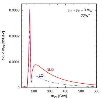
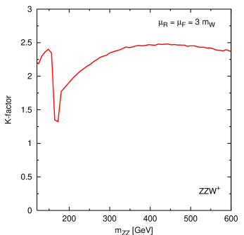
can show a considerable variation. In the left panel of Fig. 7, for instance, the invariant mass distribution in production is shown for a Higgs boson mass of GeV. Here the Higgs boson contribution gives rise to the narrow peak at about GeV. At tree level, the only Feynman graph with a Higgs boson exchange is the one depicted in Fig. 1a, where the Higgs boson decays into two Z bosons. This graph dominates near . In the right panel, we have plotted the differential -factor. Since the QCD corrections to the Higgs boson-contribution itself increase the cross section only by about 30% [17], there is a pronounced dip in the differential -factor at about the Higgs boson mass.
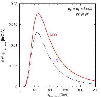
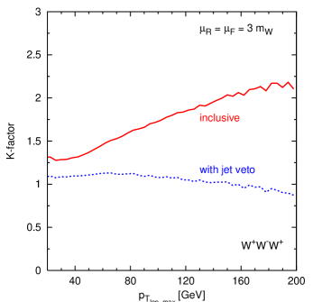
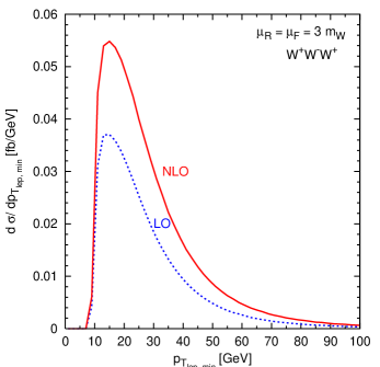
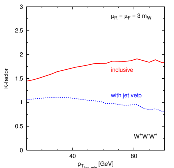
In Figs. 8 and 9, we give two more examples of the phase-space dependence of the NLO corrections for production at GeV. In Fig. 8, the transverse-momentum distribution and the -factor of the highest- charged lepton are shown while Fig. 9 shows the same for the charged lepton of lowest-. Variation of the -factor up to 70% is observed for the highest- lepton while for the lowest- lepton we have variations up to 30% when considering “inclusive” event samples. This -dependence of the -factors can be traced to the kinematics of the real-emission contributions. The rise is mostly due to events with high jets which are recoiling against the leptons. Imposing a veto on jets with GeV leads to a fairly flat -factor which, in addition, is close to unity for the lepton distributions (curves labeled “with jet veto” in Figs. 8 and 9). Similar effects had previously been observed for vector boson pair production at the LHC [5].
4 Conclusions
The simulation of triple vector boson production at the LHC is important for two reasons. These processes are a Standard Model background for new-physics searches which are characterized by multi-lepton final states, and secondly they are sensitive to quartic electroweak couplings. In this paper, we have presented first results for the full NLO differential cross sections for and production, with all spin correlations from leptonic vector boson decays, intermediate Higgs boson-exchange effects and off-shell contributions taken into account. Results are collected in a fully flexible Monte Carlo program, VBFNLO [7].
When varying the factorization and the renormalization scale up and down by a factor of 2 around the reference scale , we have found a scale dependence of about 5% for the LO cross section and of somewhat less than 10% for the NLO cross section, for production. For the case, the LO scale dependence is around 1%, whereas the dependence of the NLO cross section is around 13%. These variations are in the expected range for the NLO scale dependence, while the LO variations have to be considered anomalously small, due to the absence of initial-state gluon-induced subprocesses. The large -factors (of order 2 and even larger in some phase-space regions) demonstrate the importance of including the NLO QCD corrections on top of the LO predictions.
The differential -factors for several distributions for both of these processes are highly dependent on the Higgs boson mass. In general we observe that the larger the contributions from the Higgs boson are, the smaller is the -factor. In the case of the production, with , for example, the -factor decreases from 1.6 for a Higgs boson mass of 120 GeV to 1.4 for a Higgs boson mass of 150 GeV. At the same time the LO cross section increases by more than a factor of 2. Therefore, in all simulations, the Higgs boson contribution has to be taken into account in order to obtain a valid prediction for the cross sections and the -factors. Besides these large -factors, we have also found a strong phase-space dependence of the size of the NLO corrections which shows that a mere multiplication of distributions by an overall -factor is not sufficient.
Acknowledgments
We would like to thank Malgorzata Worek for the comparison with HELAC and Thomas Binoth and Giovanni Ossola and collaborators for the comparison with their results. C.O. and D.Z. would like to thank the KITP at UC Santa Barbara for its hospitality during part of our work. This research was supported in part by the Deutsche Forschungsgemeinschaft via the Sonderforschungsbereich/Transregio SFB/TR-9 “Computational Particle Physics” and the Graduiertenkolleg “High Energy Physics and Particle Astrophysics” and in part by the National Science Foundation under Grant No. PHY05-51164. F.C. acknowledges a postdoctoral fellowship of the Generalitat Valenciana (Beca Postdoctoral d‘Excelléncia). The Feynman diagrams in this paper were drawn using Jaxodraw [18].
References
- [1] A. Lazopoulos, K. Melnikov and F. Petriello, Phys. Rev. D 76 (2007) 014001 [arXiv:hep-ph/0703273].
- [2] V. Hankele and D. Zeppenfeld, Phys. Lett. B 661 (2008) 103 [arXiv:0712.3544 [hep-ph]].
- [3] T. Binoth, G. Ossola, C. G. Papadopoulos and R. Pittau, JHEP 0806 (2008) 082 [arXiv:0804.0350 [hep-ph]].
- [4] See for example J. Ohnemus, Phys. Rev. D 44 (1991) 1403; L. J. Dixon, Z. Kunszt and A. Signer, Nucl. Phys. B 531 (1998) 3 [arXiv:hep-ph/9803250]; L. J. Dixon, Z. Kunszt and A. Signer, Phys. Rev. D 60 (1999) 114037 [arXiv:hep-ph/9907305].
- [5] J. Ohnemus, Phys. Rev. D 44 (1991) 3477; J. Ohnemus, Phys. Rev. D 50 (1994) 1931 [arXiv:hep-ph/9403331]; U. Baur, T. Han and J. Ohnemus, Phys. Rev. D 51 (1995) 3381 [arXiv:hep-ph/9410266]; U. Baur, T. Han and J. Ohnemus, Phys. Rev. D 53 (1996) 1098 [arXiv:hep-ph/9507336].
- [6] J. M. Campbell and R. K. Ellis, Phys. Rev. D 60 (1999) 113006 [arXiv:hep-ph/9905386].
-
[7]
The VBFNLO code is available at
http://www-itp.particle.uni-karlsruhe.de/~vbfnloweb/ - [8] K. Hagiwara and D. Zeppenfeld, Nucl. Phys. B 274 (1986) 1; K. Hagiwara and D. Zeppenfeld, Nucl. Phys. B 313 (1989) 560.
- [9] S. Catani and M. H. Seymour, Nucl. Phys. B 485 (1997) 291 [Erratum-ibid. B 510 (1998) 503] [arXiv:hep-ph/9605323].
- [10] C. Oleari and D. Zeppenfeld, Phys. Rev. D 69 (2004) 093004 [arXiv:hep-ph/0310156].
- [11] B. Jager, C. Oleari and D. Zeppenfeld, JHEP 0607 (2006) 015 [arXiv:hep-ph/0603177]; G. Bozzi, B. Jager, C. Oleari and D. Zeppenfeld, Phys. Rev. D 75 (2007) 073004 [arXiv:hep-ph/0701105].
- [12] G. Passarino and M. J. G. Veltman, Nucl. Phys. B 160 (1979) 151.
- [13] A. Denner and S. Dittmaier, Nucl. Phys. B 658, 175 (2003) [arXiv:hep-ph/0212259]; A. Denner and S. Dittmaier, Nucl. Phys. B 734, 62 (2006) [arXiv:hep-ph/0509141].
- [14] T. Stelzer and W. F. Long, Comput. Phys. Commun. 81 (1994) 357 [arXiv:hep-ph/9401258]; F. Maltoni and T. Stelzer, JHEP 0302 (2003) 027 [arXiv:hep-ph/0208156].
- [15] A. Cafarella, C. G. Papadopoulos and M. Worek, arXiv:0710.2427 [hep-ph]; C. G. Papadopoulos and M. Worek, Eur. Phys. J. C 50 (2007) 843 [arXiv:hep-ph/0512150]. A. Kanaki and C. G. Papadopoulos, Comput. Phys. Commun. 132 (2000) 306 [arXiv:hep-ph/0002082].
- [16] J. Pumplin, D. R. Stump, J. Huston, H. L. Lai, P. Nadolsky and W. K. Tung, JHEP 0207 (2002) 012 [arXiv:hep-ph/0201195].
- [17] T. Han and S. Willenbrock, Phys. Lett. B 273 (1991) 167; J. Ohnemus and W. J. Stirling, Phys. Rev. D 47 (1993) 2722; H. Baer, B. Bailey and J. F. Owens, Phys. Rev. D 47 (1993) 2730; M. Spira, Fortsch. Phys. 46 (1998) 203 [arXiv:hep-ph/9705337]; O. Brein, M. Ciccolini, S. Dittmaier, A. Djouadi, R. Harlander and M. Kramer, arXiv:hep-ph/0402003.
- [18] D. Binosi and L. Theussl, Comput. Phys. Commun. 161, 76 (2004) [arXiv:hep-ph/0309015].