On measuring the gravitational-wave background using Pulsar Timing Arrays
Abstract
Long-term precise timing of Galactic millisecond pulsars holds great promise for measuring the long-period (months-to-years) astrophysical gravitational waves. Several gravitational-wave observational programs, called Pulsar Timing Arrays (PTA), are being pursued around the world.
Here we develop a Bayesian algorithm for measuring the stochastic gravitational-wave background (GWB) from the PTA data. Our algorithm has several strengths: (1) It analyses the data without any loss of information, (2) It trivially removes systematic errors of known functional form, including quadratic pulsar spin-down, annual modulations and jumps due to a change of equipment, (3) It measures simultaneously both the amplitude and the slope of the GWB spectrum, (4) It can deal with unevenly sampled data and coloured pulsar noise spectra. We sample the likelihood function using Markov Chain Monte Carlo (MCMC) simulations. We extensively test our approach on mock PTA datasets, and find that the algorithm has significant benefits over currently proposed counterparts. We show the importance of characterising all red noise components in pulsar timing noise by demonstrating that the presence of a red component would significantly hinder a detection of the GWB
Lastly, we explore the dependence of the signal-to-noise ratio on the duration of the experiment, number of monitored pulsars, and the magnitude of the pulsar timing noise. These parameter studies will help formulate observing strategies for the PTA experiments.
keywords:
gravitational waves – methods: data analysis – pulsars: general1 Introduction
At the time of this writing several large projects are being pursued in order to directly detect astrophysical gravitational waves. This paper concerns a program to detect gravitational waves using pulsars as nearly-perfect Einstein clocks. The practical idea is to time a set of millisecond pulsars (called the “Pulsar Timing Array”, or PTA) over a number of years (Foster & Backer, 1990). Some of the millisecond pulsars create pulse trains of exceptional regularity. By perturbing the space-time between a pulsar and the Earth, the gravitational waves (GWs) will cause extra deviations from the periodicity in the pulse arrival times (Estabrook & Wahlquist, 1975; Sazhin, 1978; Detweiler, 1979). Thus from the measurements of these deviations (called “timing-residuals”, or TR), one may measure the gravitational waves. Currently, several PTA project are operating around the globe. Firstly, at the Arecibo Radio Telescope in North-America several millisecond pulsars have been timed for a number of years. These observations have already been used to place interesting upper limits on the intensity of gravitational waves which are passing through the Galaxy (Kaspi et al., 1994; Lommen, 2001). Together with the Green Bank Telescope, the Arecibo Radio Telescope will be used as an instrument of NANOGrav, the North American PTA. Secondly, the European PTA is being set up as an international collaboration between Great Britain, France, Netherlands, Germany, and Italy, and will use 5 European radio telescopes to monitor about 20 millisecond pulsars (Stappers et al., 2006). Finally, the Parkes PTA in Australia has been using the Parkes multi-beam radio-telescope to monitor 20 millisecond pulsars (Manchester, 2006). Some of the Parkes and Arecibo data have also been used to place the most stringent limits on the GWB to date (Jenet et al., 2006).
One of the main astrophysical targets of the PTAs is the stochastic background of the gravitational waves (GWB). This GWB is thought to be generated by a large number of black-hole binaries which are thought to be located at the centres of galaxies (Begelman et al., 1980; Phinney, 2001; Jaffe & Backer, 2003; Wyithe & Loeb, 2003; Sesana et al., 2005), by relic gravitational waves (Grishchuk, 2005), or, more speculatively, by cusps in the cosmic-string loops (Damour & Vilenkin, 2005). This paper develops an algorithm for the optimal PTA measurement of such a GWB.
The main difficulty of such a measurement is that not only Gravitational
Waves create the pulsar timing-residuals. Irregularities of the pulsar-beam
rotation (called the “timing noise”), the receiver noise, the imprecision
of local clocks, the polarisation calibration of the telescope
(Britton, 2000), and the variation in the refractive index of the
interstellar medium all contribute significantly to the timing-residuals,
making it a challenge to separate these noise sources from the
gravitational-wave signal. However, the GWB is expected to induce
correlations between the timing-residuals of different pulsars. These
correlations are of a specific functional form [given by
Eq. (9) below], which is different from those introduced by
other noise sources (Hellings &
Downs, 1983). Jenet
et al. (2005, hereafter J05)
have invented a clever algorithm which uses the uniqueness of the
GWB-induced correlations to separate the GWB from other noise sources, and
thus to measure the magnitude of the GWB. Their idea was to measure the
timing-residual correlations for all pairs of the PTA pulsars, and check how
these correlations depend on the sky-angles between the pulsar pairs. J05
have derived a statistic which is sensitive to the functional form of the
GWB-induced correlation; by measuring the value of this statistic one can
infer the strength of the GWB. While J05 algorithm appears robust, we
believe that in its current form it does have some drawbacks, in particular:
(1) The statistic used by J05 is non-linear and non-quadratic in the
pulsar-timing-residuals, which makes its statistical properties
non-transparent.
(2) The pulsar pairs with the high and low intrinsic timing noise make
equal contributions to the J05 statistic, which is clearly not
optimal.
(3) The J05 statistic assumes that the timing-residuals of all the PTA
pulsars are measured during each observing run, which is generally not the
case.
(4) The J05 signal-to-noise analysis relies on the prior knowledge of the
intrinsic timing noise, and there is no clean way to separate this timing
noise from the GWB.
(5) The prior spectral information on GWB is used for whitening the signal;
however, there is no proof that this is an optimal procedure. The spectral
slope of the GWB is not measured.
In this paper we develop an algorithm which addresses all of the problems outlined above. Our method is based on essentially the same idea as that of J05: we use the unique character of the GWB-induced correlations to measure the intensity of the GWB. The algorithm we develop below is Bayesian, and by construction uses optimally all of the available information. Moreover, it deals correctly and efficiently with all systematic contributions to the timing-residuals which have a known functional form, i.e. the quadratic pulsar spin-downs, annual variations, one-time discontinuities (jumps) due to equipment change, etc. Many parameters of the timing model (the model popular pulsar timing packages use to generate TRs from pulsar arrival times) fall in this category.
The plan of the paper is as follows. In the next section we review the theory of the GWB-generated timing residuals and introduce our model for other contributions to the timing residuals. In Sec. 3 we explain the principle of Bayesian analysis for GWB-measurement with a PTA, and we evaluate the Bayesian likelihood function. There we also show how to analytically marginalise over the contributions of known functional form but unknown amplitude (i.e., annual variations, quadratic residuals due to pulsar spin-down, etc.). The details of this calculation are laid out in Appendix A. Section 4 discusses the numerical integration technique which we use in our likelihood analysis: the Markov Chain Monte Carlo (MCMC). In Sec. 5 we show the analyses of mock PTA datasets. For each mock dataset, we construct the probability distribution for the intensity of the GWB, and demonstrate its consistency with the input mock data parameters. We study the sensitivity of our algorithm for different PTA configurations, and investigate the dependence of the signal-to-noise ratio on the duration of the experiment, on redness and magnitude of the pulsar timing noise, and on the number of clocked pulsars. In Sec. 6 we summarise our results.
2 The Theory of GW-generated timing-residuals
2.1 Timing residual correlation
The measured millisecond-pulsar timing-residuals contain contributions from several stochastic and deterministic processes. The latter include the gradual deceleration of the pulsar spin, resulting in a pulsar rotational period derivative which induces timing residuals varying quadratically with time (hereafter referred to as “quadratic spin-down”), the annual variations due to the imperfect knowledge of the pulsar positions on the sky, the ephemeris variations caused by the known planets in the solar system, and the jumps due to equipment change (Manchester 2006). The stochastic component of the timing-residuals will be caused by the receiver noise, clock noise, intrinsic timing noise, the refractive index fluctuations in the interstellar medium, and, most importantly for us, the GWB. For the purposes of this paper we restrict ourselves to considering the quadratic spin-downs, intrinsic timing noise, and the GWB; other components can be similarly included, but we omit them for mathematical simplicity. In this case, the timing residual of the pulsar can be written as
| (1) |
where and are caused by the GWB and the pulsar timing noise, respectively, and
| (2) |
represent the quadratic spin-down. One expects the timing noise from different pulsars to be uncorrelated, while the GWB will cause correlations in the timing-residuals between different pulsars. Therefore, the information about GWB can be extracted by correlating the timing residual data between the different pulsars (J05). If one assumes that both GWB-generated residuals and the intrinsic timing noise are stochastic Gaussian processes, then we can represent them by the coherence matrices:
| (3) |
with the total coherence matrix given by
| (4) |
The timing-residuals are then distributed as a multidimensional Gaussian:
| (5) | |||||
where denotes the probability distribution of the timing-residuals.
To be able to use Eq. (5) we must
(1) be able to evaluate the GWB-induced coherence matrix from
the theory, as a function of variables that parametrise the GWB spectrum,
and
(2) introduce well-motivated parametrization of the pulsar timing noise.
In this work, the spectral density of the stochastic GW
background is taken to be a power law (Phinney, 2001; Jaffe &
Backer, 2003; Wyithe & Loeb, 2003; Maggiore, 2000)
| (6) |
where represents the spectral density, is the GW amplitude, is the GW frequency, and is an exponent characterising the GWB spectrum. If the GWB is dominated by the supermassive black hole binaries, then (Phinney 2001). This definition is equivalent to the use of the characteristic strain as defined in Jenet et al. (2006):
| (7) |
with . The GWB-induced coherence matrix is then given by
| (8) | |||||
Here is the geometric factor given by
| (9) |
where is the angle between pulsar and pulsar (Hellings & Downs, 1983), , is the gamma function, and is the low cut-off frequency, chosen so that is much greater than the duration of the PTA operation. Introducing is a mathematical necessity, since otherwise the GWB-induced correlation function would diverge. However, we show below that the low-frequency part of the GWB is indistinguishable from an extra spin-down of all pulsars which we already correct for, and that our results do not depend on the choice of provided that .
The pulsar timing noise is assumed to be Gaussian, with a certain functional form of the power spectrum. The true profile of the millisecond pulsar timing noise spectrum is not well-known at present time. The timing residuals of the most precisely observed pulsars indicate that pulsar timing noise has a white and poorly-constrained red component (J. Verbiest and G. Hobbs, private communications).
For the purposes of this paper we will always choose the spectra to be
of the same functional form for all pulsars, but this is not an inherent limitation of the
algorithm. We consider 3 cases of pulsar timing noise
spectra:
(1) White (flat) spectra
(2) Lorentzian spectra
(3) Power-law spectra
Obviously, one could also consider a timing noise which is a superposition of these components;
we do not do this at this exploratory stage.
If we choose the pulsar timing noise spectrum to be white, with an
amplitude , the resulting correlation matrix becomes:
| (10) |
The Lorentzian spectrum is a red spectrum with a typical frequency that determines the redness of the timing noise:
| (11) |
which yields the following correlation matrix:
| (12) |
where is a typical frequency and is the amplitude.
By using a power law spectral density with amplitude and spectral index , one gets a timing-noise coherence matrix analogous to the one in Eq. (8):
| (13) | |||||
3 Bayesian approach
3.1 Basic ideas
The method described in this report is based upon a Bayesian approach to
the parameter inference. The general idea of the method is to (a) assume
that the physical processes which produce the timing-residuals can be
characterised by several parameters, and (b) use the Bayes theorem to
derive from the measured data the probability distribution of the
parameters of our interest. In our case, we assume that the timing
residuals are created by
(1) the GWB; we parametrise it by its amplitude and slope , as
in equation (6).
(2) the intrinsic timing noise of the 20 monitored millisecond pulsars. We
assume that the timing noise of each of the pulsars is the random Gaussian
noise, with a variety of possible spectra described in the previous
section. We shall refer to the variables parametrizing the timing noise
spectral shape as .
(3). The quadratic spin-downs, parametrised for each of the pulsars by
, , and , cf. Eq. (2).
With these assumptions, we shall write down below the expression for the probability distribution of the data, as a function of the parameters. By Bayes theorem, we can then compute the posterior distribution function; the probability distribution of the parameters given a certain dataset:
Here is the prior probability of the unknown parameters, which represents all our current knowledge about these parameters, and is the Bayesian evidence, which we will use here as a normalisation factor to ensure that integrates to unity over the parameter space. We note here that the Bayesian evidence is in essence a goodness of fit measure that can be used for model selection. However, we will ignore the Bayesian evidence in this work and postpone the model selection part of the algorithm to future work. For our purposes, we are only interested in and , which means that we have to integrate over all of the other parameters. Luckily, as we show below, for a uniform prior the integration over , , and can be performed analytically. This amounts to the removal of the quadratic spin-down component to the pulsar data. We emphasise that this removal technique is quite general, and can be readily applied to unwanted signal of any known functional form (i.e., annual modulations, jumps, etc.—see Sec. 3.2), even if those parameters have already been fit for while calculating the timing residuals. The integration over must be performed numerically.
In this work we shall use MCMC simulation as a multi dimensional integration technique. Besides flat priors for most of the parameters, we will use slightly peaked priors for parameters which have non-normalisable likelihood functions. This ensures that the Markov Chain can converge.
In the rest of the paper, we detail the implementation and tests of our algorithm.
3.2 Removal of the quadratic spin-downs and other systematic signals of known functional form
While this subsection is written with the PTA in mind, it may well be useful for other applications in pulsar astronomy. We thus begin with a fairly general discussion, and then make it more specific for the PTA case.
Consider a random Gaussian process with a coherence matrix , which is contaminated by several systematic signals with known functional forms but a-priori unknown amplitudes . Here is a set of interesting parameters which we want to determine from the data . The resulting signal is given by
| (15) |
or, in the vector form, by
| (16) |
Here the components of the vectors , , and are given by , , and , respectively, and is the non-square matrix with the elements . Note that the dimensions of and are different. The Bayesian probability distribution for the parameters is given by
| (17) | |||||
where is the prior probability and is the normalisation. Since we are only interested in , we can integrate over the variables . This process is referred to as marginalisation; it can be done analytically if we assume a flat prior for [i.e., if is -independent], since enter at most quadratically into the exponential above. After some straightforward mathematics which we have detailed in Appendix A, we get
where is the normalisation, and
| (19) |
and the -superscript stands for the transposed matrix. Equation (3.2) is one of the main equations of the paper, since it provides a statistically rigorous way to remove (i.e., marginalise over) the unwanted systematic signals from random Gaussian processes. One can check directly that the above expression for is insensitive to the values of the amplitudes of the systematic signals in the Eq. (15).
We now apply this formalism to account for the quadratic spin-downs in the PTA. As in Sec. 2, it will be convenient to use the 2-index notation for the timing-residuals, measured at the time , where is the pulsar index, and is the number of the timing residual measurement for pulsar . The space of the spin-down parameters , has dimensions, where is the number of pulsars in the array. In the component language, we write
| (20) |
where
| (21) |
is the part of the timing residual due to a random Gaussian process (i.e., GWB, timing noise, etc.), and . The quantities are components of the matrix operator which acts on the -dimensional vector in the parameter space and produces a vector in the timing-residual space. For example, for 20 pulsars, each with 250 timing residual observations, the matrix has rows, each marked by 2 indices , , and columns, each marked by 2 indices , . Thus in the vector form, one can write Eq. (20) as
| (22) |
which is identical to the Eq. (16). We thus can use Eq. (3.2) to remove the quadratic spin-down contribution from the PTA data.
Although we only demonstrate this technique for quadratic spin-down, this
removal technique will be useful for treating other noise sources in the
PTA. All sources of which the functional form is known (and therefore can
be fit for, as most popular pulsar timing packages do) can be dealt with,
i.e.
(1) Annual variation of the timing-residuals due to the imprecise
knowledge of the pulsar position on the sky. The annual variation in each
of the pulsars will be a predictable function of the associated 2 small
angular errors (latitude and longitude). Thus our parameter space will
expand by 2N, but this will still keep the matrix manageable.
(2) Changes of equipment will introduce extra jumps, and must be taken
into account. This is trivial to deal with using the techniques described
above.
(3) Some of the millisecond pulsars are in binaries, and their orbital
motion must be subtracted. The errors one makes in these subtractions will
affect the timing-residuals. They can be parametrised and dealt with using
the techniques of this section (we thank Jason Hessels for pointing this
out).
3.3 Low-frequency cut-off
All predictions for GWB spectrum show a steep power law , where for black-hole binaries (Phinney, 2001). Physically, there is a low-frequency cut-off to the spectrum, due to the fact that black-hole binaries with periods greater than years shrink mostly due to the external friction (i.e., scattering of circum-binary stars or excitation of density waves in a circum-binary gas disc), and not to gravitational radiation. However, while the exact value of the low-frequency cut-off is poorly constrained, the PTA should not be sensitive to it since the duration of the currently planned experiments is much shorter than years. In this subsection, we show this formally by explicitly introducing the low-frequency cut-off and by demonstrating that our Bayesian probabilities are insensitive to its value.
Consider the expression in Eq. (8) for the GWB-generated correlation matrix for the timing-residuals. This expression contains an integral of the form
| (23) |
where . When the low-frequency cut-off is much smaller than the inverse of the experiment duration, i.e. when , the integral above can be expanded as
| (24) |
where
| (25) |
In the expansion above we have assumed . The terms which contain diverge when goes to zero, and scale as or with respect to the time interval. We now show that these divergent terms get absorbed in the process of elimination of the quadratic spin-downs.
Suppose that we add to the timing-residuals of a pulsar a quadratic spin-down term, . The spin-down-removal procedure described in the previous section makes our results completely insensitive to this addition: ’s could be arbitrarily large but the measured GWB would still be the same. Clearly, the same is true if one treats , , not as fixed numbers, but as random variables drawn from some Gaussian distribution. The correlation introduced into the timing-residuals by adding a random quadratic spin-down is given by
The -dependent part of Eq. (24) contains terms which scale as , , and , and thus have the same functional dependence as some of the terms in Eq. (3.3). Since the terms in Eq. (3.3) can be made arbitrarily large, it is clear that the terms corresponding to the low-frequency cutoff could be absorbed into the correlation function corresponding to the quadratic spin-down with the stochastic coefficients. We have made this argument for the timing-residuals from a single pulsar, but it is trivial to extend it to the case of multiple pulsars. Thus our results are not sensitive to the actual choice of the so long as ; this is confirmed by direct numerical tests.
4 Numerical integration techniques
4.1 Metropolis Monte Carlo
The Bayesian probability distribution for the PTA is computed in multi dimensional parameter space, where all of the parameters except 2 characterise intrinsic pulsar timing noise and other potential interferences. To obtain meaningful information about the GWB, we need to integrate the probability function over all of the unwanted parameters. This is a challenging numerical task: a direct numerical integration over more than several parameters is prohibitively computationally expensive. Fortunately, numerical shortcuts do exist, and the most common among them is the Markov Chain Monte Carlo (MCMC) simulation. In a typical MCMC, a set of semi-random walkers sample the parameter space in a clever way, each generating a large number of sequential locations called a chain (Newman & Barkema, 1999). After a sufficient number of steps, the density of points of the chain becomes proportional to the Bayesian probability distribution. The number of steps required for the chain convergence scales linearly with the number of dimensions of the parameter space; typically few steps are required for reliable convergence. In this paper we use the Metropolis (Newman & Barkema, 1999) algorithm for generating the chain, which can be used with an arbitrary distribution, the proposal distribution, for generating new locations of the chain. We use a Gaussian proposal distribution, centred at the current location in the parameter space. During an initial period, the burn-in period, the width of the proposal distribution in all dimensional directions is set to yield the asymptotically optimal acceptance rate of for the Metropolis algorithm (Roberts et al., 1997). At the end of the MCMC simulation we check the convergence of the chain using the bootstrap method (Efron, 1979). We also calculate the global maximum likelihood value for all parameters using a conjugate directions search (Brent, 1973).
4.2 Current MCMC computational cost
The greatest computational challenge in constructing the chain is the fast evaluation of the matrix in Eqs. (3.2)&(19). If timing-residuals are measured for each of the pulsars (50 weeks for 5 years), the size of the matrix becomes . We find it takes about seconds to invert and thus about times as much to arrive to the next point in the chain. Therefore, for the required chain points to get the convergent distribution, we need of order month of the single-processor computational time. On a cluster this can be done in a couple of days. We emphasize that this is an order process. For matrices of the calculation can be done overnight on a single modern workstation, but for the calculation is already a serious challenge.
For the currently projected size of the datasets (Manchester, 2006), the amount of timing-residuals will most likely not exceed the (Hobbs, private communications). Thus, the brute-force method presented here is not computationally expensive for the projected data volume over the next 5 years.
4.3 Choosing a suitable prior distribution
For some models (e.g. the power law spectal density for pulsar timing noise) the likelihood function proves to be not normalisable. This would pose a serious problem in combination with uniform priors as the nuisance parameters then cannot be marginalised and the posterior cannot represent a probability distribution. Although this is a sign that our model is incorrect (infinite Bayesian Evidence/normalisation), this can be easily solved with a different parameterisation. We can always change coordinates in parameter space to a set for which all parameters have a finite domain, which guarantees that our likelihood function is normalisable. This procedure is equivalent to choosing a different prior (the Jacobian in the case of a coordinate transformation) for the original set. We therefore argue that we need to choose an appropriate prior for the non-normalisable parameters. We propose to use a Lorentzian shaped profile:
| (27) |
where is the parameter for which we are construction a prior, and is some typical width/value for this parameter.
As an example we show the likelihood function and the prior for the pulsar timing noise spectral index parameter of Eq. (13) in Fig. 1. The likelihood function seems to drop to zero for high , but it actually has a non-negligible value for all greater than the maximum likelihood value. The broadness of the prior is chosen such that it does not change the representation of the significant part of the likelihood in the posterior, but it does make sure that the posterior is normalisable.

4.4 Generating mock data
In order to generate mock data, we produce a realization of the multi dimensional Gaussian process of Eq. (5), as follows. We rewrite Eq. (5) is a basis in which is diagonal:
| (28) |
where,
| (29) |
Here are the eigenvalues of , and
| (30) |
where is the transformation matrix which diagonalizes :
| (31) |
Thus we follow the following steps:
(1) Diagonalize matrix , find
and .
(2) Choose from random gaussian
distributions of widths .
(3) Compute the timing
residuals via Eq. (30).
It is then trivial to add deterministic processes, like quadratic spin-downs, to the simulated timing-residuals.
5 Tests and parameter studies
We test our algorithm by generating mock timing-residuals for a number of millisecond pulsars which are positioned randomly in the sky. We found it convenient to parametrise the GWB spectrum by [cf.Eq. (6)]
| (32) |
Our mock timing-residuals are a single realisation of GWB for some values of
and and the pulsar timing noise. Random quadratic-spin-down
terms are added. We then perform several separate investigations as
follows:
5.1 Single dataset tests
Our algorithm is tested on several datasets in the following way:
The mock datasets were generated with parameters resembling an experiment
of pulsars, with observations approximately every weeks for
years. The pulsar timing noise was set to an optimistic level of ns
each (rms timing residuals). In all cases the level of GWB has been set to
, with . This level of GWB is an
order of magnitude smaller than the most recent upper limits of this
type(Jenet et al., 2006). We then analyze this mock data using the MCMC
method. In Figs 2—4 we see
examples of the joint — probability distribution, obtained by
these analyses. For each dataset we also calculate the maximum likelihood
value of all parameters using a conjugate directions search. The algorithm
gives results consistent with the input parameters (i.e., they recover the
amplitude and the slope of the GWB within measurement errors). This was
observed in all our tests.
For all datasets we also calculated the Fisher information matrix, a matrix consisting of second-order derivatives to all parameters, at the maximum likelihood points. We can use this matrix to approximate the posterior by a multi dimensional Gaussian, since for some particular models this approximation is quite good. The Fisher information matrix can be calculated in a fraction of the time needed to perform a full MCMC analysis. For all datasets we have plotted the contour of the multi dimensional Gaussian approximation.
As an extra test, we have also used datasets generated by the popular pulsar timing package tempo2 (Hobbs et al., 2006) with a suitable GWB simulation plug-in (Hobbs et al., in preparation). We were able to generate datasets with exactly the same parameters as with our own algorithm, provided that the timing noise was white. We have confirmed that those datasets yield similar results when analysed with our algorithm.


An important point is that that the spectral form of the timing noise has a large impact on the detectability of the GWB. For a red Lorentzian pulsar timing noise there is far greater degeneracy between the spectral slope and amplitude in the timing residual data for the GWB than for white pulsar timing noise, and thus the overall signal-to-noise ratio is significantly reduced by the red component of the timing noise.
5.2 Multiple datasets, same input parameters
To estimate the robustness of our algorithm, we also perform a maximum
likelihood search on many datasets:
(a) We generate a multitude of mock timing-residual data for the same PTA
configurations as in Sec. 5.1, with white timing
noise.
(b) For every one of these datasets we calculate the maximum likelihood
parameters using the conjugate directions search. The ensemble of maximum
likelihood estimators for () should be close to the true values
used to generate the timing-residuals.
The results of maximum likelihood search on many datasets is demonstrated in Fig. 5. The points are the maximum likelihood values for individual datasets. It can be seen that the points are distributed in a shape similar, but not identical, to Fig. 2: some points are quite far off from the input parameters. In order to test the validity of the results, we calculate the Fisher information matrix at the maximum likelihood points, and show the contour of the multidimensional Gaussian approximation based on the Fisher information matrix for three points. We wee that the error contours do not exclude the true values at high confidence, even though the Fisher matrix does not yield a perfect representation of the error contours (the true posterior is not perfectly Gaussian), and we have a posteriori selected outliers for 2 of the 3 cases.

5.3 Parameter studies
To test the accuracy of the algorithm, and to provide suggestions for
optimal PTA configurations, we conduct some parameter studies on
simplified sets of mock timing-residuals:
(a) We generate many sets of mock timing-residuals for the simplified case
of white pulsar timing noise spectra, all with the same white noise
amplitude. The datasets are timing-residuals for some number of millisecond pulsars
which are positioned randomly in the sky. We parametrize the GWB by Eq. (32). We then generate many sets of timing-residuals, varying
several parameters [i.e., timing noise amplitude (assumed the same for all pulsars),
duration of the experiment, and number of pulsars].
(b) For each of the mock datasets we approximate the likelihood function
by a Gaussian in the GWB amplitude , with all other parameters fixed to
their real value. We use as a free parameter since it represents the
strength of the GWB, and therefore the accuracy of is a measure of the
detectability. All other parameters are fixed to keep the computational
time low, but this does result in a higher signal to noise ratio than is
obtainable with a full MCMC analysis.
(c) For this Gaussian approximation, we calculate the ratio
as an estimate for the signal to noise ratio, where
is the value of at which the likelihood function maximizes, and
is the value of the standard deviation of the Gaussian
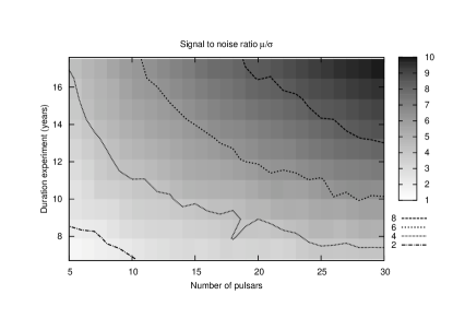
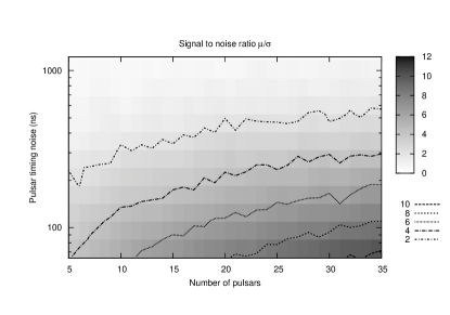
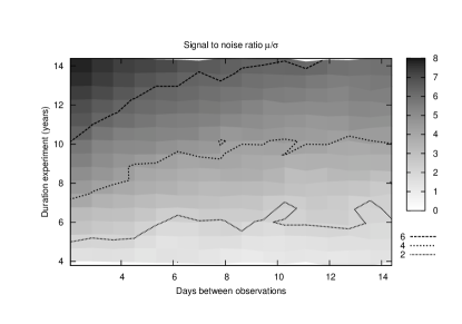
approximation. Our results, represented as signal-to-noise contour plots
for pairs of the input parameters, can be seen in
Fig. 6—Fig. 12.


5.4 Comparison to other work
More then a decade ago, McHugh et al. (1996) used a Bayesian technique to produce upper limits on the GWB using pulsar timing111We thank the anonymous referee for attracting our attention to this paper.. We found the presentation of this work rather difficult to follow. Nonetheless, it is clear that the analysis presented here is more general than that of McHugh et al.: we treat the whole pulsar array, and not just a single pulsar; we take into account the extreme redness of the noise and develop the formalism to treat the systematic errors like quadratic spindown.
Simultaneously with our work, a paper by Anholm et al. (2008, A08) has appeared on the arxiv preprint service. Their approach was to construct a quadratic estimator (written explicitly in the frequency domain), which aims to be optimally sensitive to the GWB. This improves on the original non-quadratic estimator of J05. However, a number of issues important for the pulsar timing experiment remained unaddressed, the most important among them the extreme redness of the GWB and the need to subtract consistently the quadratic spindown.
6 Conclusion
In this paper we have introduced a practical Bayesian algorithm for
measuring the GWB using Pulsar Timing Arrays. Several attractive features of
the algorithm should make it useful to the PTA community:
(1) the ability to simultaneously measure the amplitude and slope of
GWB,
(2) its ability to deal with unevenly sampled datasets, and
(3) its ability to treat systematic contributions of known functional form.
From the theoretical point of view, the algorithm is guaranteed to extract
information optimally, provided that our parametrization of the timing noise
is correct.
Test runs of our algorithm have shown that the experiments signal-to-noise (S/N) ratio strongly decreases with the redness of the pulsar timing noise, and strongly increases with the duration of the PTA experiment. We have also charted the S/N dependence on the number of well-clocked pulsars and the level of their timing noise. These charts should be helpful in the design of the optimal strategy for future PTA observations.
7 Acknowledgements
We thank Dan Stinebring, Dick Manchester, George Hobbs, Russell Edwards, Rick Jenet, Ben Stappers, Jason Hessels, and Matthew Bailes for insightful discussions about the precision pulsar timing. RvH and YL thank ATNF for its annual hospitality. This research is supported by the Netherlands organisation for Scientific Research (NWO) through VIDI Grant .
Appendix A
In this Appendix we show explicitly how to perform marginalization over the nuisance parameters in Eq. (16), rewritten here for convenience:
| (33) | |||||
From here on we will assume that is independent of (a flat prior). All values are therefore equally likely for all elements of prior to the observations. This assumption is also implicitly made in the frequentist approach when fitting for these kinds of parameters as is done in popular pulsar timing packages. We now perform the marginalisation:
| (34) |
where is the dimensionality of of . The idea now is to rewrite the the exponent of Eq. (33) in such a way that we can perform a Gaussian integral with respect to (we have to get rid of the in front of ). Therefore, we will expand and complete the square with respect to :
| (35) | |||||
where we have used the substitution:
| (36) |
Using this, we can write the dependent part of the integral of Eq. (34) as a multi dimensional Gaussian integral:
| (37) | |||||
From this it follows that:
where we have absorbed all constant terms in the normalisation constant , and where we have used:
| (39) |
References
- Begelman et al. (1980) Begelman M. C., Blandford R. D., Rees M. J., 1980, Nature, 287, 307
- Brent (1973) Brent R., 1973, Algorithms for Minimization without Derivatives. Prentice-Hall, Englewood Cliffs, New Jersey
- Britton (2000) Britton M. C., 2000, 532, 1240
- Damour & Vilenkin (2005) Damour T., Vilenkin A., 2005, 71, 063510
- Detweiler (1979) Detweiler S., 1979, 234, 1100
- Efron (1979) Efron B., 1979, Ann. of Stat., 7, 1
- Estabrook & Wahlquist (1975) Estabrook F., Wahlquist H., 1975, 6, 439
- Foster & Backer (1990) Foster R., Backer D., 1990, 361, 300
- Grishchuk (2005) Grishchuk L. P., 2005, Uspekhi Fizicheskikh Nauk, 48, 1235
- Hellings & Downs (1983) Hellings R., Downs G., 1983, 265, L39
- Hobbs et al. (2006) Hobbs G. B., Edwards R. T., Manchester R. N., 2006, Mon. Not. R. Astron. Soc., 369, 655
- Jaffe & Backer (2003) Jaffe A., Backer D., 2003, 583, 616
- Jenet et al. (2005) Jenet F., Hobbs G., Lee K., Manchester R., 2005, 625, L123
- Jenet et al. (2006) Jenet F., Hobbs G., van Straten W., Manchester R., Bailes M., Verbiest J., Edwards R., Hotan A., Sarkissian J., Ord S., 2006, 653, 1571
- Kaspi et al. (1994) Kaspi V. M., Taylor J. H., Ryba M. F., 1994, 428, 713
- Lommen (2001) Lommen A. N., 2001, PhD thesis, UC Berkeley
- Maggiore (2000) Maggiore M., 2000, 331, 283
- Manchester (2006) Manchester R. N., 2006, Chinese Journal of Astronomy and Astrophysics Supplement, 6, 139
- McHugh et al. (1996) McHugh M. P., Zalamansky G., Vernotte F., Lantz E., 1996, 54, 5993
- Newman & Barkema (1999) Newman M., Barkema G., 1999, Monte Carlo Methods in Statistical Physics. Oxford University Press Inc., pp 31–86
- Phinney (2001) Phinney E. S., 2001, ArXiv Astrophysics e-prints
- Roberts et al. (1997) Roberts G., Gelman A., Gilks W., 1997, Ann. of Appl. Prob., 7, 110
- Sazhin (1978) Sazhin M., 1978, 55, 65
- Sesana et al. (2005) Sesana A., Haardt F., Madau P., Volonteri M., 2005, 22, 363
- Stappers et al. (2006) Stappers B. W., Kramer M., Lyne A. G., D’Amico N., Jessner A., 2006, Chinese Journal of Astronomy and Astrophysics Supplement, 6, 298
- Wyithe & Loeb (2003) Wyithe J., Loeb A., 2003, 595, 614