Wave splitting of Maxwell’s equations with anisotropic heterogeneous constitutive relations

Abstract

The equations for the electromagnetic field in an anisotropic media are written in a form containing only the transverse field components relative to a half plane boundary. The operator corresponding to this formulation is the electromagnetic system’s matrix. A constructive proof of the existence of directional wave-field decomposition with respect to the normal of the boundary is presented.

In the process of defining the wave-field decomposition (wave-splitting), the resolvent set of the time-Laplace representation of the system’s matrix is analyzed. This set is shown to contain a strip around the imaginary axis. We construct a splitting matrix as a Dunford-Taylor type integral over the resolvent of the unbounded operator defined by the electromagnetic system’s matrix. The splitting matrix commutes with the system’s matrix and the decomposition is obtained via a generalized eigenvalue-eigenvector procedure. The decomposition is expressed in terms of components of the splitting matrix. The constructive solution to the question on the existence of a decomposition also generates an impedance mapping solution to an algebraic Riccati operator equation. This solution is the electromagnetic generalization in an anisotropic media of a Dirichlet-to-Neumann map.

Keywords directional wave-field decomposition, wave-splitting, anisotropy, electromagnetic system’s matrix, generalized eigenvalue problem, algebraic Riccati operator equation, generalized vertical wave number.

1 Introduction

Wave field decomposition is a tool for analyzing and computing waves in a configuration characterized by a certain directionality. The wave-field decomposition, or wave splitting, has been used to separate the wave field constituents which are of importance for the analysis on a boundary, both for direct and inverse scattering problems [25, 6, 14, 11, 9, 35, 39] and for the analysis of boundary conditions (see for example [5, 27, 2, 23]).

A remaining challenge in seismic prospecting methods is to incorporate anisotropy into the analysis. The enormous data sets used for studying such inverse problems are on the border or beyond today’s computers [3]. A common method to access such problems is to use wave field approximations. Such approximations have been developed for and applied to a wide range of hyperbolic equations describing wave propopagation in isotropic media. One class of such approximations is based on a decomposition of the wave-field into up-/down-going components. Such a decomposition is usually denoted a wave splitting or a wave-field decomposition. There are essentially two types of limitations to the present theory of wave splitting: The traditional operator based approach of wave-splitting has been limited to heterogeneous isotropic materials see e.g.,  [38, 14, 9, 28] or up-/down symmetric media [16]. This method is based essentially on constructing a certain square root operator and it fails, once the media becomes inherently anisotropic. Whereas wave-splitting by spectral decomposition of a certain matrix is restricted to homogeneous or depth-independent material. Here both anisotropic and bi-anisotropic materials have been considered [12, 30].

The present paper removes both of these limitations. We present a derivation of a three dimensional wave splitting for electromagnetic fields in the presence of inherently anisotropic loss-less heterogeneous constitutive relations. We show the existence of a decomposition by a constructive argument. The decomposition is given for media with anisotropic permittivity and permeability that is described by self-adjoint, heterogeneous, positive definite matrices. These conditions are sufficient but not necessary material conditions for the resolvent set of a certain operator to contain the strip around the imaginary axis. The requirements of the material parameters, in time-Laplace domain, are corresponding to a medium with only instantaneous lossless response. The analysis which use pseudodifferential calculus is straightforward if one assumes that the material coefficients depend smoothly on the spatial variables. In order to simplify the analysis this assumption is made. Physically this should not be regarded as a restriction since the smooth functions densely approximate the square integrable ones.

The decomposition is constructed through a generalized eigenvalue-eigenvector procedure and a certain commutation of two operators. The construction of the commuting operator, the splitting matrix, is made by means of a functional analysis approach using the resolvent of the electromagnetic system’s matrix and is analyzed with pseudodifferential calculus with parameters, to prove its existence and to study its behavior. The method is a generalization of the stratified-media case first presented in [12] and extends the theory form the linear acoustic [22] case to the considerably more complex electromagnetic case. The challenge in going from the anisotropic-acoustic case to the electromagnetic case includes a more complex differential operator with a non-trivial null-space, as well as the analysis of a resolvent operator which here is the inverse of a 4x4-matrix of operators.

There is a wealth of literature on wave splitting and their applications. A few references are mentioned below. For time-domain wave-splitting see [11], where both the wave equation and the Maxwell’s equations are considered with both applications and theory. Wave-splitting in connection with Bremmer series for linear acoustics [14, 8, 9] and uniform asymptotics and normal modes [7, 15] has been used to analyze the wave-field constituents. An extension to include dispersion is presented in [28] and wave-splitting on structural elements in [21]. The square-root of a certain operator is a key step in isotropic wave-splitting this operator has been carefully studied in [17]. A reciprocity theorem approach to decomposition is used by [33]. The results for anisotropic media includes [12, 16, 22].

Applications of the existing wave-splitting techniques include several successful analyzing tools of the wave-field including Bremmer series, normal modes and uniform asymptotics. Another spin off is the development of fast numerical codes to calculate the wave fields. Among their implementations we have ‘rational approximations’ and ‘generalized screens’ and ‘multiple-forescattering-single-backscattering approximation’ [36, 18, 31, 39]. In the active field of time-reversal mirrors see e.g., [34, 40], the wave-splitting techniques have been used see e.g., [23]. It is our hope that the extension of the wave-splitting techniques to the inherently anisotropic case will provide a base for generalization of the above mentioned applications to analysis and fast numerical codes to general anisotropic media.

The present paper is organized in a set of three propositions that step by step introduce and prove the necessary properties and tools to obtain the decomposition. The analysis is preformed in the time-Laplace domain and the procedures impose limitations on the Laplace parameter. In §2 the problem is formulated after a rewriting of Maxwell’s equations to a suitable form. In §3 the properties, mostly the spectral properties, of the electromagnetic system’s matrix are stated and proved using functional analysis. The propositions impose only the natural condition that the Laplace parameter has to belong to the right-hand half plane of the complex space. In §4 the splitting matrix is constructed and several of its properties are shown. The analysis utilize that the material parameters are self-adjoint, positive, and furthermore, require a mild constraint on the Laplace parameter, in order to obtain a certain ellipticity condition that is needed in the subsequent analysis. The most important property shown in this section is that the generalized eigenvectors of the splitting matrix can be obtained explicitly in terms of the elements of the splitting matrix. In §5 the decomposition is derived in terms of the generalized eigenvectors of the splitting matrix. The last section concludes with a discussion and some observations.

Some lengthy intermediate derivations of the electromagnetic system’s matrix in §2 are detailed in Appendix A. In Appendix B the special case of an isotropic homogeneous medium is treated using the approach developed in the present paper and the results are compared with traditional methods. In Appendix C the determinant of the symbol of the electromagnetic systems matrix is given. Furthermore, explicit integrations of the resolvent in symbol representation are presented in terms of residue calculus and the integrals are stated in terms of the roots of the determinant of the principal symbol of the electromagnetic system’s matrix.

2 Directional wave-field decomposition

2.1 The two-way equations for Maxwell equations

We consider electromagnetic wave motion in heterogeneous anisotropic media with instantaneous response. Let $x\in\mathbb{R}^{3}$ be a point in space and $t\in\mathbb{R}$ is time. The media is assumed to be independent of time. The following initial conditions of the fields ensures causality,

$$E(x,t)=0\;,\ D(x,t)=0 \mbox{for}\ t<0 \mbox{and all}\ x\in\mathbb{R}^{3}\;,$$ (2.1)

$$H(x,t)=0\;,\ B(x,t)=0 \mbox{for}\ t<0 \mbox{and all}\ x\in\mathbb{R}^{3}\;.$$

where $B=$ magnetic flux density [T], $E=$ electric field strength [V/m], $D=$ electric flux density [$\mbox{C/m}^{2}$] and $H=$ magnetic field strength [A/m]. The quantities $E,D,H,B$ are all functions of space, $x\in\mathbb{R}^{3}$ and time, $t\in\mathbb{R}$, with values in $\mathbb{R}^{3}$, we return to which function spaces that they belong at a latter point in the present paper. Above we have used standard units and notation see [19].

The electromagnetic field satisfies the first-order hyperbolic system of partial differential equations in time domain, Maxwell’s equations see e.g.,  [13, 20]. We consider Maxwell’s equations in time-Laplace domain. That is,

$$\begin{split}sB+\nabla\times E&=K^{\rm e}\;,\\ -sD+\nabla\times H&=J^{\rm e}\;.\end{split}$$ (2.2)

where $J^{\rm e}=$ external electric current density [$\mbox{A/m}^{2}$] and $K^{\rm e}=$ external magnetic current density [$\mbox{V/m}^{2}$]. The external currents are applied, prescribed, sources. The causality of the field is taken into account by requiring that all field quantities are bounded functions of the time-Laplace parameter $s$, that is in general complex valued and lies in the right-hand plane $\mathrm{Re}\left\{s\right\}>0$. With the specified initial condition (2.1), we have $\partial_{t}\rightarrow s$. In this paper $x=\{x_{1},x_{2},x_{3}\}$ are right-handed orthogonal Cartesian coordinates. All the subsequent analysis is carried out in the domain of $(x,s)$ hence there is no need to distinguish between the time dependent field, $E(x,t)$, and the Laplace-parameter dependent field, $E(x,s)$.

To explicitly introduce the material parameters into the equations we assume the following constitutive relations

$$\begin{split}B(x,s)&=\mu(x)\mu_{0}H(x,s)\\ D(x,s)&=\epsilon(x)\epsilon_{0}E(x,s)\end{split}$$ (2.3)

where $\mu=$ relative anisotropic permeability tensor, $\epsilon=$ relative anisotropic permittivity tensor, $\mu_{0}=$ empty space permeability [H/m] and $\epsilon_{0}=$ empty space permittivity [F/m]. The relative permeability and permittivity are assumed to be self adjoint and positive definite $3\times 3$ tensors of second rank, that is, the media under consideration has only instantaneous response. Inserting the constitutive relations into the Maxwell equations gives

$$\begin{split}s\mu\mu_{0}H+\nabla\times E&=K^{\rm e}\;,\\ -s\epsilon\epsilon_{0}E+\nabla\times H&=J^{\rm e}\;.\end{split}$$ (2.4)

Before proceeding we re-scale and change dimension of the equations analogous to e.g., [9, p.10] to simplify the subsequent analysis:

$$c_{0}^{-2}:=\mu_{0}\epsilon_{0}\;,\ \ \acute{s}:=\frac{s}{c_{0}}\;,\ \ \acute{H}:=\sqrt{\mu_{0}}H\;,\ \ \acute{E}:=\sqrt{\epsilon_{0}}E\;,$$

$$\acute{J}^{\rm e}:=\sqrt{\mu_{0}}J^{\rm e}\;,\ \ \acute{K}^{\rm e}:=\sqrt{\epsilon_{0}}K^{\rm e}\;,$$ (2.5)

where $c_{0}$ is the speed of light in vacuum. Upon substituting (2.5) into (2.4),

$$\begin{split}\acute{s}\mu\acute{H}+\nabla\times\acute{E}&=\acute{K}^{\rm e}\;,\\ -\acute{s}\epsilon\acute{E}+\nabla\times\acute{H}&=\acute{J}^{\rm e}\;.\end{split}$$ (2.6)

All the following considerations refer to this transformed space and for notational simplicity we remove the $\acute{\cdot}$, but remember the change in dimension, in particular that $\acute{s}$ has dimension m^-1, $\acute{H}$ and $\acute{E}$ have dimension $(\mbox{J/(m}^{3}))^{1/2}$, $\acute{J}^{\rm e}$ and $\acute{K}^{\rm e}$ has dimension $(\mbox{J/(m}^{5}))^{1/2}$. The transformation above is for dimensional convenience, in particular in the calculus of pseudodifferential operators see §4.

The ‘evolution’ of the wave field in space, along a direction of preference, can be expressed in terms of the change of the wave field in the directions perpendicular to it. The direction of preference is taken to be along the $x_{3}$-axis (or ‘vertical’ axis) and the remaining (‘horizontal’) coordinates are denoted by $x_{\alpha},x_{\beta},\ \alpha,\beta\in\{1,2\}$ or $x^{\prime}=\{x_{1},x_{2}\}$ when convenient. The procedure requires a separate treatment of the vertical components of $E$ and $H$. From (2.6) we find the vertical field components to be

$$\begin{split}s\mu_{33}H_{3}&=-s\mu_{3\beta}H_{\beta}-(\nabla\times E)_{3}+K_{3}^{\rm e}\;,\\ s\epsilon_{33}E_{3}&=-s\epsilon_{3\beta}E_{\beta}+(\nabla\times H)_{3}-J_{3}^{\rm e}\;,\end{split}$$ (2.7)

where Einstein’s summation convention for Cartesian tensors are employed for repeated indices $\alpha,\beta\in\{1,2\}$, e.g., $\mu_{3\beta}H_{\beta}=\sum_{\beta=1}^{2}\mu_{3\beta}H_{\beta}$. To project out the third component of a vector we have used the subscript 3, to explicitly show the notation consider

$$(\nabla\times E)_{3}:=\partial_{1}E_{2}-\partial_{2}E_{1}\;.$$ (2.8)

Thus, Eq. (2.7) relates the vertical components of the electric and magnetic field strength to the horizontal components. The remaining equations contained in (2.6) are

$$\begin{split}s\mu_{\alpha\beta}H_{\beta}+s\mu_{\alpha 3}H_{3}+(\nabla\times E)_{\alpha}&=K_{\alpha}^{\rm e}\;,\\ -s\epsilon_{\alpha\beta}E_{\beta}-s\epsilon_{\alpha 3}E_{3}+(\nabla\times H)_{\alpha}&=J_{\alpha}^{\rm e}\;.\end{split}$$ (2.9)

By replacing $E_{3}$, $H_{3}$ in (2.9) with (2.7) we arrive (the derivation is detailed in Appendix A) to

$$(I\partial_{3}+\mathcal{A})F=N\;,$$ (2.10)

where $N$ is a linear combinations of the sources and their derivatives cf. (A.12) and where the elements of the electromagnetic field matrix, $F$, are given by

$$F_{1}:=E_{1}\;,\ F_{2}:=-E_{2}\ \ \mbox{and}\ \ F_{3}:=H_{2}\;,\ F_{4}:=H_{1}\;.$$ (2.11)

To simplify some of the following calculations we introduce the notation

$$\tilde{E}:=(E_{1},-E_{2})^{T}\ \ \mbox{and}\ \ \tilde{H}:=(H_{2},H_{1})^{T}\;.$$ (2.12)

There are several possible orderings of the transverse components of $E$, $H$ in $F$. The particular choice of combinations given in (2.11) has two advantages. First, the given choice ensures that both the matrix operators $\mathcal{A}_{12}$ and $\mathcal{A}_{21}$ are invertible. Secondly, we have that the third component of the Poynting vector, equals $(E\times\bar{H})_{3}=\tilde{E}^{T}\overline{\tilde{H}}=(F_{1},F_{2})(\bar{F}_{3},\bar{F}_{4})^{T}$, where $\bar{\cdot}$ denotes the complex conjugate. The 4x4 electromagnetic system’s matrix, $\mathcal{A}$, is here represented by four 2x2 blocks

$$\mathcal{A}=\begin{pmatrix}\mathcal{A}_{11}&\mathcal{A}_{12}\\ \mathcal{A}_{21}&\mathcal{A}_{22}\end{pmatrix}$$ (2.13)

where each block-matrix is given by

$$\begin{split}\mathcal{A}_{11}&=\mu_{33}^{-1}\left(\begin{array}[]{rr}\mu_{23}\partial_{2}&\mu_{23}\partial_{1}\\ \mu_{13}\partial_{2}&\mu_{13}\partial_{1}\end{array}\right)+\left(\begin{array}[]{rr}\partial_{1}\epsilon_{31}&-\partial_{1}\epsilon_{32}\\ -\partial_{2}\epsilon_{31}&\partial_{2}\epsilon_{32}\end{array}\right)\epsilon_{33}^{-1}\;,\\ \\ \mathcal{A}_{12}&=s\left(\begin{array}[]{rr}\nu_{22}&\nu_{21}\\ \nu_{12}&\nu_{11}\end{array}\right)-s^{-1}\left(\begin{array}[]{rr}\partial_{1}\epsilon_{33}^{-1}\partial_{1}&-\partial_{1}\epsilon_{33}^{-1}\partial_{2}\\ -\partial_{2}\epsilon_{33}^{-1}\partial_{1}&\partial_{2}\epsilon_{33}^{-1}\partial_{2}\end{array}\right)\;,\\ \\ \mathcal{A}_{21}&=s\left(\begin{array}[]{rr}\varepsilon_{11}&-\varepsilon_{12}\\ -\varepsilon_{21}&\varepsilon_{22}\end{array}\right)-s^{-1}\left(\begin{array}[]{rr}\partial_{2}\mu_{33}^{-1}\partial_{2}&\partial_{2}\mu_{33}^{-1}\partial_{1}\\ \partial_{1}\mu_{33}^{-1}\partial_{2}&\partial_{1}\mu_{33}^{-1}\partial_{1}\end{array}\right)\;,\\ \\ \mathcal{A}_{22}&=\left(\begin{array}[]{rr}\partial_{2}\mu_{32}&\partial_{2}\mu_{31}\\ \partial_{1}\mu_{32}&\partial_{1}\mu_{31}\end{array}\right)\mu_{33}^{-1}+\epsilon_{33}^{-1}\left(\begin{array}[]{rr}\epsilon_{13}\partial_{1}&-\epsilon_{13}\partial_{2}\\ -\epsilon_{23}\partial_{1}&\epsilon_{23}\partial_{2}\end{array}\right)\;,\end{split}$$ (2.14)

in which

$$\begin{split}\varepsilon_{\alpha\beta}&=\epsilon_{\alpha\beta}-\epsilon_{\alpha 3}\epsilon_{33}^{-1}\epsilon_{3\beta}\;,\\ \nu_{\alpha\beta}&=\mu_{\alpha\beta}-\mu_{\alpha 3}\mu_{33}^{-1}\mu_{3\beta}\;.\end{split}$$ (2.15)

The permeability and permittivity are symmetric, $3\times 3$ tensors of rank (tensor order) 2 that are bounded from below and from above. Hence the upper-left $2\times 2$ matrices of $\epsilon$ and $\mu$ are bounded below by the constants $\hat{\epsilon}_{0}$ and $\hat{\mu}_{0}$ respective. To show the notation we have

$$u_{\alpha}\epsilon_{\alpha\beta}\bar{u}_{\beta}\geq\hat{\epsilon}_{0}u_{\alpha}\bar{u}_{\alpha}\;,$$ (2.16)

for any complex field $u=(u_{1},u_{2})$. From the definitions of $\varepsilon_{\alpha\beta}$ and $\nu_{\alpha\beta}$ it is clear that they are symmetric matrices (since $\varepsilon$ and $\nu$ are symmetric and all elements are real valued. Furthermore, each is bounded below by the constants $\hat{\epsilon}_{1}$ and $\hat{\mu}_{1}$ respectively. This follows from the identity (summation over repeated index $\alpha,\beta\in\{1,2\}$ and $j,k\in\{1,2,3\}$)

$$v_{j}\epsilon_{jk}\bar{v}_{k}=u_{\alpha}\varepsilon_{\alpha\beta}\bar{u}_{\beta}\;,$$ (2.17)

where

$$v_{i}=u_{\alpha}(\delta_{i\alpha}-\epsilon_{33}^{-1}\epsilon_{3\alpha}\delta_{3i})\;,\ \mbox{for}\ i=\{1,2,3\}\;,$$ (2.18)

for any complex field $u$. Since $\epsilon$ is positive definite $\varepsilon$ must also be positive definite and analogously for $\mu$ and $\nu$.

2.2 Preliminaries

We consider the electromagnetic system’s matrix and other operators on Sobolev spaces. Let $\mathrm{H}^{r}(\mathbb{R}^{2};\mathbb{C})$ be the set of functions belonging to the Sobolev space of order $r\in\mathbb{N}$ with domain in $\mathbb{R}^{2}$ and values in $\mathbb{C}$, with a weighted inner product to compensate for the dimension of the derivative. To extend this scalar space to vectors we introduce the notation

$$\mathbf{H}^{r}:=\mathrm{H}^{r}(\mathbb{R}^{2};\mathbb{C}^{4})$$ (2.19)

for a $4\times 1$ matrix, with each element in the set of functions belonging to the Sobolev space of order $r$. Let $F=(\tilde{E}^{\rm a},\tilde{H}^{\rm a})$ and $G=(\tilde{E}^{\rm b},\tilde{H}^{\rm b})$. Then we define the inner product to be

$$(F,G)_{r}=\int_{\mathbb{R}^{2}}\mathrm{d}^{2}x^{\prime}\ \sum_{|k|\leq r}y_{0}^{2|k|}\left(\partial_{x^{\prime}}^{k}\overline{\tilde{E}_{1}^{\rm a}}\ \partial_{x^{\prime}}^{k}\tilde{E}_{1}^{\rm b}+\partial_{x^{\prime}}^{k}\overline{\tilde{E}_{2}^{\rm a}}\ \partial_{x^{\prime}}^{k}\tilde{E}_{2}^{\rm b}\right.\\ +\left.\partial_{x^{\prime}}^{k}\overline{\tilde{H}_{1}^{\rm a}}\ \partial_{x^{\prime}}^{k}\tilde{H}_{1}^{\rm b}+\partial_{x^{\prime}}^{k}\overline{\tilde{H}_{2}^{\rm a}}\ \partial_{x^{\prime}}^{k}\tilde{H}_{2}^{\rm b}\right)\;,$$ (2.20)

where $y_{0}$ is a constant of dimension length and it is used to normalize the change of dimension from the derivatives. All components of the field depend on $x$, but inner products and norms refer to $x^{\prime}$ and we treat $x_{3}$ as a parameter. We have adopted the multi-index notation of pseudodifferential calculus [32] above and use $k\in\mathbb{N}^{2}$ together with

$$|k|=k_{1}+k_{2}\;.$$ (2.21)

The norm corresponding to the inner product is

$$\|F\|_{r}=\sqrt{(F,F)_{r}}\;.$$ (2.22)

The set $\mathbf{H}^{r}$ with the inner product $(\cdot,\cdot)_{r}$ is a Hilbert space. For the case $r=0$ we recover the Lebesgue space of square integrable functions, $\{\mathbf{L}^{2},(\cdot,\cdot)_{0}\}$.

The analysis of unbounded operators — such as the electromagnetic system’s matrix — requires that one specifies the domain of the operator and its embedding space. Below we consider operators on the space $\{\mathbf{L}^{2},(\cdot,\cdot)_{0}\}$, that is $\mathcal{A}:\{\mathbf{L}^{2},(\cdot,\cdot)_{0}\}\rightarrow\{\mathbf{L}^{2},(\cdot,\cdot)_{0}\}$. Since the operator is an unbounded operator, we also need to specify its domain, which is $\mathbf{H}^{2}$. The domain of the operator on a space is fundamental for the analysis. Here all operators have dense domains and when necessary, with restrictions to dense subsets of the their domains for the operation under consideration to be defined. In the case of such a restriction we use the notation $\left.\mathcal{A}\right|_{q}$ for the operator restricted to this dense subset of its domain and indicate by $q$ what dense subset is understood to be the restricted domain.

One can also consider $\mathcal{A}_{s,\lambda}$ as an operator on $\{\mathbf{H}^{r},(\cdot,\cdot)_{r}\}$, (if $r>0$ this is a restriction of the operator defined above) with domain $\mathbf{H}^{r-2}$, and the analysis extends trivially to this case. An alternative method was detailed in [22], where one instead of $\mathcal{A}_{s,\lambda}$ consider the operator $\gamma^{-r}\mathcal{A}_{s,\lambda}\gamma^{r}$, where $\gamma^{r}:=(1-y_{0}^{2}\partial_{\alpha}\partial_{\alpha})^{r/2}$. The results in this paper hold also for this class of operators.

2.3 Formulation of the problem

To be able to solve the scattering process along the vertical direction separately from the scattering process in the horizontal directions, we diagonalize the operator on the left-hand side of (2.10). This procedure will possibly lead to an additional source term on the right-hand side that accounts for the coupling. To achieve this, we construct a linear operator $\mathcal{L}$ which convert two-way fields $F$ to one-way field constituents $W$, by

$$F=\mathcal{L}W\;.$$ (2.23)

We require that $\mathcal{L}$ when introduced into (2.10) gives,

$$\mathcal{L}\,(I\partial_{3}+\mathcal{V})W=-(\partial_{3}\mathcal{L})\,W+N$$ (2.24)

so as to make $\mathcal{V}$, defined by

$$\mathcal{A}\mathcal{L}=\mathcal{L}\mathcal{V}\;,$$ (2.25)

a block diagonal matrix of operators. We call $\mathcal{L}$ the composition operator, and $W$ the wave matrix. The elements of the wave matrix represent locally the down- and up-going constituents. The expression in parentheses on the left-hand side of (2.24) represents the two so-called one-way wave operators. The first term on the right-hand side of (2.24) represents the scattering due to variations of the medium properties in the vertical direction. The scattering due to variations of the medium properties in the horizontal directions is contained in $\mathcal{V}$ and, implicitly, in $\mathcal{L}$ also.

To investigate whether solutions $\{\mathcal{L},\mathcal{V}\}$ of (2.25) exist, we introduce the column matrices, or generalized eigenvectors, $\mathcal{L}^{\pm}$, according to

$$\mathcal{L}=\left(\begin{array}[]{cc}\mathcal{L}^{+}&\mathcal{L}^{-}\end{array}\right)\;.$$ (2.26)

Upon writing the block diagonal elements of $\mathcal{V}$ (generalized eigenvalues) as

$$\mathcal{V}=\left(\begin{array}[]{cc}\mathcal{S}^{+}&0\\ 0&\mathcal{S}^{-}\end{array}\right)\;.$$ (2.27)

Eqn. (2.25) decomposes into the two systems of equations

$$\mathcal{A}\mathcal{L}^{\pm}=\mathcal{L}^{\pm}\mathcal{S}^{\pm}\;,$$ (2.28)

where $\mathcal{S}^{\pm}$ are $2\times 2$ matrices. The central problem that we consider in the present paper is to show that there exists an operator pair, $\{\mathcal{L},\mathcal{V}\}$, such that the above operator equation, (2.25), is satisfied. Since the operators are unbounded we need to modify (2.25) and (2.28) with respect to the domain of the respective operator.

Note that the upper $2\times 2$ matrix of the operators $\mathcal{L}^{\pm}$ combines the transverse electric field strength, and the lower, the magnetic field strength, whereas the elements of $W$ may be physically ‘non-observable’.

We now focus on the fundamental question: Does there exist a composition operator $\mathcal{L}$ that decomposes $\mathcal{A}$ in the above sense? To begin to show that there exists such a decomposition of $\mathcal{A}$, we derive properties of the resolvent set of $\mathcal{A}$ which enable us to define a certain operator which commute with $\mathcal{A}$.

3 Properties of the $\mathcal{A}_{s,\lambda}$ operator

In this section we show that the directional decomposition of the electromagnetic field is closely related to the spectral properties of the operator $\mathcal{A}$. The definition of the splitting matrix requires that there exists a region around the imaginary axis which is free from the spectrum. We therefore state the definition of the spectra explicitly. Consider first the operator $\mathcal{A}_{s,\lambda}$ defined on $\{\mathbf{L}^{2},(\cdot,\cdot)_{0}\}$ with domain $\mathbf{H}^{2}$:

$$\mathcal{A}_{s,\lambda}=\mathcal{A}-\lambda I\ :\ \mathbf{L}^{2}\to\mathbf{L}^{2}\;.$$ (3.1)

Following [37, §5, p.253], [29, §6.5, p.412] and [41, §VIII.1, p.209], we define the spectrum of $\mathcal{A}$, for fixed $s$ as follows: if the scalar $\lambda\in\mathbb{C}$ is such that the range of $\mathcal{A}_{s,\lambda}$ is dense in $\{\mathbf{L}^{2},(\cdot,\cdot)_{0}\}$ and $\mathcal{A}_{s,\lambda}$ has a bounded inverse, $\lambda$ is in the resolvent set, $\mathrm{P}(\mathcal{A})$, of $\mathcal{A}$, and we denote this inverse by $\mathcal{A}_{s,\lambda}^{-1}$ and call it the resolvent (at $s,\lambda$) of $\mathcal{A}$. All complex numbers not in the resolvent set form a set $\mathrm{\Sigma}(\mathcal{A})$ called the spectrum of $\mathcal{A}$.

To simplify some of the upcoming calculations we use the notations

$$s=s_{\mathrm{r}}\mathrm{e}^{\mathrm{i}\sigma}=s_{\mathrm{r}}\cos{\sigma}+\mathrm{i}s_{\mathrm{r}}\sin{\sigma}\ \ \mbox{and}\ \ \lambda=\lambda_{\mathrm{R}}+\mathrm{i}\lambda_{\mathrm{I}}\;.$$ (3.2)

The following proposition gives as a corollary that there exists a strip that belongs to the resolvent set of $\mathcal{A}$.

Proposition 1.

Let $\mathcal{A}_{s,\lambda}=\mathcal{A}-\lambda$, be defined through (2.14) and (3.1). Let

$$\mathrm{Q}:=\left\{\{s,\lambda\}\in\mathbb{C}^{2}:\mathrm{Re}\left\{s\right\}>0\ \mbox{and}\ (\mathrm{Re}\left\{\lambda\right\})^{2}<(\mathrm{Re}\left\{s\right\})^{2}\hat{\epsilon}_{1}\hat{\mu}_{1}\right\}\;,$$

where $\hat{\epsilon}_{1}$ and $\hat{\mu}_{1}$ are defined in §2.1. Then for $\{s,\lambda\}\in\mathrm{Q}$, $\mathcal{A}_{s,\lambda}$

1. is bounded from below;

2. is one-to-one;

3. has dense range;

4. is closable;

5. has an inverse:

   $$\mathcal{A}^{-1}=\left(\begin{array}[]{cc}-\mathcal{A}_{21}^{-1}\left(\mathcal{A}_{22}-\lambda\right)\mathcal{E}_{s,\lambda}^{-1}&\mathcal{A}_{21}^{-1}+\mathcal{A}_{21}^{-1}\left(\mathcal{A}_{22}-\lambda\right)\mathcal{E}_{s,\lambda}^{-1}\left(\mathcal{A}_{11}-\lambda\right)\mathcal{A}_{21}^{-1}\\ \mathcal{E}_{s,\lambda}^{-1}&-\mathcal{E}_{s,\lambda}^{-1}\left(\mathcal{A}_{11}-\lambda\right)\mathcal{A}_{21}^{-1}\end{array}\right)\;,$$

   where

   $$\mathcal{E}_{s,\lambda}:=\mathcal{A}_{12}-(\mathcal{A}_{11}-\lambda)\mathcal{A}_{21}^{-1}(\mathcal{A}_{22}-\lambda)\;.$$

Remark 1.1.

The Hilbert identity or the (first) resolvent equation,

$$\mathcal{A}_{s,\lambda}^{-1}-\mathcal{A}_{s,\lambda^{\prime}}^{-1}=(\lambda-\lambda^{\prime})\mathcal{A}_{s,\lambda}^{-1}\mathcal{A}_{s,\lambda^{\prime}}^{-1}\;,$$

for $\{s,\lambda\},\{s,\lambda^{\prime}\}\in\mathrm{Q}$. If the operator is closed and if $\{s,\lambda\}\in\mathrm{Q}$ then the resolvent is well defined and it is an analytic function of $\lambda$ (cf.  [24, §III.6.1, pp.172-174], [41, §VIII.2, pp.211-212] and [1, p.84 §3.7.5]).

Remark 1.2.

The underlying requirement of self-adjoint material parameters can be replaced by positivity of the real part of the eigenvalues of the two matrices $s\mu$, $s\epsilon$ in the case of up/down symmetric materials, i.e. when $\mu_{3\alpha}=\mu_{\alpha 3}=0$ and $\epsilon_{3\alpha}=\epsilon_{\alpha 3}=0$, for $\alpha=1,2$. This follows directly from the proof of part 1. It is not clear that this extension is valid for the general anisotropic case, we do not pursue this since our proof of Proposition 2 makes use of the self adjoint property of $\epsilon,\mu$.

From Proposition 1 it directly follows that:

Corollary 1.1.

For any fixed $s\in\mathbb{C}$ such that $\mathrm{Re}\left\{s\right\}>0$ the resolvent set of the electromagnetic system’s matrix contains the strip of all $\lambda\in\mathbb{C}$ such that

$$(\mathrm{Re}\left\{\lambda\right\})^{2}<(\mathrm{Re}\left\{s\right\})^{2}\hat{\epsilon}_{1}\hat{\mu}_{1}\;.$$ (3.3)

That is, the strip belongs to the resolvent set, $\mathrm{P}(\mathcal{A})$.

Remark 1.3.

Let $\mathcal{A}^{*}$ be the adjoint of $\mathcal{A}$ with respect to the standard inner product in $\mathbf{L}^{2}$, denote the spectrum of $\mathcal{A}$ by $\Sigma(\mathcal{A})$, and recall the relation $\Sigma(\mathcal{A})=\overline{\Sigma(\mathcal{A}^{*})}$. Let

$$J=\begin{pmatrix}0&I\\ -I&0\end{pmatrix},$$ (3.4)

where $I$ is $2\times 2$ unit matrices. From (A.13) we note that $\mathcal{A}$ satisfy the identity

$$\mathcal{A}(s)-\lambda=J^{-1}(\mathcal{A}(\bar{s}))^{*}J^{*}-\lambda=J(-(\mathcal{A}(\bar{s}))^{*}-\lambda)J^{*}\;,$$ (3.5)

and consequently when $\lambda\in\Sigma(\mathcal{A}(s))$ then $-\bar{\lambda}\in\Sigma(\mathcal{A}(\bar{s}))$.

Proof of Corollary (1.1).

Given $\mathrm{Re}\left\{s\right\}>0$, and the strip (3.3) we find such $(s,\lambda)\in\mathrm{Q}$, and hence $\mathcal{A}$ satisfy the properties 1–3 of Proposition 1. These properties are the conditions needed for a point $\lambda$ to be in the resolvent set. ∎

3.1 Properties of a quadratic form

To prove Proposition 1 we introduce some properties on an auxiliary quantity, a quadratic form, $\mathcal{C}_{s,\lambda}[F]$, defined in Lemma 1.1. Using the notation introduced in Proposition 1 and in the definition of the norm in (2.22), we have:

Lemma 1.1.

Let $\{s,\lambda\}\in\mathrm{Q}$ and define the quadratic form

$$\mathcal{C}_{s,\lambda}[F]:=\int_{\mathbb{R}^{2}}s\varepsilon_{\alpha\beta}\bar{E}_{\alpha}E_{\beta}+s^{-1}\mu_{33}^{-1}\left|(\nabla\times E)_{3}\right|^{2}\\ +s\nu_{\alpha\beta}\bar{H}_{\alpha}H_{\beta}+s^{-1}\epsilon_{33}^{-1}\left|(\nabla\times H)_{3}\right|^{2}-2\lambda\mathrm{Re}\left\{E_{1}\bar{H}_{2}-E_{2}\bar{H}_{1}\right\}+\\ 2\mathrm{i}\mu_{33}^{-1}\mathrm{Im}\left\{(\nabla\times E)_{3}\mu_{3\alpha}\bar{H}_{\alpha}\right\}+2\mathrm{i}\epsilon_{33}^{-1}\mathrm{Im}\left\{\epsilon_{\alpha 3}\bar{E}_{\alpha}(\nabla\times H)_{3}\right\}\,\mathrm{d}^{2}x^{\prime}\ \;.$$

where $F=(\tilde{E},\tilde{H})^{T}$. Then $\mathcal{C}_{s,\lambda}$ is well defined for $F\in\mathbf{H}^{1}$ and

$$|\mathcal{C}_{s,\lambda}\tilde{H}^{*}[F]|\geq C_{0}(s,\lambda)\|F\|_{0}^{2}\;,$$

where $C_{0}(s,\lambda)>0$ for $\{s,\lambda\}\in\mathrm{Q}$.

Proof.

That $\mathcal{C}_{s,\lambda}$ is well defined for $F\in\mathbf{H}^{1}$ is clear as the quadratic form contain at most one derivative for each field component in each term. To see that $\mathcal{C}_{s,\lambda}$ is bounded from below we take the real part of the integrand and using the notation introduced in (3.2) we obtain

$$(s_{\mathrm{r}}\cos\sigma)\varepsilon_{\alpha\beta}\bar{E}_{\alpha}E_{\beta}+(s_{\mathrm{r}}^{-1}\cos\sigma)\mu_{33}^{-1}\left|(\nabla\times E)_{3}\right|^{2}+(s_{\mathrm{r}}\cos\sigma)\nu_{\alpha\beta}\bar{H}_{\alpha}H_{\beta}\\ +(s_{\mathrm{r}}^{-1}\cos\sigma)\epsilon_{33}^{-1}\left|(\nabla\times H)_{3}\right|^{2}-2\lambda_{\mathrm{R}}\mathrm{Re}\left\{E_{1}\bar{H}_{2}-E_{2}\bar{H}_{1}\right\}\;,$$ (3.6)

due to that $\varepsilon$ and $\nu$ are self-adjoint. Since $\{s,\lambda\}\in\mathrm{Q}$, it follows that $\cos\sigma>0$ and we have

$$\mbox{\eqref{Eeq:qd2}}\geq s_{\mathrm{r}}\cos\sigma\left(\varepsilon_{\alpha\beta}\bar{E}_{\alpha}E_{\beta}+\nu_{\alpha\beta}\bar{H}_{\alpha}H_{\beta}\right)-2\lambda_{\mathrm{R}}\mathrm{Re}\left\{E_{1}\bar{H}_{2}-E_{2}\bar{H}_{1}\right\}\;.$$ (3.7)

For all $\eta>0$ we have the inequality

$$2\lambda_{\mathrm{R}}\mathrm{Re}\left\{E_{1}\bar{H}_{2}-E_{2}\bar{H}_{1}\right\}=2\lambda_{\mathrm{R}}\mathrm{Re}\left\{\tilde{E}^{T}\overline{\tilde{H}}\right\}\leq\eta\hat{\epsilon}_{1}|\tilde{E}|^{2}s_{\mathrm{r}}\cos\sigma+\frac{\lambda_{\mathrm{R}}^{2}}{\eta\hat{\epsilon}_{1}s_{\mathrm{r}}\cos\sigma}|\tilde{H}|^{2}\;,$$

which implies

$$\mbox{\eqref{Eeq:qd3}}\geq\hat{\epsilon}_{1}s_{\mathrm{r}}\cos\sigma(1-\eta)|\tilde{E}|^{2}+\left(\hat{\mu}_{1}s_{\mathrm{r}}\cos\sigma-\frac{\lambda_{\mathrm{R}}^{2}}{\eta\hat{\epsilon}_{1}s_{\mathrm{r}}\cos{\sigma}}\right)|\tilde{H}|^{2}\;.$$ (3.8)

Thus we require that $\eta\in(0,1)$. The largest $|\lambda_{\mathrm{R}}|$-strip is obtained in the limit $\eta\rightarrow 1$, thus

$$\lambda_{\mathrm{R}}^{2}<(\mathrm{Re}\left\{s\right\})^{2}\hat{\epsilon}_{1}\hat{\mu}_{1}\;.$$ (3.9)

Hence for given fixed $s$ such that $\mathrm{Re}\left\{s\right\}>0$ and for a fixed $\lambda$ that fulfils (3.9), there exists an optimal $\eta$ such that the bound from below in (3.8) is maximal. Thus the best choice of bound from below with the given estimates is

$$C_{0}(s,\lambda)=\max_{0<\eta<1}\min\left(\mathrm{Re}\left\{s\right\}\hat{\epsilon}_{1}(1-\eta),\left(\hat{\mu}_{1}\mathrm{Re}\left\{s\right\}-\frac{\lambda_{\mathrm{R}}^{2}}{\eta\hat{\epsilon}_{1}\mathrm{Re}\left\{s\right\}}\right)\right)>0\;.$$ (3.10)

We note that the argument above is a continuous function of $\eta$ on $[0,1]$, and the maximal-value is attained (no need for $\sup$) in the interior of the interval. Furthermore, the optimal value $\eta$ for which the $C_{0}(s,\lambda)$ is obtained as a solution of a second order equation in $\eta$, but here it suffices to know that it exists and is positive. Upon integration we find that

$$|\mathcal{C}_{s,\lambda}[F]|\geq C_{0}(s,\lambda)(\|\tilde{E}\|_{0}^{2}+\|\tilde{H}\|_{0}^{2})=C_{0}(s,\lambda)\|F\|_{0}^{2}\;.\qed$$

3.2 Proof of Proposition 1, part 1

To start the proof that the operator $\mathcal{A}_{s,\lambda}$ is bounded from below, we employ Schwartz’ inequality

$$\|\mathcal{A}_{s,\lambda}F\|_{0}\|F\|_{0}=\|K\mathcal{A}_{s,\lambda}F\|_{0}\|F\|_{0}\geq\left|(F,K\mathcal{A}_{s,\lambda}F)_{0}\right|\;,$$ (3.11)

with $F\in\mathrm{D}(\mathcal{A})=\mathbf{H}^{2}$ and where

$$K=\left(\begin{array}[]{cc}0&I\\ I&0\end{array}\right)\;,$$ (3.12)

and $I$ is a $2\times 2$-matrix. $K$ is a unitary for $\|\cdot\|_{0}$. On the block element level where $F=(\tilde{E},\tilde{H})$ (cf.  (2.12) we have

$$\bar{F}_{q}(K(\mathcal{A}-\lambda)F)_{q}=\tilde{E}^{*}\mathcal{A}_{21}\tilde{E}+\tilde{H}^{*}\mathcal{A}_{12}\tilde{H}-2\lambda\mathrm{Re}\left\{\tilde{E}^{*}\tilde{H}\right\}+\tilde{E}^{*}\mathcal{A}_{22}\tilde{H}+\tilde{H}^{*}\mathcal{A}_{11}\tilde{E}\;,$$

where the repeated index $q$ indicates summation over the four components and $\tilde{E}^{*}$ = $(\overline{\tilde{E}})^{T}$. The first term becomes after integration over $x^{\prime}$ and integration by parts,

$$\int_{\mathbb{R}^{2}}\tilde{E}^{*}\mathcal{A}_{21}\tilde{E}\,\mathrm{d}^{2}x^{\prime}\ =\int_{\mathbb{R}^{2}}s\varepsilon_{\alpha\beta}\bar{E}_{\alpha}E_{\beta}+s^{-1}\mu_{33}^{-1}\left|(\nabla\times E)_{3}\right|^{2}\,\mathrm{d}^{2}x^{\prime}\$$ (3.13)

and the second becomes

$$\int_{\mathbb{R}^{2}}\tilde{H}^{*}\mathcal{A}_{12}\tilde{H}\,\mathrm{d}^{2}x^{\prime}\ =\int_{\mathbb{R}^{2}}s\nu_{\alpha\beta}\bar{H}_{\alpha}H_{\beta}+s^{-1}\epsilon_{33}^{-1}\left|(\nabla\times H)_{3}\right|^{2}\,\mathrm{d}^{2}x^{\prime}\ \;.$$ (3.14)

The fourth term becomes after simplification and integration by parts

$$\int_{\mathbb{R}^{2}}\tilde{E}^{*}\mathcal{A}_{22}\tilde{H}\,\mathrm{d}^{2}x^{\prime}\ =\int_{\mathbb{R}^{2}}\epsilon_{33}^{-1}\epsilon_{\alpha 3}\bar{E}_{\alpha}(\nabla\times H)_{3}-(\nabla\times\bar{E})_{3}\mu_{33}^{-1}\mu_{3\alpha}H_{\alpha}\,\mathrm{d}^{2}x^{\prime}\ \;,$$ (3.15)

and the last term

$$\int_{\mathbb{R}^{2}}\tilde{H}^{*}\mathcal{A}_{11}\tilde{E}\,\mathrm{d}^{2}x^{\prime}\ =\int_{\mathbb{R}^{2}}(\nabla\times E)_{3}\mu_{33}^{-1}\mu_{\alpha 3}\bar{H}_{\alpha}-\epsilon_{33}^{-1}\epsilon_{3\alpha}E_{\alpha}(\nabla\times\bar{H})_{3}\,\mathrm{d}^{2}x^{\prime}\ \;.$$ (3.16)

Since $\epsilon$ and $\mu$ are self-adjoint matrices the two terms in (3.15) and (3.16) combine to

$$\int_{\mathbb{R}^{2}}2\mathrm{i}\mathrm{Im}\left\{\tilde{E}^{*}\mathcal{A}_{22}\tilde{H}\right\}\,\mathrm{d}^{2}x^{\prime}\ =\int_{\mathbb{R}^{2}}2\mathrm{i}\mu_{33}^{-1}\mathrm{Im}\left\{(\nabla\times\bar{E})_{3}\mu_{\alpha 3}H_{\alpha}\right\}\\ +2\mathrm{i}\epsilon_{33}^{-1}\mathrm{Im}\left\{\epsilon_{\alpha 3}\bar{E}_{\alpha}(\nabla\times H)_{3}\right\}\,\mathrm{d}^{2}x^{\prime}\ \;.$$ (3.17)

Thus,

$$\left|(F,K\mathcal{A}F)_{0}\right|=|\mathcal{C}_{s,\lambda}[F]|\;,$$ (3.18)

for $F\in\mathrm{D}(\mathcal{A}_{s,\lambda})\subset\mathbf{H}^{1}$. By Lemma 1.1 and (3.11) we obtain

$$\|\mathcal{A}F\|_{0}\geq C_{0}(s,\lambda)\|F\|_{0}\;,$$ (3.19)

where $C_{0}(s,\lambda)$ is defined in the lemma, and $C_{0}(s,\lambda)>0$ for $\{s,\lambda\}\in\mathrm{Q}$. ∎

3.3 Proof of Proposition 1, part 2

The inequality

$$\|\mathcal{A}_{s,\lambda}F\|_{0}\geq C_{0}(s,\lambda)\|F\|_{0}\;,$$ (3.20)

with $C_{0}>0$ from part 1, implies that the null space only contains the zero element. By [29, p.171, theorem 4.4.1] an operator with trivial null space is one-to-one (injective). Hence, the operator $\mathcal{A}_{s,\lambda}$ is one-to-one for $\{s,\lambda\}\in\mathrm{Q}$. ∎

3.4 Proof of Proposition 1, part 3

Let $\mathcal{A}_{s,\lambda}^{*}$ denote the adjoint of $\mathcal{A}_{s,\lambda}$ on $\mathbf{L}^{2}$. To show that the operator has dense range it is sufficient to show that the kernel of $\mathcal{A}_{s,\lambda}^{*}$ is trivial. That is,

$$\mathcal{A}_{s,\lambda}^{*}G=0\ ,\ G\in\mathrm{D}(\mathcal{A}^{*})\ \Rightarrow\ G=0\;,$$ (3.21)

thus if $\mathcal{A}_{s,\lambda}^{*}$ is bounded from below then the desired result follows directly, cf. Proposition 1, part 2.

The adjoint of $\mathcal{A}_{s,\lambda}$ with respect to the inner product $(\cdot,\cdot)_{0}$ is

$$\mathcal{A}_{s,\lambda}^{*}=\left(\begin{array}[]{cc}\mathcal{A}_{11}^{*}-\bar{\lambda}I&\mathcal{A}_{21}^{*}\\ \mathcal{A}_{12}^{*}&\mathcal{A}_{22}^{*}-\bar{\lambda}I\end{array}\right)\;,$$ (3.22)

where

$$\mathcal{A}_{11}^{*} =-\left(\begin{array}[]{rr}\partial_{2}\bar{\mu}_{23}&\partial_{2}\bar{\mu}_{13}\\ \partial_{1}\bar{\mu}_{23}&\partial_{1}\bar{\mu}_{13}\end{array}\right)\mu_{33}^{-1}-\epsilon_{33}^{-1}\left(\begin{array}[]{rr}\bar{\epsilon}_{31}\partial_{1}&-\bar{\epsilon}_{31}\partial_{2}\\ -\bar{\epsilon}_{32}\partial_{1}&\bar{\epsilon}_{32}\partial_{2}\end{array}\right)\;,$$

$$\mathcal{A}_{12}^{*} =\bar{s}\left(\begin{array}[]{rr}\bar{\nu}_{22}&\bar{\nu}_{12}\\ \bar{\nu}_{21}&\bar{\nu}_{11}\end{array}\right)-\bar{s}^{-1}\left(\begin{array}[]{rr}\partial_{1}\bar{\epsilon}_{33}^{-1}\partial_{1}&-\partial_{1}\bar{\epsilon}_{33}^{-1}\partial_{2}\\ -\partial_{2}\bar{\epsilon}_{33}^{-1}\partial_{1}&\partial_{2}\bar{\epsilon}_{33}^{-1}\partial_{2}\end{array}\right)\;,$$

$$\mathcal{A}_{21}^{*} =\bar{s}\left(\begin{array}[]{rr}\bar{\varepsilon}_{11}&-\bar{\varepsilon}_{21}\\ -\bar{\varepsilon}_{12}&\bar{\varepsilon}_{22}\end{array}\right)-\bar{s}^{-1}\left(\begin{array}[]{rr}\partial_{2}\bar{\mu}_{33}^{-1}\partial_{2}&\partial_{2}\bar{\mu}_{33}^{-1}\partial_{1}\\ \partial_{1}\bar{\mu}_{33}^{-1}\partial_{2}&\partial_{1}\bar{\mu}_{33}^{-1}\partial_{1}\end{array}\right)\;,$$

$$\mathcal{A}_{22}^{*} =-\mu_{33}^{-1}\left(\begin{array}[]{rr}\bar{\mu}_{32}\partial_{2}&\bar{\mu}_{32}\partial_{1}\\ \bar{\mu}_{31}\partial_{2}&\bar{\mu}_{31}\partial_{1}\end{array}\right)-\left(\begin{array}[]{rr}\partial_{1}\bar{\epsilon}_{13}&-\partial_{1}\bar{\epsilon}_{23}\\ -\partial_{2}\bar{\epsilon}_{13}&\partial_{2}\bar{\epsilon}_{23}\end{array}\right)\epsilon_{33}^{-1}\;,$$

where we have used that $\epsilon$, $\mu$ are self adjoint, and hence that their diagonals are real-valued. The domain of the adjoint is the set

$$\mathrm{D}(\mathcal{A}_{s,\lambda}^{*})=\{\ G\in\mathbf{L}^{2}:\\ \exists H\in\mathbf{L}^{2}\ \mbox{such that}\ (H,F)_{0}=(G,\mathcal{A}_{s,\lambda}F)_{0}\ \ \forall F\in\mathrm{D}(\mathcal{A}_{s,\lambda})\ \}\;.$$ (3.23)

To show that $\mathcal{A}_{s,\lambda}^{*}$ is bounded from below we will use the same method as in Proposition 1, part 1. First we need a small enough set that contains the domain; from the form of $\mathcal{A}_{s,\lambda}^{*}$ it is clear that if $G=\mathcal{A}_{s,\lambda}^{*}F\in\mathbf{L}^{2}$, then at least $F\in\mathbf{H}^{1}$. Thus the domain is contained in $\mathbf{H}^{1}$, that is

$$\mathrm{D}(\mathcal{A}_{s,\lambda}^{*})\subset\mathbf{H}^{1}\;.$$ (3.24)

To obtain the quadratic form needed to use Lemma 1.1, we once again use the Schwartz estimate. Let $G\in\mathrm{D}(\mathcal{A}_{s,\lambda}^{*})$, and $F:=KG$, where the matrix $K$ was introduced in (3.12) and is unitary on $(\cdot,\cdot)_{0}$ and has the properties $K=K^{*}=K^{-1}$ and $\|KG\|_{0}=\|G\|_{0}$. Similarly to (3.11) we find

$$\|\mathcal{A}_{s,\lambda}^{*}G\|_{0}\|G\|_{0}=\|\mathcal{A}_{s,\lambda}^{*}G\|_{0}\|F\|_{0}\geq|(F,\mathcal{A}_{s,\lambda}^{*}G)_{0}|=|(F,\mathcal{A}_{s,\lambda}^{*}KF)_{0}|=\\ |(K\mathcal{A}_{s,\lambda}F,F)_{0}|=|\overline{\mathcal{C}_{s,\lambda}[F]}|\;,$$ (3.25)

and with $F=\{\tilde{E},\tilde{H}\}$. Let $\{s,\lambda\}\in\mathrm{Q}$, from the properties of $\mathcal{C}_{s,\lambda}$, we find

$$|(F,\mathcal{A}_{s,\lambda}^{*}KF)_{0}|=|\overline{\mathcal{C}_{s,\lambda}[F]}|\geq C_{0}(s,\lambda)\|F\|_{0}^{2}=C_{0}(s,\lambda)\|G\|_{0}^{2}\;,$$ (3.26)

where $\mathcal{C}_{s,\lambda}$ is defined for $F\in\mathbf{H}^{1}$. From (3.25) and (3.24) it follows that $\mathcal{A}_{s,\lambda}^{*}$ is bounded from below for all $G\in\mathrm{D}(\mathcal{A}_{s,\lambda}^{*})\subset\mathbf{H}^{1}$. For the bound from below of $\mathcal{A}_{s,\lambda}^{*}$ it directly follows that $\mathcal{A}_{s,\lambda}^{*}$ has trivial kernel and thus $\mathcal{A}_{s,\lambda}$ has dense range for the condition of $\{s,\lambda\}\in\mathrm{Q}$. ∎

3.5 Proof of Proposition 1, part 4

In Section 4 below we consider a Dunford-Taylor integral over the resolvent and the analysis simplifies if $\mathcal{A}$ is closed. From the form of $\mathcal{A}_{s,\lambda}^{*}$ we note that $\mathrm{C}^{\infty}(\mathbb{R}^{2},\mathbb{C}^{4})\subset\mathrm{D}(\mathcal{A}_{s,\lambda}^{*})$ and hence it is densely defined for $\{s,\lambda\}\in\mathrm{Q}$ and thus, by [24, p.168, §III.5.5], the operator $\mathcal{A}_{s,\lambda}$ is closable. The closure is denoted by $\left\{\mathcal{A}_{s,\lambda}\right\}_{\mathrm{cl}}$.

The range for the closed operator is still dense in $\{\mathbf{L}^{2},(\cdot,\cdot)_{0}\}$ since

$$\mathrm{R}\left(\mathcal{A}_{s,\lambda}\right)\subset\mathrm{R}\left(\left\{\mathcal{A}_{s,\lambda}\right\}_{\mathrm{cl}}\right)\subset\mathbf{L}^{2}\;.$$ (3.27)

for $\{s,\lambda\}\in\mathrm{Q}$.

To show that the closed operator is bounded from below, we rely on Corollary VI.1.19 [24]. This corollary applies to sesquilinear forms in Hilbert spaces, but due to example 1.23 and example 1.3 in [24] we draw the conclusion that we can construct the sesquilinear form $(\mathcal{A}_{s,\lambda}F,\mathcal{A}_{s,\lambda}G)_{0}$ and that it is only closable when $\mathcal{A}_{s,\lambda}$ is closable. Thus, by the above mentioned corollary, we obtain that the closed form is bounded from below with the same constant and thus, the closed operator is bounded from below for $\{s,\lambda\}\in\mathrm{Q}$. ∎

3.6 Proof of Proposition 1, part 5

Given $(s,\lambda)\in\mathrm{Q}$ we have shown in part 1-3 that $\mathcal{A}_{s,\lambda}$ is one-to-one, has dense range and it is bounded from below. Consequently we know that the inverse exists and is unique. The operator $\mathcal{A}_{s,\lambda}$ can be explicitly inverted in terms of the inverse of two $2\times 2$ matrix operators through a quasi-diagonalization. Once again introduce the matrix $K$ (cf. (3.12)), with $K^{-1}=K$. We find

$$K\mathcal{A}_{s,\lambda}=\left(\begin{array}[]{cc}\mathcal{A}_{21}&\mathcal{A}_{22}-\lambda\\ \mathcal{A}_{11}-\lambda&\mathcal{A}_{12}\end{array}\right)\;,$$

and from the form of $\mathcal{A}_{21}$, (2.14) we find

$$|(\tilde{E},\mathcal{A}_{21}\tilde{E})_{0}| =\left|\int_{\mathbb{R}^{2}}s\varepsilon_{\alpha\beta}\bar{E}_{\alpha}E_{\beta}+s^{-1}\mu_{33}^{-1}|(\nabla\times E)_{3}|^{2}\,\mathrm{d}^{2}x^{\prime}\ \right|$$

$$\geq\mathrm{Re}\left\{s\right\}\hat{\epsilon}_{1}\|\tilde{E}\|_{0}^{2}\;,$$ (3.28)

hence the inverse exists and is bounded for $\mathrm{Re}\left\{s\right\}>0$. Thus $\mathcal{A}_{21}^{-1}$ is well defined. The operator $K\mathcal{A}_{s,\lambda}$ is then diagonalized as follows

$$K\mathcal{A}_{s,\lambda}\mathcal{T}_{2;s,\lambda}=\mathcal{T}_{1;s,\lambda}\mathcal{D}_{s,\lambda}\;,$$ (3.29)

where

$$\mathcal{T}_{1;s,\lambda}=\left(\begin{array}[]{cc}1&0\\ (\mathcal{A}_{11}-\lambda)\,\mathcal{A}_{21}^{-1}&1\end{array}\right)$$ (3.30)

and

$$\mathcal{T}_{2;s,\lambda}=\left(\begin{array}[]{cc}1&-\mathcal{A}_{21}^{-1}(\mathcal{A}_{22}-\lambda)\\ 0&1\end{array}\right)\;,$$ (3.31)

while

$$\mathcal{D}_{s,\lambda}=\left(\begin{array}[]{cc}\mathcal{A}_{21}&0\\ 0&\mathcal{E}_{s,\lambda}\end{array}\right)\;,$$ (3.32)

with

$$\mathcal{E}_{s,\lambda}=\mathcal{A}_{12}-(\mathcal{A}_{11}-\lambda)\mathcal{A}_{21}^{-1}(\mathcal{A}_{22}-\lambda)\;.$$ (3.33)

The characteristic operator, $\mathcal{E}_{s,\lambda}$, a matrix extension of the of the ‘transverse Helmholtz’ operator [14]. For each fixed $\lambda$, the operators $\mathcal{T}_{1;s,\lambda},\mathcal{T}_{2;s,\lambda}$ have the inverses:

$$\mathcal{T}_{1;s,\lambda}^{-1}=\left(\begin{array}[]{cc}1&0\\ -(\mathcal{A}_{11}-\lambda)\,\mathcal{A}_{21}^{-1}&1\end{array}\right)$$ (3.34)

and

$$\mathcal{T}_{2;s,\lambda}^{-1}=\left(\begin{array}[]{cc}1&\mathcal{A}_{21}^{-1}(\mathcal{A}_{22}-\lambda)\\ 0&1\end{array}\right)\;,$$ (3.35)

respectively. From the quasi-diagonalization (3.29) we obtain an explicit expression for $\mathcal{A}_{s,\lambda}^{-1}$ in terms of $\mathcal{E}_{s,\lambda}^{-1}$. That $\mathcal{E}_{s,\lambda}^{-1}$ is well defined follows by considering

$$|(\tilde{E},\mathcal{E}_{s,\lambda}\tilde{E})_{0}|=|(\tilde{E},\mathcal{A}_{12}\tilde{E})_{0}+((\mathcal{A}_{22}-\mathrm{i}\lambda_{I})\tilde{E},\mathcal{A}_{21}^{-1}(\mathcal{A}_{22}-\mathrm{i}\lambda_{I})\tilde{E})_{0}-\lambda_{R}^{2}(\tilde{E},\mathcal{A}_{21}^{-1}\tilde{E})_{0}|$$ (3.36)

where we have used $\mathcal{A}_{11}^{*}=-\mathcal{A}_{22}$. The bounds from below $\mathcal{A}_{12}\geq\mathrm{Re}\left\{s\right\}\hat{\mu}_{1}$ and $\mathcal{A}_{21}\geq\mathrm{Re}\left\{s\right\}\hat{\epsilon}_{1}$, gives

$$|(\tilde{E},\mathcal{E}_{s,\lambda}\tilde{E})_{0}|\geq\frac{1}{\mathrm{Re}\left\{s\right\}\hat{\epsilon}_{1}}((\mathrm{Re}\left\{s\right\})^{2}\hat{\epsilon}_{1}\hat{\mu}_{1}-\lambda_{R}^{2})\|\tilde{E}\|_{0}^{2}\;,$$ (3.37)

and since $(s,\lambda)\in\mathrm{Q}$ the bound from below is positive and $\mathcal{E}_{s,\lambda}$ is invertible. Starting from (3.29) and inverting term by term, gives

$$\mathcal{A}_{s,\lambda}^{-1}=\mathcal{T}_{2;s,\lambda}\mathcal{D}_{s,\lambda}^{-1}\mathcal{T}_{1;s,\lambda}^{-1}K=$$ (3.41)

$$\left(\begin{array}[]{cc}-\mathcal{A}_{21}^{-1}\left(\mathcal{A}_{22}-\lambda\right)\mathcal{E}_{s,\lambda}^{-1}&\mathcal{A}_{21}^{-1}+\mathcal{A}_{21}^{-1}\left(\mathcal{A}_{22}-\lambda\right)\mathcal{E}_{s,\lambda}^{-1}\left(\mathcal{A}_{11}-\lambda\right)\mathcal{A}_{21}^{-1}\\ \mathcal{E}_{s,\lambda}^{-1}&-\mathcal{E}_{s,\lambda}^{-1}\left(\mathcal{A}_{11}-\lambda\right)\mathcal{A}_{21}^{-1}\end{array}\right)\;.$$

∎

4 The Splitting Matrix

We proceed with the decomposition of the electromagnetic system’s matrix. As the spectrum is absent from the strip (see Corollary 1.1), we define a certain commuting operator through a resolvent integral, this operator will satisfy a number of properties, and will be called the splitting matrix. We note that if an operator has a spectral resolution, or even a part of the spectrum which is bounded, then one can define a projector with help of a Cauchy type integral, also called Dunford’s integral, over the resolvent with integration path around the bounded spectral region, see [24, III.6.4], and also [41, 32]. For the electromagnetic system’s matrix such information about the spectrum is not known, we do know however that the spectrum is separated into two parts by a strip around the imaginary axis. The idea here is to accomplish a decomposition by introducing an operator defined by an integral over the resolvent of $\mathcal{A}$, as to try to split the two parts we know exist, similarly to the case of bounded spectral regions. We use the Dunford-Taylor integral applied to a closed, unbounded, operator as in [4], cf. [24] for accretive operators. This theory is given only for closed paths, or absolutely bounded integrals, hence the extension needed here to non-closed paths require that we prove that the operator is well defined.

In this section we prove a number of properties of the splitting matrix, among them that it is well defined as a pseudodifferential operator with a parameter, that it is an involution, and that it commutes with the electromagnetic system’s matrix. Once the splitting matrix is shown to be well defined we derive its generalized eigenvalues and eigenvectors; the generalized eigenvectors are the key components for the decomposition detailed in the next section.

4.1 Definition of the Splitting Matrix

Given a fixed positive constant $S_{\mathrm{R}}>0$, let

$$\mathrm{Q}_{1}=\left\{\{s,\lambda\}\in\mathbb{C}^{2}:\mathrm{Re}\left\{s\right\}>S_{\mathrm{R}},\ |\arg s|<\pi/2\ \ \mbox{and}\ \ |\mathrm{Re}\left\{\lambda\right\}|<S_{\mathrm{R}}\sqrt{\hat{\epsilon}_{1}\hat{\mu}_{1}}\right\}\;.$$ (4.1)

From Proposition 1 we note that $\mathrm{Q}_{1}\subset\mathrm{Q}$, hence by Corollary 1.1 the strip $|\mathrm{Re}\left\{\lambda\right\}|<S_{\mathrm{R}}\sqrt{\hat{\epsilon}_{1}\hat{\mu}_{1}}$ belongs to the resolvent set of the electromagnetic system’s matrix. Thus we can consider the operator defined through

$$\mathcal{B}=\lim_{n\rightarrow\infty}\frac{1}{\pi\mathrm{i}}\int_{\lambda\in\mathrm{K}_{n}}\mathrm{d}\lambda\ \left(\left\{\mathcal{A}\right\}_{\mathrm{cl}}-I\lambda\right)^{-1}\;.$$ (4.2)

The spatial and time-Laplace dependence is present but not explicit in the notation. The integration path is:

$$\mathrm{K}_{n}=\left\{\lambda\in\mathbb{C}:\mathrm{Re}\left\{\lambda\right\}=\tau/2\ \ \mbox{and}\ \ |\mathrm{Im}\left\{\lambda\right\}|\leq n\right\}\;,$$ (4.3)

where

$$\tau=S_{\mathrm{R}}\sqrt{\hat{\epsilon}_{1}\hat{\mu}_{1}}\;,$$ (4.4)

and hence the integral path is in the resolvent set. Some of the considerations that follow become simpler if we consider the operators restriction to $\mathrm{C}^{\infty}(\mathbb{R}^{2},\mathbb{C}^{4})$, and similarly for any operator with the notation $\smash{\overset{\mbox{\raisebox{-1.72218pt}{$\scriptscriptstyle{\circ}$}}}{\phantom{\mathcal{S}}}}\mbox{\rule{0.0pt}{10.33327pt}}$. With the above introduction, we have the following proposition.

Proposition 2.

Let $\mathcal{B}$ be defined as in (4.2) with $\{s,\mathrm{K}_{n}\}\in\mathrm{Q}_{1}$ then $\mathcal{B}$

1. is a pseudodifferential operator with parameters of order 0;

2. has a restriction $\left.\mathcal{B}\right|_{q}$, which maps $\mathbf{H}^{q}$ into $\mathbf{H}^{q-1}$;

3. ‘commutes’ with $\mathcal{A}$ in the sense that on the set $\mathbf{H}^{3}$ we have

   $$\left.\mathcal{B}\right|_{1}\mathcal{A}=\mathcal{A}\left.\mathcal{B}\right|_{3}\;;$$

4. has a restriction, $\smash{\overset{\mbox{\raisebox{-1.72218pt}{$\scriptscriptstyle{\circ}$}}}{\mathcal{B}}}\mbox{\rule{0.0pt}{10.33327pt}}$, that is an involution;

5. has a restriction $\smash{\overset{\mbox{\raisebox{-1.72218pt}{$\scriptscriptstyle{\circ}$}}}{\mathcal{B}}}\mbox{\rule{0.0pt}{10.33327pt}}$ that has a generalized eigenvector $\smash{\overset{\mbox{\raisebox{-1.72218pt}{\hskip 1.99997pt$\scriptscriptstyle{\circ}$}}}{\mathcal{L}}}^{\pm}\mbox{\rule{0.0pt}{10.33327pt}}$; unique up to a normalization, and with a corresponding scalar ‘eigenvalue’ $\gamma=\pm 1$, satisfying the equation

   $$\smash{\overset{\mbox{\raisebox{-1.72218pt}{$\scriptscriptstyle{\circ}$}}}{\mathcal{B}}}\mbox{\rule{0.0pt}{10.33327pt}}\smash{\overset{\mbox{\raisebox{-1.72218pt}{\hskip 1.99997pt$\scriptscriptstyle{\circ}$}}}{\mathcal{L}}}^{\pm}\mbox{\rule{0.0pt}{10.33327pt}}=\gamma\smash{\overset{\mbox{\raisebox{-1.72218pt}{\hskip 1.99997pt$\scriptscriptstyle{\circ}$}}}{\mathcal{L}}}^{\pm}\mbox{\rule{0.0pt}{10.33327pt}}\;.$$

   The explicit form of $\smash{\overset{\mbox{\raisebox{-1.72218pt}{\hskip 1.99997pt$\scriptscriptstyle{\circ}$}}}{\mathcal{L}}}^{\pm}\mbox{\rule{0.0pt}{10.33327pt}}$ is

   $$\smash{\overset{\mbox{\raisebox{-1.72218pt}{\hskip 1.99997pt$\scriptscriptstyle{\circ}$}}}{\mathcal{L}}}^{\pm}\mbox{\rule{0.0pt}{10.33327pt}}=\begin{pmatrix}(\pm I+\smash{\overset{\mbox{\raisebox{-1.72218pt}{$\scriptscriptstyle{\circ}$}}}{\mathcal{B}}}\mbox{\rule{0.0pt}{10.33327pt}}_{11})\smash{\overset{\mbox{\raisebox{-1.72218pt}{\hskip 1.99997pt$\scriptscriptstyle{\circ}$}}}{\mathcal{N}}}^{\pm}\mbox{\rule{0.0pt}{10.33327pt}}\\ (\smash{\overset{\mbox{\raisebox{-1.72218pt}{$\scriptscriptstyle{\circ}$}}}{\mathcal{B}}}\mbox{\rule{0.0pt}{10.33327pt}}_{21})\smash{\overset{\mbox{\raisebox{-1.72218pt}{\hskip 1.99997pt$\scriptscriptstyle{\circ}$}}}{\mathcal{N}}}^{\pm}\mbox{\rule{0.0pt}{10.33327pt}}\end{pmatrix}\;,$$

   where $\smash{\overset{\mbox{\raisebox{-1.72218pt}{\hskip 1.99997pt$\scriptscriptstyle{\circ}$}}}{\mathcal{N}}}^{\pm}\mbox{\rule{0.0pt}{10.33327pt}}$ is a normalization in the form of invertible $2\times 2$ operator matrices;

6. has a restriction $\smash{\overset{\mbox{\raisebox{-1.72218pt}{$\scriptscriptstyle{\circ}$}}}{\mathcal{B}}}\mbox{\rule{0.0pt}{10.33327pt}}$ that is one-to-one on a core and thus its element $\smash{\overset{\mbox{\raisebox{-1.72218pt}{$\scriptscriptstyle{\circ}$}}}{\mathcal{B}}}\mbox{\rule{0.0pt}{10.33327pt}}_{21}$ is invertible on its range;

7. has ‘generalized eigenvectors’, i.e., that is the extension of $\smash{\overset{\mbox{\raisebox{-1.72218pt}{\hskip 1.99997pt$\scriptscriptstyle{\circ}$}}}{\mathcal{L}}}^{\pm}\mbox{\rule{0.0pt}{10.33327pt}}$ exists. With proper choice of normalization, $\left.\mathcal{L}^{\pm}\right|_{q}:\mathrm{H}^{q}(\mathbb{R}^{2},\mathbb{C}^{2})\rightarrow\mathbf{H}^{q-1}$.

Remark 2.1.

With the choice of $\smash{\overset{\mbox{\raisebox{-1.72218pt}{\hskip 1.99997pt$\scriptscriptstyle{\circ}$}}}{\mathcal{N}}}^{\pm}\mbox{\rule{0.0pt}{10.33327pt}}$ as $\smash{\overset{\mbox{\raisebox{-1.72218pt}{$\scriptscriptstyle{\circ}$}}}{\mathcal{B}}}\mbox{\rule{0.0pt}{10.33327pt}}_{21}^{-1}$, we identify $\smash{\overset{\mbox{\raisebox{-1.72218pt}{\hskip 1.99997pt$\scriptscriptstyle{\circ}$}}}{\mathcal{L}}}^{\pm}\mbox{\rule{0.0pt}{10.33327pt}}_{1}$ as a mapping between $\tilde{H}$ and $\tilde{E}$, i.e., an impedance mapping. The corresponding map in linear acoustic is a map between the pressure and the vertical particle velocity cf.  [22]. Both these mappings are the acoustic, and electromagnetic respective equivalent maps to a Dirichlet-to-Neumann map for the wave equation [11].

Remark 2.2.

To ensure that the above defined splitting matrix is non-trivial we have to exclude two cases: that the integral (4.2) collapses to the identity or to the zero operator. Whether this happens depends on the non-triviality of the spectrum. To ensure that this is not always the case we consider the homogeneous-isotropic case, see Appendix B where we obtain the explicit form of $\mathcal{B}$. We note that if the medium in the neighborhood of a point is isotropic, then microlocally, at that point, the operator $\mathcal{B}$ reduces to the isotropic case, which is clearly different from the identity and the zero operator, and hence $\mathcal{B}$ can not be the unity or the zero operator for such media.

4.2 Proof of Proposition 2, part 1

The operator $\mathcal{B}$ is defined through an improper integral over the resolvent. To prove that $\mathcal{B}$ is well defined as a pseudodifferential operator with parameter we consider first the parametrix of $\mathcal{A}_{s,\lambda}$ and then integrate each term of the asymptotic expansions with respect to $\lambda$ and prove that this step is well defined. Hence we obtain an asymptotic expansion for the symbol of $\mathcal{B}$, via the usual calculus of pseudodifferential operators we thus construct a well defined operator $\mathcal{B}$.

4.2.1 Pseudodifferential preliminaries

The calculus of pseudodifferential operators can be introduced by means of a Fourier transform, thus defining signs and symbols. For simplicity we use standard notation for the symbols and their compositions. Throughout this paper we use the left symbol (in the notation of [32]). The Fourier transform, $\mathcal{F}$, in the plane with respect to the first two variables $x^{\prime}=\{x_{1},x_{2}\}$ has an inverse given by

$$\tilde{E}(x,s)=\frac{1}{(2\pi)^{2}}\int_{\mathbb{R}^{2}}\mathrm{d}^{2}\xi^{\prime}\ \mathrm{e}^{\mathrm{i}\xi^{\prime}\cdot x^{\prime}}(\mathcal{F}\tilde{E})(\xi^{\prime},x_{3};s)$$ (4.5)

for the complex field $\tilde{E}\in\mathrm{L}_{2}(\mathbb{R}^{2},\mathbb{C}^{2})$. Here $\xi^{\prime}\cdot x^{\prime}=\xi_{1}x_{1}+\xi_{2}x_{2}$. To obtain the left symbol of $\mathcal{A}_{21}$ we let it act upon (4.5) and obtain that the integrand expression in front of $\mathrm{e}^{\mathrm{i}\xi^{\prime}\cdot x^{\prime}}(\mathcal{F}\tilde{E})(\xi^{\prime},x_{3},s)$ is

$$\mbox{\boldmath$a$}_{21}(x,\xi^{\prime};s)=s\begin{pmatrix}\varepsilon_{11}&-\varepsilon_{12}\\ -\varepsilon_{21}&\varepsilon_{22}\end{pmatrix}+(s\mu_{33})^{-1}\left(\begin{array}[]{rr}\xi_{2}^{2}&\xi_{1}\xi_{2}\\ \xi_{1}\xi_{2}&\xi_{1}^{2}\end{array}\right)\\ -\mathrm{i}s^{-1}\begin{pmatrix}(\partial_{2}\mu_{33}^{-1})\xi_{2}&(\partial_{2}\mu_{33}^{-1})\xi_{1}\\ (\partial_{1}\mu_{33}^{-1})\xi_{2}&(\partial_{1}\mu_{33}^{-1})\xi_{1}\end{pmatrix}\;.$$ (4.6)

This is the left symbol of $\mathcal{A}_{21}$. To find the appropriate behavior of the symbols we have to consider symbols with parameters. We consider $s$ to be a parameter of the same order as $\xi_{i}$. We hence find the principal symbol of $\mbox{\boldmath$a$}_{21}$ to be

$$\mbox{\boldmath$a$}_{21;1}(x,\xi^{\prime};s)=s\left(\begin{array}[]{rr}\varepsilon_{11}&-\varepsilon_{12}\\ -\varepsilon_{21}&\varepsilon_{22}\end{array}\right)+(s\mu_{33})^{-1}\left(\begin{array}[]{rr}\xi_{2}^{2}&\xi_{1}\xi_{2}\\ \xi_{1}\xi_{2}&\xi_{1}^{2}\end{array}\right)\;,$$ (4.7)

and $\mbox{\boldmath$a$}_{21;1}$ is homogeneous of order one in $(\xi^{\prime},s)$.

4.2.2 Ellipticity of $\mathcal{A}_{s,\lambda}$

For matrix valued operators it is the determinant of the symbol that controls the regularity and existence of its parametrix. We require that the coefficients to $(\xi^{\prime},s,\lambda)$ are arbitrarily smooth for each term in $\mathcal{A}_{s,\lambda}$, and thus we can use the criteria in Definition 5.1 together with Proposition $5.1^{\prime}$ of [32, pp.38,39] to define ellipticity of $\mathcal{A}_{s,\lambda}$. To construct the principal symbol of the operator $\mathcal{A}$, $\mbox{\boldmath$a$}_{;1}(x,\xi^{\prime};s)$, we proceed as above and obtain for the remaining elements

$$\mbox{\boldmath$a$}_{11;1} =\mathrm{i}\mu_{33}^{-1}\left(\begin{array}[]{rr}\mu_{23}\xi_{2}&\mu_{23}\xi_{1}\\ \mu_{13}\xi_{2}&\mu_{13}\xi_{1}\end{array}\right)+\mathrm{i}\epsilon_{33}^{-1}\left(\begin{array}[]{rr}\epsilon_{31}\xi_{1}&-\epsilon_{32}\xi_{1}\\ -\epsilon_{31}\xi_{2}&\epsilon_{32}\xi_{2}\end{array}\right)\;,$$ (4.12)

$$\mbox{\boldmath$a$}_{12;1} =s\left(\begin{array}[]{rr}\nu_{22}&\nu_{21}\\ \nu_{12}&\nu_{11}\end{array}\right)+s^{-1}\epsilon_{33}^{-1}\left(\begin{array}[]{rr}\xi_{1}^{2}&-\xi_{1}\xi_{2}\\ -\xi_{1}\xi_{2}&\xi_{2}^{2}\end{array}\right)\;,$$ (4.17)

$$\mbox{\boldmath$a$}_{22;1} =\mathrm{i}\mu_{33}^{-1}\left(\begin{array}[]{rr}\mu_{32}\xi_{2}&\mu_{31}\xi_{2}\\ \mu_{32}\xi_{1}&\mu_{31}\xi_{1}\end{array}\right)+\mathrm{i}\epsilon_{33}^{-1}\left(\begin{array}[]{rr}\epsilon_{13}\xi_{1}&-\epsilon_{13}\xi_{2}\\ -\epsilon_{23}\xi_{1}&\epsilon_{23}\xi_{2}\end{array}\right)\;.$$ (4.22)

Let

$$\mbox{\boldmath$\alpha$}_{;1}:=\mbox{\boldmath$a$}_{;1}-\lambda I.$$ (4.23)

Then $\mbox{\boldmath$\alpha$}_{;1}$ have homogeneity degree 1 in $(\xi^{\prime},s,\lambda)$. The remaining part of the symbol of $\mathcal{A}_{s,\lambda}$ has a lower degree of homogeneity in $(\xi^{\prime},s,\lambda)$. To ensure the ellipticity of an operator in the parameters $(\xi^{\prime},s,\lambda)$ the following estimate is needed

$$C_{1}(|\xi^{\prime}|^{2}+|s|^{2}+|\lambda|^{2})^{2}\leq|\det\mbox{\boldmath$\alpha$}_{;1}|\leq C_{2}(|\xi^{\prime}|^{2}+|s|^{2}+|\lambda|^{2})^{2}$$ (4.24)

for some $R$ such that $|\xi^{\prime}|^{2}+|s|^{2}+|\lambda|^{2}>R^{2}$ and with proper restrictions on the parameters $\{s,\lambda\}$. The properly supported requirement for ellipticity follows from the fact that $\mathcal{A}$ is a classical pseudodifferential operator with smooth coefficients [32]. The upper limit of (4.24) follows directly from the fact that $\det\mbox{\boldmath$\alpha$}_{;1}$ is a polynomial, homogeneous of order four in $(\xi^{\prime},s,\lambda)$ (see Appendix C), together with the fact that we can dominate this polynomial by $(|\xi^{\prime}|^{2}+|s|^{2}+|\lambda|^{2})^{2}$ and a constant, for some constant $R_{0}$ such that $|\xi^{\prime}|^{2}+|s|^{2}+|\lambda|^{2}>R_{0}^{2}$. To prove the lower limit we need a more subtle method.

The lower limit of (4.24):

This is a multi-step proof, and a complication arises since the region in $\xi^{\prime},s,\lambda$ is not conical. First we prove that the determinant is non-zero on a surface (see Figure 4.1), then we use a scaling argument to extend this to a bound from below of the form (4.24) for a conical region with the surface in figure 4.1 as ‘bottom surface’. In the last step we extend the obtained result to the non-conical domain, so as to include $\lambda_{\mathrm{R}}$.

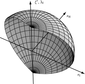
Figure 4.1: A schematic picture of the surface $|\xi^{\prime}|^{2}+|s|^{2}+|\lambda_{\mathrm{I}}|^{2}=R_{e}^{2}$, $|\arg s|<\pi/2$. In particular note that the condition $|\arg s|<\pi/2$ shrinks the surface away from a half sphere.

Non-zero determinant of $\mbox{\boldmath$\alpha$}_{;1}$

Let $\lambda_{\mathrm{R}}=0$, to explicitly show that the determinant of $\mbox{\boldmath$\alpha$}_{;1}$ is non-zero is difficult due to the large number of terms that it contains (see Appendix C). Our scaling argument needs only that the determinant is non-zero on a surface, here part of a sphere, see figure 4.1. Thus let $|s|^{2}+|\xi|^{2}+|\lambda_{\mathrm{I}}|^{2}=R_{e}^{2}$, for some positive constant $R_{e}$. We consider two cases; $s=0$ and $s\neq 0$. For the first case with $s=0$, we find from Appendix C that

$$\left.\det\mbox{\boldmath$\alpha$}_{;1}\right|_{s=0}=\\ \left(\lambda_{\mathrm{I}}^{2}-\lambda_{\mathrm{I}}\epsilon_{33}^{-1}(\epsilon_{\alpha 3}+\epsilon_{3\alpha})\xi_{\alpha}+\epsilon_{33}^{-1}\epsilon_{\alpha\beta}\xi_{\alpha}\xi_{\beta}\right)\left(\lambda_{\mathrm{I}}^{2}-\lambda_{\mathrm{I}}\mu_{33}^{-1}(\mu_{\gamma 3}+\mu_{3\gamma})\xi_{\gamma}+\mu_{33}^{-1}\mu_{\gamma\delta}\xi_{\gamma}\xi_{\delta}\right)\;.$$ (4.25)

Using the restriction that $\mu$ and $\epsilon$ are self adjoint, together with the estimate

$$2\lambda_{\mathrm{I}}\xi_{\alpha}\epsilon_{33}^{-1}\mathrm{Re}\left\{\epsilon_{3\alpha}\right\}\leq\eta_{1}^{-1}\lambda_{\mathrm{I}}^{2}+\eta_{1}\epsilon_{33}^{-2}\epsilon_{\alpha 3}\epsilon_{3\beta}\xi_{\alpha}\xi_{\beta}$$ (4.26)

for $\eta_{1}>0$ and similarly for $2\lambda_{\mathrm{I}}\mu_{33}^{-1}\mathrm{Re}\left\{\mu_{\gamma 3}\right\}\xi_{\gamma}$ gives

$$|\det\mbox{\boldmath$\alpha$}_{;1}|_{s=0} \geq\left((1-\eta_{2}^{-1})|\lambda_{\mathrm{I}}|^{2}+\mu_{33}^{-1}\nu^{(\eta_{2})}_{\alpha\beta}\xi_{\alpha}\xi_{\beta}\right)\left((1-\eta_{1}^{-1})|\lambda_{\mathrm{I}}|^{2}+\epsilon_{33}^{-1}\varepsilon^{(\eta_{1})}_{\gamma\delta}\xi_{\delta}\xi_{\gamma}\right)$$

$$\geq C_{a}\left(|\lambda_{\mathrm{I}}|^{2}+|\xi^{\prime}|^{2}\right)^{2}=\left.C_{a}R_{e}^{4}\right|_{s=0,\lambda_{R}=0}\;,$$ (4.27)

where $\left.R_{e}^{2}\right|_{s=0,\lambda_{R}=0}=|\lambda_{\mathrm{I}}|^{2}+|\xi^{\prime}|^{2}$ and

$$\varepsilon^{(\eta_{1})}_{\alpha\beta}=\epsilon_{\alpha\beta}-\eta_{1}\epsilon_{\alpha 3}\epsilon_{33}^{-1}\epsilon_{3\beta}\ \ \mbox{and}\ \ \nu^{(\eta_{2})}_{\alpha\beta}=\mu_{\alpha\beta}-\eta_{2}\mu_{\alpha 3}\mu_{33}^{-1}\mu_{3\beta}\;.$$ (4.28)

To find an explicit expression for $C_{a}$, let us choose $\eta_{1}>1$ so that

$$0<1-\eta_{1}^{-1}=\inf_{x^{\prime}}\epsilon_{33}^{-1}\inf_{|\xi^{\prime}|=1}\varepsilon^{(\eta_{1})}_{\gamma\delta}\xi_{\gamma}\xi_{\delta}\;.$$ (4.29)

The right-hand side of this equation gives the minimum of the lower eigenvalue of the matrix $\varepsilon^{(\eta_{1})}_{\gamma\delta}$ normalized with $\epsilon_{33}$. There exists an $\eta_{1}>1$ that fulfils this equation since $\hat{\epsilon}_{1}>0$, hence the left-hand side of the above expression is positive. The same way we find an $\eta_{2}>1$ such that

$$0<1-\eta_{2}^{-1}=\inf_{x^{\prime}}\mu_{33}^{-1}\inf_{|\xi^{\prime}|=1}\nu^{(\eta_{2})}_{\gamma\delta}\xi_{\gamma}\xi_{\delta}\;.$$ (4.30)

The constant $C_{a}$ becomes

$$C_{a}=(1-\eta_{1}^{-1})(1-\eta_{2}^{-1})\;.$$ (4.31)

For the case where $s\neq 0$ we use Schwartz’ inequality on an inner product. Thus we introduce the ‘matrix’ norm

$$|F|_{\rm s}^{2}=\sum_{i=1}^{4}|F_{i}|^{2}\ \ \mbox{and}\ \ |\mbox{\boldmath$\alpha$}_{;1}|_{\rm s}=\sup_{|F|_{\rm s}=1}|\mbox{\boldmath$\alpha$}_{;1}F|_{\rm s}\;,$$ (4.32)

with a corresponding inner product defined analogously and denoted by $\langle\cdot,\cdot\rangle_{\rm s}$. Both the norm and inner product depend on $(x,\xi^{\prime},s,\lambda_{\mathrm{I}},0)$. Consider the normal $4\times 4$ matrix $\mbox{\boldmath$\alpha$}_{;1}^{*}\mbox{\boldmath$\alpha$}_{;1}$, for $\lambda_{\mathrm{R}}=0$, that have eigenvalues $\kappa_{1},\ldots,\kappa_{4}$ each with a variable dependence $(x,\xi^{\prime};s,\lambda_{\mathrm{I}},0)$. From the definition of eigenvalues it follows that $0\leq\kappa_{i}\in\mathbb{R}$, where $i=1,\ldots,4$, and we use the convention $\kappa_{4}\geq\cdots\geq\kappa_{1}$. From the relation

$$\kappa_{1}^{4}\leq\kappa_{4}\kappa_{3}\kappa_{2}\kappa_{1}=\left.\det{\mbox{\boldmath$\alpha$}_{;1}^{*}\mbox{\boldmath$\alpha$}_{;1}}\right|_{\lambda_{\mathrm{R}}=0}=\left|\det{\mbox{\boldmath$\alpha$}_{;1}}\right|_{\lambda_{\mathrm{R}}=0}^{2}\;,$$ (4.33)

we find that it is enough to prove that $\kappa_{1}\neq 0$. Schwartz’ inequality (cf. (3.11)) gives

$$|\mbox{\boldmath$\alpha$}_{;1}F|_{\rm s}|F|_{\rm s}\geq|{\langle F,K\mbox{\boldmath$\alpha$}_{;1}F\rangle_{\rm s}}|\;.$$ (4.34)

Thus if for $\lambda_{\mathrm{R}}=0$ and $s\neq 0$ we can obtain an estimate of the form

$$|\langle F,K\mbox{\boldmath$\alpha$}_{;1}F\rangle_{\rm s}|\geq C_{b}|F|_{\rm s}^{2}\;,$$ (4.35)

where $C_{b}>0$, then from (4.32) and (4.35) it follows that

$$\kappa_{1}^{-1/2}=|\mbox{\boldmath$\alpha$}_{;1}^{-1}|_{\rm s}\leq C_{b}^{-1}\ \ \mbox{hence}\ \ \kappa_{1}\geq C_{b}^{2}\;.$$ (4.36)

By (4.33) we obtain,

$$\left|\det\mbox{\boldmath$\alpha$}_{;1}\right|_{\lambda_{\mathrm{R}}=0}\geq C_{b}^{4}\;,$$ (4.37)

under some restrictions on $s$, to be derived. Now with the explicit form of $\mbox{\boldmath$\alpha$}_{;1}$ we obtain

$$\left.\langle F,K\mbox{\boldmath$\alpha$}_{;1}F\rangle_{\rm s}\right|_{\lambda_{\mathrm{R}}=0}=s\left(\varepsilon_{\alpha\beta}\overline{E}_{\alpha}E_{\beta}+\nu_{\alpha\beta}\overline{H}_{\alpha}H_{\beta}\right)\\ +s^{-1}\left(\mu_{33}^{-1}\left|(\xi\times E)_{3}\right|^{2}+\epsilon_{33}^{-1}\left|(\xi\times H)_{3}\right|^{2}\right)-2\mathrm{i}\lambda_{\mathrm{I}}\mathrm{Re}\left\{E_{1}\overline{H}_{2}-E_{2}\overline{H}_{1}\right\}\\ +2\mathrm{i}\left(\mu_{33}^{-1}\mathrm{Im}\left\{(\xi\times\overline{E})_{3}\mu_{\alpha 3}H_{\alpha}\right\}+\epsilon_{33}^{-1}\mathrm{Im}\left\{\epsilon_{\alpha 3}\overline{E}_{\alpha}(\xi\times H)_{3}\right\}\right)\;,$$ (4.38)

where we have used the notation of Proof of Proposition 1, part 1. Since $s\neq 0$ we take the real part and obtain

$$|\langle F,K\mbox{\boldmath$\alpha$}_{;1}F\rangle_{\rm s}|_{\lambda_{\mathrm{R}}=0}\geq\mathrm{Re}\left\{s\right\}\left(\hat{\epsilon}_{1}|\tilde{E}|^{2}+\hat{\mu}_{1}|\tilde{H}|^{2}\right)>C_{b}|F|_{\rm s}^{2}\;,$$ (4.39)

if $\mathrm{Re}\left\{s\right\}>0$ and here

$$C_{b}=|s|\min\{\hat{\epsilon}_{1},\hat{\mu}_{1}\}\cos\sigma$$ (4.40)

is positive if $|\sigma|=|\arg s|<\pi/2$ and $s\neq 0$. By the above argument, (4.27) and (4.37) the determinant is non-zero on the surface

$$R_{e}^{2}=|\xi^{\prime}|+|s|^{2}+|\lambda_{\mathrm{I}}|^{2}\;,\ |\sigma|<\pi/2$$ (4.41)

if $R_{e}\neq 0$. Hence there exists a lower constant $C_{e}=\min(C_{b},C_{a}R_{e}^{4})$ such that

$$\left|\det\mbox{\boldmath$\alpha$}_{;1}\right|_{\lambda_{\mathrm{R}}=0}\geq C_{e}>0$$ (4.42)

on this surface.

A scaling argument:

To extend the result

$$\left|\left.\det\mbox{\boldmath$\alpha$}_{;1}(x,\xi^{\prime};s_{\mathrm{r}},\sigma,\lambda_{\mathrm{I}},\lambda_{\mathrm{R}})\right|_{\lambda_{\mathrm{R}}=0}\right|\geq C_{e}>0$$ (4.43)

for $|\xi^{\prime}|+|s|^{2}+|\lambda_{\mathrm{I}}|^{2}=R_{e}^{2}$ and $|\sigma|<\pi/2$ to a proper bound from below, we use a scaling argument. The homogeneity of $\det\mbox{\boldmath$\alpha$}_{;1}$ allow us to scale $\xi^{\prime},s,\lambda_{\mathrm{I}}$, to an arbitrary radius greater then $R_{e}$ and

$$\det\mbox{\boldmath$\alpha$}_{;1}(x,\xi^{\prime};s_{\mathrm{r}},\sigma,\lambda_{\mathrm{I}},0)=R_{e}^{-4}(|\xi^{\prime}|^{2}+|s|^{2}+|\lambda_{\mathrm{I}}|^{2})^{2}\det\mbox{\boldmath$\alpha$}_{;1}(x,\tilde{\xi^{\prime}};\tilde{s_{\mathrm{r}}},\sigma,\tilde{\lambda_{\mathrm{I}}},0)\;,$$ (4.44)

where the $\tilde{\cdot}$ variables are normalized to lie on the surface $|\xi^{\prime}|^{2}+|s|^{2}+|\lambda_{\mathrm{I}}|^{2}=R_{e}^{2}$. Thus from (4.43) we have obtained

$$\left|\det\mbox{\boldmath$\alpha$}_{;1}(x,\xi^{\prime};s_{\mathrm{r}},\sigma,\lambda_{\mathrm{I}},0)\right|\geq C_{e}R_{e}^{-4}(|\xi^{\prime}|^{2}+|s|^{2}+|\lambda_{\mathrm{I}}|^{2})^{2}\;,$$ (4.45)

in the conical domain,

$$\xi^{\prime}\in\mathbb{R}^{2}\;,\ \lambda_{\mathrm{I}}\in\mathbb{R}\;,\ s\in\mathbb{C}\ \ \mbox{and}\ \ |\arg s|<\pi/2\;,$$ (4.46)

see Figure 4.2.

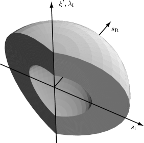
Figure 4.2: A schematic picture of the conical region in $\xi^{\prime},\ s,\ \lambda_{\mathrm{I}}$. Note that the outer surface can have an arbitrary radius larger than the inner radius $R_{e}$.

The case $\lambda_{\mathrm{R}}\neq 0$:

To extend the argument above to include the case $\lambda_{\mathrm{R}}\neq 0$ we impose the condition $\mathrm{Re}\left\{s\right\}>S_{\mathrm{R}}=\frac{1}{2}S_{R}\sqrt{\hat{\epsilon}_{1}\hat{\mu}_{1}}$. Let $\lambda_{\mathrm{R}}\leq\tau$ and $R_{e}>S_{\mathrm{R}}$. For large enough $R_{e}$, where $|\xi^{\prime}|^{2}+|s|^{2}+|\lambda_{\mathrm{I}}|^{2}\geq R_{e}^{2}$, the worst case for the bound from below of the determinant is

$$|\det\mbox{\boldmath$\alpha$}_{;1}|\geq C_{e}R_{e}^{-4}\left(|\xi^{\prime}|^{4}+|s|^{4}+|\lambda_{\mathrm{I}}|^{4}\right)-\tilde{C}_{\tau}\tau\left(|\xi^{\prime}|^{3}+|s|^{3}+|\lambda_{\mathrm{I}}|^{3}\right)$$ (4.47)

where $\tilde{C}_{\tau}$ is chosen to include the sum of the maximal material parameters in front of $\lambda_{\mathrm{R}}$. Using the Hölder and the Jensen inequalities [10, p.28, Theorem 19] gives

$$|\det\mbox{\boldmath$\alpha$}_{;1}| \geq C_{e}R_{e}^{-4}\left(|\xi^{\prime}|^{4}+|s|^{4}+|\lambda_{\mathrm{I}}|^{4}\right)-\tilde{C}_{\tau}\tau\left(|\xi^{\prime}|^{3}+|s|^{3}+|\lambda_{\mathrm{I}}|^{3}\right)$$

$$\geq C_{e}R_{e}^{-4}\left(|\xi^{\prime}|^{4}+|s|^{4}+|\lambda_{\mathrm{I}}|^{4}+|\lambda_{\mathrm{R}}|^{4}\right)-C_{\tau}\tau\left(|\xi^{\prime}|^{3}+|s|^{3}+|\lambda_{\mathrm{I}}|^{3}+|\lambda_{\mathrm{R}}|^{3}\right)$$

$$\geq C_{e}R_{e}^{-4}4^{-1}|z|^{4}-C_{\tau}\tau|z|^{3}=4^{-1}C_{e}R_{e}^{-4}|z|^{3}(|z|-4\frac{C_{\tau}R_{e}^{4}}{C_{e}}\tau)\;,$$ (4.48)

where

$$C_{\tau}=\max\{\tilde{C}_{\tau},C_{e}R_{e}^{-4}\}\;$$ (4.49)

and

$$|z|^{2}=|\xi^{\prime}|^{2}+|s|^{2}+|\lambda|^{2}\;.$$ (4.50)

Comparing with (4.24) we obtain the condition

$$C_{1}|z|^{4}\leq 4^{-1}C_{e}R_{e}^{-4}|z|^{4}-C_{\tau}|z|^{3}\tau\;.$$ (4.51)

Thus for some given, arbitrary $R_{e}>0$, there exists a large enough $R$ such that $|\det\mbox{\boldmath$\alpha$}_{;1}|>C_{1}|z|^{4}$, for $|z|^{2}>R^{2}$ when $(C_{1},R)$ satisfy the following constraints:

$$0<C_{1}<4^{-1}C_{e}R_{e}^{-4}$$ (4.52)

and

$$|z|^{2}\geq R^{2}\geq\max\{R_{0}^{2},R_{e}^{2}+\tau^{2},\left(\frac{C_{\tau}\tau}{4^{-1}C_{e}R_{e}^{-4}-C_{1}}\right)^{2}\}\;.$$ (4.53)

Hence for $\xi^{\prime}\in\mathbb{R}^{2}$ and $\{s,\lambda\}\in\mathrm{Q}_{1}$, the operator is elliptic.

Note that the quadratic form argument of Lemma 1.1 can be applied to the symbol $\mbox{\boldmath$\alpha$}_{;1}$ to yield a positive lower bound. Consequently (4.36) and (4.33) imply

$$|\det\mbox{\boldmath$\alpha$}_{;1}|\neq 0\;,$$ (4.54)

for $\{s,\lambda\}\in\mathrm{Q}$ and $|s|^{2}+|\xi^{\prime}|^{2}+|\lambda|^{2}\neq 0$. However the desired increase in $|s|^{2}+|\xi^{\prime}|^{2}+|\lambda|^{2}$ does not follow directly, since the domain is not conical. Observe also that (4.54) is true in the region $\{s,\lambda\}\in\mathrm{Q}_{1}$. This result will be used in the end of the proof of part 1.

4.2.3 The parametrix of $\mathcal{A}_{s,\lambda}$

We have above shown that $\mathcal{A}_{s,\lambda}$ is elliptic in pseudodifferential sense, hence the corresponding parametric is well defined. In the subsequent analysis we are interesting only in the principal part. From Proposition 1, part 5, we know that the inverse can be efficiently expressed in terms of $\mathcal{E}_{s,\lambda}^{-1}$ for $s,\lambda\in Q$ and different combinations of $2\times 2$ matrices. Therefore we introduce the notation of $\hat{\cdot}$ on $2\times 2$ matrices defined by

$$\hat{\mbox{\boldmath$a$}}_{21;1}:=\left(\begin{matrix}(\mbox{\boldmath$a$}_{21;1})_{22}&-(\mbox{\boldmath$a$}_{21;1})_{12}\\ -(\mbox{\boldmath$a$}_{21;1})_{21}&(\mbox{\boldmath$a$}_{21;1})_{11}\end{matrix}\right)\;,$$ (4.55)

where $(\cdot)_{ij}$ is the $(ij)$-element of the 2x2 matrix. From the definition it follows directly that

$$\hat{\hat{\mbox{\boldmath$a$}}}_{21;1}=\mbox{\boldmath$a$}_{21;1}\;,\ \ (\mbox{\boldmath$a$}_{11;1}\mbox{\boldmath$a$}_{21;1})\hat{\phantom{a}}=\hat{\mbox{\boldmath$a$}}_{21;1}\hat{\mbox{\boldmath$a$}}_{11;1}\;,$$ (4.56)

$$\ (\mbox{\boldmath$a$}_{11;1}+\mbox{\boldmath$a$}_{22;1})\hat{\phantom{a}}=\hat{\mbox{\boldmath$a$}}_{11;1}+\hat{\mbox{\boldmath$a$}}_{22;1}\;,$$ (4.57)

and

$$\hat{\mbox{\boldmath$a$}}_{21;1}\mbox{\boldmath$a$}_{21;1}=\det\mbox{\boldmath$a$}_{21;1}I\;.$$ (4.58)

The principal symbol of the characteristic operator, $\mathcal{E}_{s,\lambda}$, is

$$\mbox{\boldmath$e$}_{;1}=\mbox{\boldmath$a$}_{12;1}-(\mbox{\boldmath$a$}_{11;1}-I\lambda)\hat{\mbox{\boldmath$a$}}_{21;1}(\mbox{\boldmath$a$}_{22;1}-I\lambda)(\det\mbox{\boldmath$a$}_{21;1})^{-1}\;,$$ (4.59)

and using (4.56)–(4.57) we find

$$\hat{\mbox{\boldmath$e$}}_{;1}=\hat{\mbox{\boldmath$a$}}_{12;1}-(\hat{\mbox{\boldmath$a$}}_{22;1}-I\lambda)\mbox{\boldmath$a$}_{21;1}(\hat{\mbox{\boldmath$a$}}_{11;1}-I\lambda)(\det\mbox{\boldmath$a$}_{21;1})^{-1}\;,$$ (4.60)

thus

$$(\det\mbox{\boldmath$e$}_{;1})I=\hat{\mbox{\boldmath$e$}}_{;1}\mbox{\boldmath$e$}_{;1}\;.$$ (4.61)

From writing out all terms we find that

$$\det\mbox{\boldmath$\alpha$}_{;1}=(\det\mbox{\boldmath$e$}_{;1})(\det\mbox{\boldmath$a$}_{21;1})\;,$$ (4.62)

which is a polynomial homogeneous of order 4 in $\xi^{\prime},s,\lambda$. That $|\det\mbox{\boldmath$e$}_{;1}|\neq 0$ follows directly from that $|\det\mbox{\boldmath$\alpha$}_{;1}|\neq 0$ (see (4.54)) together with the observation that $|\det\mbox{\boldmath$a$}_{21;1}|\neq 0$ and that $|\det\mbox{\boldmath$a$}_{21;1}|$ is bounded above and below by constants times $|\xi^{\prime}|^{2}+|s|^{2}$. Hence it follows that the parametrix of $\mathcal{E}_{s,\lambda}$ is well defined. This is to be expected since the inverse of $\mathcal{E}_{s,\lambda}$ was shown to be well defined in Proposition 1, part 5. With the above consideration we find that the components of the principal symbol of the resolvent, $\mbox{\boldmath$r$}_{;-1}:=\mbox{\boldmath$\alpha$}_{;1}^{-1}=(\mbox{\boldmath$a$}-\lambda I)^{-1}$, are (cf. Proposition 1 part 5)

$$(\mbox{\boldmath$r$}_{;-1})_{11} :=-(\det\mbox{\boldmath$\alpha$}_{;1})^{-1}\hat{\mbox{\boldmath$a$}}_{21;1}(\mbox{\boldmath$a$}_{22;1}-I\lambda)\hat{\mbox{\boldmath$e$}}_{;1}\;,$$

$$\begin{split}(\mbox{\boldmath$r$}_{;-1})_{12}&:=(\det\mbox{\boldmath$a$}_{21;1})^{-1}\hat{\mbox{\boldmath$a$}}_{21;1}\big{(}I+(\det\mbox{\boldmath$\alpha$}_{;1})^{-1}(\mbox{\boldmath$a$}_{22;1}-I\lambda)\hat{\mbox{\boldmath$e$}}_{;1}(\mbox{\boldmath$a$}_{11;1}-I\lambda)\hat{\mbox{\boldmath$a$}}_{21;1}\big{)}\;,\end{split}$$

$$(\mbox{\boldmath$r$}_{;-1})_{21} :=(\det\mbox{\boldmath$\alpha$}_{;1})^{-1}\hat{\mbox{\boldmath$e$}}_{;1}(\det\mbox{\boldmath$a$}_{21;1})\;,$$ (4.63)

$$(\mbox{\boldmath$r$}_{;-1})_{22} :=-(\det\mbox{\boldmath$\alpha$}_{;1})^{-1}\hat{\mbox{\boldmath$e$}}_{;1}(\mbox{\boldmath$a$}_{11;1}-I\lambda)\hat{\mbox{\boldmath$a$}}_{21;1}\;.$$

Upon integration of the parametrix with respect to $\lambda$, the element $(\mbox{\boldmath$r$}_{;-1})_{12}$ has an unsuitable form, therefore we use the identity $\hat{\mbox{\boldmath$e$}}_{;1}\mbox{\boldmath$e$}_{;1}=I\det\mbox{\boldmath$e$}_{;1}$ and rewrite $(\mbox{\boldmath$r$}_{;-1})_{12}$ into

$$(\det\mbox{\boldmath$\alpha$}_{;1})(\mbox{\boldmath$r$}_{;-1})_{12} =\hat{\mbox{\boldmath$a$}}_{21;1}(\hat{\mbox{\boldmath$e$}}_{;1}\mbox{\boldmath$e$}_{;1}+(\det\mbox{\boldmath$a$}_{21;1})^{-1}(\mbox{\boldmath$a$}_{22;1}-I\lambda)\hat{\mbox{\boldmath$e$}}_{;1}(\mbox{\boldmath$a$}_{11;1}-I\lambda)\hat{\mbox{\boldmath$a$}}_{21;1})$$

$$=\hat{\mbox{\boldmath$a$}}_{21;1}(\hat{\mbox{\boldmath$e$}}_{;1}\mbox{\boldmath$a$}_{12;1}+(\det\mbox{\boldmath$a$}_{21;1})^{-1}[\mbox{\boldmath$a$}_{22;1},\hat{\mbox{\boldmath$e$}}_{;1}(\mbox{\boldmath$a$}_{11;1}-I\lambda)\hat{\mbox{\boldmath$a$}}_{21;1}])\;,$$ (4.64)

where $[\cdot,\cdot]$ is the standard commutator $[A,B]=AB-BA$. By inserting the explicit expression of $\hat{\mbox{\boldmath$e$}}_{;1}$ in the commutator together with the two relations $(\hat{\mbox{\boldmath$a$}}_{11;1}-I\lambda)(\mbox{\boldmath$a$}_{11;1}-I\lambda)=I\det(\mbox{\boldmath$a$}_{11;1}-I\lambda)$ and $\hat{\mbox{\boldmath$a$}}_{21;1}\mbox{\boldmath$a$}_{21;1}=\det\mbox{\boldmath$a$}_{21;1}I$ we find that (4.64) reduce to

$$(\det\mbox{\boldmath$\alpha$}_{;1})(\mbox{\boldmath$r$}_{;-1})_{12}=\hat{\mbox{\boldmath$a$}}_{21;1}(\hat{\mbox{\boldmath$e$}}_{;1}\mbox{\boldmath$a$}_{12;1}+(\det\mbox{\boldmath$a$}_{21;1})^{-1}[\mbox{\boldmath$a$}_{22;1},\hat{\mbox{\boldmath$a$}}_{12;1}(\mbox{\boldmath$a$}_{11;1}-I\lambda)\hat{\mbox{\boldmath$a$}}_{21;1}])\;.$$ (4.65)

An alternative form of (4.65) is obtain by inserting the explicit form of $\hat{\mbox{\boldmath$e$}}_{;1}$ and simplifying:

$$(\det\mbox{\boldmath$\alpha$}_{;1})(\mbox{\boldmath$r$}_{;-1})_{12}=\hat{\mbox{\boldmath$a$}}_{21;1}(I\det\mbox{\boldmath$a$}_{12;1}-(\det\mbox{\boldmath$a$}_{21;1})^{-1}(\hat{\mbox{\boldmath$a$}}_{22;1}-I\lambda)\mbox{\boldmath$a$}_{21;1}(\hat{\mbox{\boldmath$a$}}_{11;1}-I\lambda)\mbox{\boldmath$a$}_{12;1}\\ +(\det\mbox{\boldmath$a$}_{21;1})^{-1}[\mbox{\boldmath$a$}_{22;1},\hat{\mbox{\boldmath$a$}}_{12;1}(\mbox{\boldmath$a$}_{11;1}-I\lambda)\hat{\mbox{\boldmath$a$}}_{21;1}])\;.$$ (4.66)

With the above expression we have obtained the principal part of the symbol of $\mathcal{A}_{s,\lambda}^{-1}$ and each term in the matrix has the form

$$\frac{\lambda^{n}}{\det\mbox{\boldmath$\alpha$}_{;1}}\;,$$

times a constant homogeneous in $\xi,s$ of order $3-n$, here $n=0,\ldots,3$. For the lower order terms we use the recursive construction formula of e.g., [32, pp.44,45 §I.5.5] to deduct that symbols of lower orders have the $\lambda$ dependence

$$\frac{\lambda^{n^{\prime}}}{(\det\mbox{\boldmath$\alpha$}_{;1})^{m}}\;,$$ (4.67)

where $4m-n^{\prime}>1$. We have above deduced the $\lambda$ dependence for all terms in the symbolic expansion of the symbol of $\mathcal{A}_{s,\lambda}^{-1}$, and furthermore, we have the principal part explicitly.

4.2.4 $\mathcal{B}$ is a pseudodifferential with parameter of order 0

Given the parametrix of the resolvent, we integrate each term of the asymptotic series with respect to $\lambda$. To validate this procedure we show below that each of the terms is finite and that the integration does not rearrange the terms with respect to order, i.e., the principal term remains the principal term. We also show that $\mathcal{B}$ is an operator corresponding to a symbol that is homogeneous of order 0 in $(\xi,s)$.

As shown in the previous section, each element of the resolvent has the form

$$\frac{\lambda^{n}}{(\det\mbox{\boldmath$\alpha$}_{;1})^{m}}\;,$$

with $4m-n\geq 1$. The principal symbol has $m=1$ and $n=0,1,2,3$, all other terms have homogeneity 0 or lower. In the evaluation of the integral we distinguish between two different cases, the principal valued integral corresponding to $n=3,m=1$ and the other cases. We observe that due to the homogeneity of the parametrix terms the case $n=3$, $m=1$ is the only principal integral.

The case $m=1$, $n=3$ gives a finite result, which we find by evaluation the integral over the integrand (4.2.4). In order to do this claim that we can use the representation

$$\det\mbox{\boldmath$\alpha$}_{;1}=(\lambda-\lambda_{1}^{+})(\lambda-\lambda_{2}^{+})(\lambda-\lambda_{1}^{-})(\lambda-\lambda_{2}^{-})\;,$$ (4.68)

where the eigenvalues, i.e., the roots of the fourth order polynomial $\det\mbox{\boldmath$\alpha$}_{;1}$, are denoted by $\lambda^{\pm}_{1},\lambda^{\pm}_{2}$ where the $+(-)$ indicates that they have positive (negative) real part. Indeed, to show that two of the eigenvalues of $\mbox{\boldmath$a$}_{;1}$ have positive(negative) real part we consider the isotropic case. The isotropic $\det\mbox{\boldmath$\alpha$}_{;1}$ have the $\lambda$-roots (cf. Appendix B)

$$\lambda=\pm\sqrt{s^{2}\epsilon^{\mathrm{iso}}\mu^{\mathrm{iso}}+|\xi|^{2}}\;,$$ (4.69)

i.e., two double roots on each side of the strip $|\mathrm{Re}\left\{\lambda\right\}|<S_{R}\inf_{x^{\prime}}\sqrt{\epsilon^{\mathrm{iso}}\mu^{\mathrm{iso}}}$. The lower bound on $\mathcal{A}_{s,\lambda}$ in Proposition 1, part 1 shows that for each anisotropic material with instantaneous response, the area around the imaginary axis is free from eigenvalues. We introduce a parameter $\gamma$ in the material coefficients by

$$\epsilon^{(\gamma)}:=\epsilon^{\rm{iso}}+\gamma(\epsilon-\epsilon^{\rm iso})$$ (4.70)

and analogously for $\mu^{(\gamma)}$. The lower bound on $\mbox{\boldmath$\alpha$}_{;1}$, that is obtained by applying Lemma 1.1 and Proposition 1, part 1-3, to $\mbox{\boldmath$\alpha$}_{;1}$, and apparent in (4.54), ensures us that for all $\gamma\in[0,1]$ the $|\det\mbox{\boldmath$\alpha$}_{;1}^{(\gamma)}|$ is bounded from below and that there are no eigenvalues on the strip around the imaginary axis, and since the eigenvalues of a matrix depend point-wise continuous on its coefficient [24, pp.107-108, §2.5.1], the eigenvalues vary continuously, but not discontinuously on each side of the imaginary axis. In the case $\gamma=0$ there are two eigenvalues on each side, by counting multiplicity and hence, by the continuity of the eigenvalues, this has to be the case for all $\gamma\in[0,1]$. Thus we have shown the claim. The symmetry of $\mathcal{A}$ discussed in Remark 1.3 can be used to show the same result for the special case $s=\mathrm{Re}\left\{s\right\}$. With the representation (4.68) we evaluate the integral

$$\lim_{n\rightarrow\infty}\int_{-n}^{n}\mathrm{d}\lambda_{\mathrm{I}}\ \frac{\lambda^{3}}{\det\mbox{\boldmath$\alpha$}_{;1}}\;,$$ (4.71)

by partial fraction decomposition. Assume initially that there are no equal roots then

$$\frac{\lambda^{3}}{\det\mbox{\boldmath$\alpha$}_{;1}}=\frac{D_{1,+}}{\lambda-\lambda_{1}^{+}}+\frac{D_{2,+}}{\lambda-\lambda_{2}^{+}}+\frac{D_{1,-}}{\lambda-\lambda_{1}^{-}}+\frac{D_{2,-}}{\lambda-\lambda_{2}^{-}}\;,$$ (4.72)

where all $D$ depended only on $\lambda_{1,2}^{\pm}$. Each such fraction is integrated over the imaginary axis to become

$$\begin{split}\lim_{n\rightarrow\infty}\int_{-n}^{n}\mathrm{d}\lambda_{\mathrm{I}}\ \frac{1}{\lambda-\lambda_{1,2}^{\pm}}&=\lim_{n\rightarrow\infty}\left.\ln(\lambda-\lambda_{1,2}^{\pm})\right|_{\lambda_{\mathrm{I}}=-n}^{\lambda_{\mathrm{I}}=n}\\ &=\mathrm{i}\pi\mathop{\mathrm{sgn}(\mathrm{Re}\left\{\lambda_{\mathrm{R}}-\lambda_{1,2}^{\pm}\right\})}=\mp\mathrm{i}\pi\;,\end{split}$$ (4.73)

where the branch cut is along the negative imaginary axis and where $|\lambda_{\mathrm{R}}|<|\mathrm{Re}\left\{\lambda_{1,2}^{\pm}\right\}|$. Concerning the choice of branch cut, observe that the integral above should be summed over each eigenvalue, thus the branch cut of the logarithm has to be chosen such that it agrees for all eigenvalues, hence the negative imaginary axis. Thus

$$\lim_{n\rightarrow\infty}\int_{-n}^{n}\mathrm{d}\lambda_{\mathrm{I}}\ \frac{\lambda^{3}}{\det\mbox{\boldmath$\alpha$}_{;1}}=\mathrm{i}\pi(D_{1,+}+D_{2,+}-D_{1,-}-D_{2,-})$$ (4.74)

for $n=0,\ldots,3$. Here

$$D_{1,+} :=\frac{(\lambda_{1}^{+})^{3}}{(\lambda_{1}^{+}-\lambda_{2}^{+})(\lambda_{1}^{+}-\lambda_{1}^{-})(\lambda_{1}^{+}-\lambda_{2}^{-})}\;,$$

$$D_{2,+} :=\frac{-(\lambda_{2}^{+})^{3}}{(\lambda_{1}^{+}-\lambda_{2}^{+})(\lambda_{2}^{+}-\lambda_{1}^{-})(\lambda_{2}^{+}-\lambda_{2}^{-})}\;,$$

$$D_{1,-} :=\frac{(\lambda_{1}^{-})^{3}}{(\lambda_{1}^{+}-\lambda_{1}^{-})(\lambda_{2}^{+}-\lambda_{1}^{-})(\lambda_{1}^{-}-\lambda_{2}^{-})}\;,$$

$$D_{2,-} :=\frac{-(\lambda_{2}^{-})^{3}}{(\lambda_{1}^{+}-\lambda_{2}^{-})(\lambda_{2}^{+}-\lambda_{2}^{-})(\lambda_{1}^{-}-\lambda_{2}^{-})}\;,$$

and each term is homogeneous of order $0$. To show that the sum is bounded from above we have to eliminate $(\lambda_{1}^{+}-\lambda_{2}^{+})$ and $(\lambda_{1}^{-}-\lambda_{2}^{-})$ from the denominator. We find that

$$D_{1,+}+D_{2,+}=\frac{\lambda_{1}^{+}\lambda_{2}^{+}(\lambda_{1}^{+}+\lambda_{2}^{+})-\lambda_{1}^{-}((\lambda_{1}^{+})^{2}+\lambda_{1}^{+}\lambda_{2}^{+}+(\lambda_{2}^{+})^{2})}{(\lambda_{1}^{+}-\lambda_{1}^{-})(\lambda_{1}^{+}-\lambda_{2}^{-})(\lambda_{2}^{+}-\lambda_{1}^{-})(\lambda_{2}^{+}-\lambda_{2}^{-})}$$ (4.75)

and

$$D_{1,-}+D_{1,-}=\frac{\lambda_{1}^{-}\lambda_{2}^{-}(\lambda_{1}^{-}+\lambda_{2}^{-})-\lambda_{1}^{+}((\lambda_{1}^{-})^{2}+\lambda_{1}^{-}\lambda_{2}^{-}+(\lambda_{2}^{-})^{2})}{(\lambda_{1}^{+}-\lambda_{1}^{-})(\lambda_{1}^{+}-\lambda_{2}^{-})(\lambda_{2}^{+}-\lambda_{1}^{-})(\lambda_{2}^{+}-\lambda_{2}^{-})}\;,$$ (4.76)

hence the denominator is bounded away from zero by $(2\tau)^{4}$, since $|\lambda_{\mathrm{R}}^{\pm}|\geq\tau=S_{R}\sqrt{\hat{\epsilon}_{1}\hat{\mu}_{1}}$, this follows from the Corollary 1.1 that shows that the strip $|\lambda_{\mathrm{R}}|<\tau$ is free from eigenvalues. Hence the integral is bounded.

The case with equal eigenvalues follows similarly. Assume $\lambda_{2}^{+}=\lambda_{1}^{+}$ and $\lambda_{1}^{-}\neq\lambda_{2}^{-}$ then

$$\frac{\lambda^{3}}{\det\mbox{\boldmath$\alpha$}_{;1}}=\frac{D_{1,+,2}}{(\lambda-\lambda_{1}^{+})^{2}}+\frac{D_{1,+,1}}{\lambda-\lambda_{1}^{+}}+\frac{D_{1,-}}{\lambda-\lambda_{1}^{-}}+\frac{D_{2,-}}{\lambda-\lambda_{2}^{-}}\;,$$ (4.77)

where

$$D_{1,+,2} :=\frac{(\lambda_{1}^{+})^{3}}{(\lambda_{1}^{+}-\lambda_{1}^{-})(\lambda_{1}^{+}-\lambda_{2}^{-})}\;,$$

$$D_{1,+,1} :=\frac{\lambda_{1}^{+}\lambda_{2}^{+}(\lambda_{1}^{+}\lambda_{2}^{+}-\lambda_{1}^{-}\lambda_{2}^{-})+(\lambda_{1}^{+}+\lambda_{2}^{+})(\lambda_{1}^{+}+\lambda_{2}^{+}\lambda_{1}^{-}\lambda_{2}^{-}-(\lambda_{1}^{-}-\lambda_{2}^{-})\lambda_{1}^{+}\lambda_{2}^{+})}{(\lambda_{1}^{+}-\lambda_{1}^{-})^{2}(\lambda_{1}^{+}-\lambda_{2}^{-})^{2}}\;.$$

With the integral

$$\lim_{n\rightarrow\infty}\int_{-n}^{n}\mathrm{d}\lambda_{\mathrm{I}}\ \frac{1}{(\lambda-\lambda_{1}^{+})^{2}}=\lim_{n\rightarrow\infty}\left.\frac{1}{\lambda_{1}^{+}-\lambda}\right|_{\lambda_{\mathrm{I}}=-n}^{\lambda_{\mathrm{I}}=n}=0$$ (4.78)

and (4.73) we find that

$$\lim_{n\rightarrow\infty}\int_{-n}^{n}\mathrm{d}\lambda_{\mathrm{I}}\ \frac{\lambda^{3}}{\det\mbox{\boldmath$\alpha$}_{;1}}=\mathrm{i}\pi(D_{1,+,1}-D_{1,-}-D_{2,-})\;,$$ (4.79)

and hence, it is bounded from above and homogeneous of order $0$. The case where $\lambda_{1}^{-}=\lambda_{2}^{-}$ and $\lambda_{2}^{+}\neq\lambda_{1}^{+}$ is totally analogous.

For the case with two equal eigenvalues we have

$$\frac{\lambda^{3}}{\det\mbox{\boldmath$\alpha$}_{;1}}=\frac{D_{+,2}}{(\lambda-\lambda_{1}^{+})^{2}}+\frac{D_{+,1}}{\lambda-\lambda_{1}^{+}}+\frac{D_{-,2}}{(\lambda-\lambda_{1}^{-})^{2}}+\frac{D_{-,1}}{\lambda-\lambda_{2}^{-}}$$ (4.80)

and from (4.73) and (4.78) we find that

$$\lim_{n\rightarrow\infty}\int_{-n}^{n}\mathrm{d}\lambda_{\mathrm{I}}\ \frac{\lambda^{3}}{\det\mbox{\boldmath$\alpha$}_{;1}}=\mathrm{i}\pi(D_{+,1}-D_{-,1})\;.$$ (4.81)

Hence we need only to find $D_{+,1}$ and $D_{-,1}$,

$$D_{+,1}=\frac{(\lambda_{1}^{+})^{2}(\lambda_{1}^{+}-3\lambda_{1}^{-})}{(\lambda_{1}^{+}-\lambda_{1}^{-})^{3}}\;,\ \ D_{-,1}=\frac{(\lambda_{1}^{-})^{2}(3\lambda_{1}^{+}-\lambda_{1}^{-})}{(\lambda_{1}^{+}-\lambda_{1}^{-})^{3}}$$

and hence the integral is homogeneous of order 0 and bounded from above since the denominator is bounded from below. We have thus shown that the integral (4.71) is well defined, and homogeneous of order 0 for all possible combinations of $\lambda$-roots in $\det\mbox{\boldmath$\alpha$}_{;1}$.

Next we show that the remaining terms have homogeneous degree +1 compared to the corresponding term in the polyhomogeneous expansion of $r$ and consequently that the integral over $\lambda$ does not rearrange the symbol expansion. From the construction of the parametrix of $\mathcal{A}_{s,\lambda}$ we know that its asymptotic symbol expansion has a $\lambda$ dependence of the form (4.67). Using that the determinant $\det\mbox{\boldmath$\alpha$}_{;1}$ is homogeneous of degree 4 in $(\xi^{\prime},s,\lambda)$, we find that

$$I_{n,m}(x,\xi^{\prime};s):=\int\mathrm{d}\lambda\ \frac{\lambda^{n}}{\left(\det\mbox{\boldmath$\alpha$}_{;1}(x,\xi^{\prime};s,\lambda)\right)^{m}}$$ (4.82)

is homogeneous of degree $n-4m+1$ if $4m-n\geq 2$. Indeed,

$$\eta^{n-4m+1}I_{n,m}(x,s;\xi^{\prime}) =\int\mathrm{d}\lambda\ \eta\frac{(\eta\lambda)^{n}}{\left(\det\mbox{\boldmath$\alpha$}_{;1}(x,\eta\xi^{\prime};\eta s,\eta\lambda)\right)^{m}}$$ (4.83)

$$=\int\mathrm{d}\tilde{\lambda}\ \frac{\tilde{\lambda}^{n}}{\left(\det\mbox{\boldmath$\alpha$}_{;1}(x,\eta\xi^{\prime};\eta s,\tilde{\lambda})\right)^{m}}=I_{n,m}(x,\eta\xi^{\prime};\eta s)\;,$$

where we have used 1) that the limits of the integral goes to infinity, 2) that the $\lambda$-roots scale with $\eta$, implying that the strip $\tilde{\lambda}_{\mathrm{R}}\leq\eta\tau$ is free from poles, 3) the scaled integration path is equivalent to the integration path of $\tilde{\lambda}_{\mathrm{R}}=\tau/2$ since $\mathcal{A}_{s,\lambda}^{-1}$ is analytical in $\lambda$ in the resolvent set and 4) that $\eta$ is such that $\eta\mathrm{Re}\left\{s\right\}>S_{\mathrm{R}}$. Thus $I_{n,m}$ is homogeneous of degree $n-4m+1$ in $\xi^{\prime},s$. Each term in the polyhomogeneous expansion of $r$ have a $\lambda$-dependence in the form of $I_{n,m}$ with a $\lambda$ independent coefficient. It follows that each integrated term of the expansion has a homogeneous degree that is one order higher than the homogeneous degree of each term of $r$.

Let

$$|z|^{2}:=|\xi^{\prime}|^{2}+|s|^{2}\;.$$

To show that each of the integrals $I_{n,m}$ is bounded from above, for fixed $\xi^{\prime},s$ such that $z\neq 0$ we use the estimate of the lower bound of the determinant for $(s,\lambda)\in Q_{1}$ (cf. §4.2.2 and (4.54)),

$$|\det\mbox{\boldmath$\alpha$}_{;1}|\geq C_{1}(|\lambda|^{2}+|z|^{2})^{2}\;.$$ (4.84)

The principal case $4m-n=1$ is taken care of above see (4.71). For $4m-n>1$ we have

$$\left|\int_{\mathbb{R}}\mathrm{d}\lambda_{\mathrm{I}}\ \frac{\lambda^{n}}{|\det\mbox{\boldmath$\alpha$}_{;1}|^{m}}\right|\leq 2C_{1}^{-m}\int_{0}^{\infty}\mathrm{d}\lambda_{\mathrm{I}}\ \frac{|\lambda|^{n}}{(|\lambda|^{2}+|z|^{2})^{2m}}\\ =2C_{1}^{-m}\left(\int_{0}^{|z|}\frac{|\lambda|^{n}}{(|\lambda|^{2}+|z|^{2})^{2m}}\mathrm{d}\lambda_{\mathrm{I}}\ +\int_{|z|}^{\infty}\frac{|\lambda|^{n}}{(|\lambda|^{2}+|z|^{2})^{2m}}\mathrm{d}\lambda_{\mathrm{I}}\ \right)\;,$$ (4.85)

where for $|\lambda_{\mathrm{I}}|<|z|$ we use

$$\frac{|\lambda|^{n}}{(|\lambda|^{2}+|z|^{2})^{2m}}\leq\frac{1}{(|z|^{2}+|\lambda_{\mathrm{R}}|^{2})^{2m-n/2}}\leq\frac{1}{|z|^{4m-n}}\;,$$ (4.86)

and for $|\lambda_{\mathrm{I}}|>|z|$ we use the estimate

$$\frac{|\lambda|^{n}}{(|\lambda|^{2}+|z|^{2})^{2}}\leq\frac{1}{(|\lambda_{\mathrm{R}}|^{2}+|\lambda_{\mathrm{I}}|^{2})^{2m-n/2}}\leq\frac{1}{|\lambda_{\mathrm{I}}|^{4m-n}}\;.$$ (4.87)

Inserting the above estimates into (4.85) yields

$$\begin{split}\left|\int_{\mathbb{R}}\mathrm{d}\lambda_{\mathrm{I}}\ \frac{\lambda^{n}}{|\det\mbox{\boldmath$\alpha$}_{;1}|^{m}}\right|&\leq 2C_{1}^{-m}\left(\frac{|z|}{|z|^{4m-n}}+\int_{|z|}^{\infty}|\lambda_{\mathrm{I}}|^{n-4m}\mathrm{d}\lambda_{\mathrm{I}}\ \right)\\ &=\frac{2}{C_{1}^{m}|z|^{4m-n-1}}\left(\frac{4m-n}{(4m-n-1)}\right)\end{split}$$ (4.88)

and hence the integral is bounded from above since $|z|>0$ and $4m-n-1>0$. Thus we find that the asymptotic series expansion of $r$ can be integrated, since each term is finite for $s>S_{R}$ and $\arg s<\pi/2$. Furthermore, the $\lambda$-integral of $\mbox{\boldmath$r$}_{-}m$, which is homogeneous of order $-m$, results in $\mbox{\boldmath$b$}_{-m+1}$ which is homogeneous of order $-m+1$. We have hence a well defined polyhomogeneous asymptotic expansion of a pseudodifferential operator with a parameter of homogeneous degree 0 in $\{\xi^{\prime},s\}$, the corresponding operator is represented in the usual way through an oscillatory integral.

One can use the residue theorem to evaluate the integrals in terms of the roots of the equation $\det\mbox{\boldmath$\alpha$}_{;1}=0$. This is done for arbitrary $I_{m,n}$, $4m-n>1$ in Appendix C.

We have above found an oscillatory integral representation of the desired operator $\mathcal{B}$ through the $\lambda$-integral of the symbol expansion of the resolvent. Its principal symbol is $\int\mathrm{d}\lambda\ \mbox{\boldmath$r$}_{;-1}$, where as usual $\mbox{\boldmath$r$}_{;-1}:=\mbox{\boldmath$\alpha$}_{;1}^{-1}=(\mbox{\boldmath$a$}-\lambda I)^{-1}$. One question remains in order to associate $\mathcal{B}$ with $\int\mathrm{d}\lambda\ \mathcal{A}_{s,\lambda}^{-1}$. It can be reduced to a question of the order of iterated integrals. Towards this end we use an alternative representation of the $\lambda$-integral. We note that

$$\int_{\lambda\in K}\mathrm{d}\lambda\ \mbox{\boldmath$\alpha$}_{;1}^{-1}=\int_{\lambda_{\mathrm{I}}\in[0,\infty],\lambda_{\mathrm{R}}\leq\tau}(\mbox{\boldmath$a$}_{;1}-I(\lambda_{\mathrm{R}}-\mathrm{i}\lambda_{\mathrm{I}}))^{-1}2(\mbox{\boldmath$a$}_{;1}-I\lambda_{\mathrm{R}})(\mbox{\boldmath$a$}_{;1}-I(\lambda_{\mathrm{R}}+\mathrm{i}\lambda_{\mathrm{I}}))^{-1}$$ (4.89)

where we used the following identity which similar to the (first) resolvent equation:

$$\big{(}\mbox{\boldmath$a$}_{;1}-I(\lambda_{\mathrm{R}}+\mathrm{i}\lambda_{\mathrm{I}})\big{)}^{-1}+\big{(}\mbox{\boldmath$a$}_{;1}-I(\lambda_{\mathrm{R}}-\mathrm{i}\lambda_{\mathrm{I}})\big{)}^{-1}\\ =\big{(}\mbox{\boldmath$a$}_{;1}-I(\lambda_{\mathrm{R}}-\mathrm{i}\lambda_{\mathrm{I}})\big{)}^{-1}2(\mbox{\boldmath$a$}_{;1}-I\lambda_{\mathrm{R}})\big{(}\mbox{\boldmath$a$}_{;1}-I(\lambda_{\mathrm{R}}+\mathrm{i}\lambda_{\mathrm{I}})\big{)}^{-1}.$$ (4.90)

Denote the right-hand side of the above identity $w_{;-1}(\lambda,\xi^{\prime};s,x)$. Clearly this identity holds also if $\mbox{\boldmath$a$}_{;1}$ is replaced with the operator $\mathcal{A}$. By analyticity of the resolvent we can choose to integrate along the positive imaginary axis, i.e., $\lambda_{\mathrm{R}}=0$.

Let $u$ be an arbitrary vector in $\mathbf{H}^{1}$, and consider the two integrals

$$V_{1}(x;s):=\int_{\mathbb{R}^{2}}\mathrm{d}^{2}\xi^{\prime}\ (\int_{\lambda_{\mathrm{R}}=0,\lambda_{\mathrm{I}}\geq 0}\mathrm{d}\lambda\ \mathrm{e}^{\mathrm{i}\xi^{\prime}\cdot x^{\prime}}w_{;-1}(\lambda,\xi^{\prime};s,x)(\mathcal{F}u)(\xi^{\prime},x_{3}))\\ =\mathcal{F}^{-1}_{\xi^{\prime}\rightarrow x^{\prime}}[\mbox{\boldmath$b$}_{;0}(\xi^{\prime},s;x)(\mathcal{F}u)(\xi^{\prime};x_{3})]$$ (4.91)

and

$$V_{2}(x;s):=\int_{\lambda_{\mathrm{R}}=0,\ \lambda_{\mathrm{I}}\geq 0}\mathrm{d}\lambda\ (\int_{\mathbb{R}^{2}}\mathrm{d}^{2}\xi^{\prime}\ \mathrm{e}^{\mathrm{i}\xi^{\prime}\cdot x^{\prime}}w_{;-1}(\lambda,\xi^{\prime};s,x)(\mathcal{F}u)(\xi^{\prime},x_{3}))\\ =\int\mathrm{d}\lambda\ \mathcal{F}^{-1}_{\xi^{\prime}\rightarrow x^{\prime}}[\mbox{\boldmath$a$}_{;1}^{-1}(\xi^{\prime},\lambda,s,;x)(\mathcal{F}u)(\xi^{\prime},x_{3})]$$ (4.92)

Here we have once again used $\mathcal{F}$ to denote the Fourier transform with respect to $x^{\prime}$ and $\mathcal{F}^{-1}_{\xi^{\prime}\rightarrow x^{\prime}}$ to denote the inverse Fourier transform from $\xi^{\prime}$ to $x^{\prime}$ variables. The first integral is the standard way of representing the action of principal part of $\mathcal{B}_{;0}$ on $u$. That is $\mathcal{B}_{;0}u=V_{1}$. The second integral $V_{2}$ is the $\lambda$-integral of the first term of the parametrix corresponding to $\mathcal{A}_{s,\lambda}$. We thus have two, possible different, representations of an operator. Below we will show that the two representations are equal. For the principal term the problem is reduced to showing that the two iterated integrals exist and are equal, e.g., that $V_{1}=V_{2}$. We have the following result

Lemma 2.1.

Let $u\in\mathbf{H}^{1}$ then for $\mathrm{Re}\left\{s\right\}>S_{R}>0$ and $\arg s<\pi/2$ it follows that $V_{1}(\cdot;s)=V_{2}(\cdot;s)\in\mathbf{L}^{2}$.

This result is shown after the proof of Proposition 2 part 2. We have defined the operator $\mathcal{B}$ as the oscillatory integral of the $\lambda$-integral of the symbol representation of the resolvent expansion, and above shown that such an operator exists. The desired splitting matrix is however the $\lambda$-integral over the oscillatory integral over the resolvent expansion. The above lemma shows that the principal term of both these expressions are equal for functions on a dense set in the domain. To continue and show that the remaining terms in the respective symbol expansions are equal we can once again construct two iterated integrals and apply the proof of Lemma 2.1, e.g., the Fubini theorem on this term, and since all the assumptions carry over the result remains the same.

Hence we have shown that the two representations of the splitting matrix indeed are equal and can be applied to the wave-splitting procedure below.∎

4.3 Proof of Proposition 2, part 2

The symbol of $\mathcal{B}$ for the isotropic homogeneous medium case is given in (B.12) (see Appendix B) and by counting its powers of $\xi^{\prime}$ it follows that the corresponding operator $\mathcal{B}$ can be restricted to an unbounded operator on $\{\mathbf{L}^{2},(\cdot,\cdot)_{0}\}$ with domain $\mathbf{H}^{1}$ and range in $\mathbf{H}^{0}$.

To show that this result holds also in general we need to show that the $\xi^{\prime}$-growth in each of the $b$-terms is at most linear. To obtain such a result we need good control of the shape of the parametrix $r$ of $\mathcal{A}_{s,\lambda}$, which is an asymptotic series of poly-homogeneous terms $\mbox{\boldmath$r$}=\mbox{\boldmath$r$}_{;-1}+\mbox{\boldmath$r$}_{;-2}+\mbox{\boldmath$r$}_{;-3}+\ldots$. Recall that (see e.g.,  [32]) $\mbox{\boldmath$r$}_{;-1}:=\mbox{\boldmath$\alpha$}_{;1}^{-1}$ and

$$\mbox{\boldmath$r$}_{;-2} =-\mbox{\boldmath$\alpha$}_{;1}^{-1}\left(\mbox{\boldmath$a$}_{;0}\mbox{\boldmath$r$}_{;-1}+\sum_{|\eta|=1}\left[\partial^{\eta}_{\xi}\mbox{\boldmath$a$}_{;1}D_{x}^{\eta}\mbox{\boldmath$r$}_{;-1}\right]\right)$$ (4.93)

$$\mbox{\boldmath$r$}_{;-m-1} =\mbox{\boldmath$\alpha$}_{;1}^{-1}\left(\mbox{\boldmath$a$}_{;0}\mbox{\boldmath$r$}_{;-m}+\mbox{\boldmath$a$}_{;-1}\mbox{\boldmath$r$}_{;-m+1}+\sum_{|\eta|=1}\left[\partial^{\eta}_{\xi}\mbox{\boldmath$a$}_{;0}D_{x}^{\eta}\mbox{\boldmath$r$}_{;-m+1}+\partial^{\eta}_{\xi}\mbox{\boldmath$a$}_{;1}D_{x}^{\eta}\mbox{\boldmath$r$}_{;-1}\right]+\right.$$

$$\qquad\left.\sum_{|\eta|=2}\partial^{\eta}_{\xi}\mbox{\boldmath$a$}_{;1}D_{x}^{\eta}\mbox{\boldmath$r$}_{;-m+1}\right),\qquad\ m\geq 2,$$ (4.94)

where $\eta\in\mathbb{N}^{2}$ i.e., a multi-index, $D_{x_{j}}=\frac{1}{\mathrm{i}}\partial_{x_{j}}$ and if $\eta=(\eta_{1},\eta_{2})$, then $D_{x}^{\eta}=D_{x_{1}}^{\eta_{1}}D_{x_{2}}^{\eta_{2}}$.

Let the linear space of homogeneous polynomials of order $n$ be denoted by $\mathrm{hp}_{n}$. The explicit shape of $\det\mbox{\boldmath$\alpha$}_{;1}$ in Appendix C ensure that $\det\mbox{\boldmath$\alpha$}_{;1}\in\mathrm{hp}_{4}(s,\lambda,\xi^{\prime};x)$. Here we use $\mathrm{hp}_{n}(s,\lambda,\xi^{\prime};x)$ to indicate that $\det\mbox{\boldmath$\alpha$}_{;1}$ is a homogeneous polynomial in $s,\lambda,\xi^{\prime}$, and have $\mathrm{C}^{\infty}$-coefficients depending on $x$. Given the homogeneous polynomials $p_{1}\in\mathrm{hp}_{n}$, $p_{2}\in\mathrm{hp}_{m}$ we can consider the space of $\mathrm{hq}_{n-m}$ of homogeneous rational functions, as elements of the form $q=p_{1}/p_{2}$ and $q\in\mathrm{hq}_{n-m}$. We will restrict $\mathrm{hq}_{n}$ even further and require that $p_{2}$ is a power of $\det\mbox{\boldmath$\alpha$}_{;1}$. We note two useful properties: Let $q\in\mathrm{hq}_{n}(s,\lambda,\xi^{\prime};x)$, then $D_{x}^{\eta}q\in\mathrm{hq}_{n}(s,\lambda,\xi^{\prime};x)$ and if $q_{1}\in\mathrm{hq}_{n}$, $q_{2}\in\mathrm{hq}_{m}$ then $q_{1}q_{2}\in\mathrm{hq}_{n+m}$.

In addition to these two spaces we need two additional spaces. The first is a space of block-diagonal matrices $\mathrm{hP}_{n}$, where the two 2x2 blocks have elements which are homogeneous polynomials of order $n$. That is if $\mbox{\boldmath$p$}\in\mathrm{hP}_{n}$, then $\mbox{\boldmath$p$}=\mathop{\mathrm{diag}}_{2}(P_{1},P_{2})$, where $P_{1}$ and $P_{2}$ are 2x2-blocks with each element, $(P_{m})_{ij}\in\mathrm{hp}_{n}$, for $m=1,2$ and $i,j=1,2$. Clearly for $\mbox{\boldmath$g$}\in\mathrm{hP}_{n}(\lambda,\xi^{\prime};x)$ and $\mbox{\boldmath$h$}\in\mathrm{hP}_{m}(\lambda,\xi^{\prime};x)$ we have $\mbox{\boldmath$hg$},\mbox{\boldmath$gh$}\in\mathrm{hP}_{m+n}(\lambda,\xi^{\prime};x)$ and $D_{x}^{\eta}\mbox{\boldmath$g$}\in\mathrm{hP}_{n}(\lambda,\xi^{\prime},x)$. The second and final space is $\mathrm{W}_{-m}$ and an element $\mbox{\boldmath$h$}_{-m}$ is in $\mathrm{W}_{-m}$ if it can be written in the form

$$\mbox{\boldmath$h$}_{-m}(s,\lambda,\xi^{\prime};x)=\sum_{k=0}^{4m}s^{-m+k}\sum_{n\in N_{k}}\mbox{\boldmath$g$}_{4m-k}^{(m,k,n)}(\lambda,\xi^{\prime};x)K^{m+k}q_{-4m}^{(m,k,n)}(s,\lambda,\xi^{\prime};x)$$ (4.95)

where $q_{j}^{(m,k,n)}\in\mathrm{hq}_{j}$ for a given $m$, $k=0,...,4m$, and $n\in N_{k}$ and $\mbox{\boldmath$g$}_{j}^{(m,k,n)}\in\mathrm{hP}_{j}$ for a fixed $m$, $k=0,...,4m$, and all $n$. The matrix $K$ is given in (3.12). Here we have used $\cdot^{(m,k,n)}$ as a way to index the components of $\mbox{\boldmath$h$}_{-m}$. We require the number of elements for each $(m,k)$-level to be finite, i.e., $|N_{k}|<\infty$ where $N_{k}\subset\mathbb{N}$. We find here the nice properties that if $\mbox{\boldmath$h$}\in\mathrm{W}_{-m}$ then $D_{x}^{\eta}\mbox{\boldmath$h$}\in\mathrm{W}_{-m}$ and if in addition $\mbox{\boldmath$g$}\in\mathrm{W}_{-n}$ then we have $\mbox{\boldmath$gh$}\in\mathrm{W}_{-n-m}$. Note that the representation (4.95) is not unique due to that the numerator of $q_{-4m}^{m,\cdot,\cdot}$ may contain a power of $s$. This non-uniqueness of the representation will be used constructively in the proof of the lemma below.

We have the following technical lemma:

Lemma 2.2.

Given the above defined spaces $\mathrm{W}_{-m}$, $\mathrm{hp}_{n}$, and let

$$u:=(\xi_{1},-\xi_{2}),\ \text{and}\ v:=(\xi_{2},\xi_{1}).$$ (4.96)

Then, for the homogeneous terms of order $-m$ of the symbol of the parametrix of $\mathcal{A}_{s,\lambda}$, $\mbox{\boldmath$r$}_{;-m}$, we have that $\mbox{\boldmath$r$}_{;-m}\in\mathrm{W}_{-m}$, i.e.,

$$\mbox{\boldmath$r$}_{;-m}(s,\lambda,\xi^{\prime};x)=\sum_{k=0}^{4m}s^{-m+k}\sum_{n\in N_{k}}\mbox{\boldmath$g$}_{4m-k}^{(m,k,n)}(\lambda,\xi^{\prime};x)K^{m+k}q_{-4m}^{(m,k,n)}(s,\lambda,\xi^{\prime};x).$$ (4.97)

Furthermore, for a fixed $m$ denote the 2x2-block diagonal elements of $\mbox{\boldmath$g$}_{4m}^{(m,0,n)}$ by $P_{1n},P_{2n}$, then $P_{1n}=u^{T}w_{1n}$ and $P_{2n}=v^{T}w_{2n}$, where each of the elements in the (1,2)-vectors $w_{jn}$ are in $\mathrm{hp}_{4m-1}(\lambda,\xi^{\prime};x)$ and $|N_{k}|<\infty$ for each $k$.

Proof.

A straightforward calculation shows that $\mbox{\boldmath$\alpha$}_{;1}^{-1}=\mbox{\boldmath$r$}_{;-1}\in\mathrm{W}_{-1}$ and $\mbox{\boldmath$r$}_{;-2}\in\mathrm{W}_{-2}$. Furthermore inspection of the leading terms $\mbox{\boldmath$g$}_{4}^{(1,0,0)}$ and $\mbox{\boldmath$g$}_{8}^{(2,0,0)}$ shows that their elements can be written as outer products. Indeed, let $P_{1},P_{2}$ denote the 2x2 blocks such that $\mbox{\boldmath$g$}_{4}^{(1,0,0)}=\mathop{\mathrm{diag}}_{2}(P_{1},P_{2})$, then

$$P_{1}=u^{T}u\gamma_{1}\ \text{and}\ P_{2}=v^{T}v\gamma_{2},\ \text{where}\ \gamma_{k}\in\mathrm{hp}_{2}(\lambda,\xi^{\prime};x),\ k=1,2.$$ (4.98)

Similarly let $P_{3},P_{4}$ denote the diagonal 2x2 blocks of $\mbox{\boldmath$g$}_{8}^{(2,0,0)}$ then each of these terms are of the form $u^{T}w_{3}$ and $v^{T}w_{4}$ respective, where $w_{k}$ are (1,2)-vectors with each element in $\mathrm{hp}_{7}(\lambda,\xi^{\prime};x)$.

The construction of $\mbox{\boldmath$r$}_{;-m-1}$ in (4.94) is a product of finitely many terms, we consequently find that $\mbox{\boldmath$r$}_{;-m-1}$ has at most a finite number of terms. This ensures that the $|N_{k}|<\infty$ for all $k$.

To show that the lemma is valid for an arbitrary $m\geq 3$ we make the recursive assumption that $\mbox{\boldmath$r$}_{;-m}\in\mathrm{W}_{-m}$ and $\mbox{\boldmath$r$}_{;-m+1}\in\mathrm{W}_{-m+1}$ with the desired outer-product structure on their respective leading matrices $\mbox{\boldmath$g$}^{(m,0,j)}_{4m}$, $\mbox{\boldmath$g$}_{4m-4}^{(m-1,0,k)}$ for the respective range of $j$ and $k$.

We now calculate $\mbox{\boldmath$r$}_{;-m-1}$ from (4.94) and show that it satisfies the lemma. Towards this end we consider the following three 4x4 matrices $\mbox{\boldmath$c$}=\mathop{\mathrm{diag}}_{2}(c_{1},c_{2})\in\mathrm{hP}_{0}(\xi^{\prime};x)$, $\mbox{\boldmath$f$}=\mathop{\mathrm{diag}}_{2}(f_{1},f_{2})\in\mathrm{hP}_{0}(\xi^{\prime};x)$, and $d$. The matrix $d$ is defined by $\mbox{\boldmath$d$}:=\mathop{\mathrm{diag}}_{2}(u^{T}d_{11}+d_{12}^{T}u,v^{T}d_{12}+d_{22}^{T}v)$ where $d_{jk}$ are (1,2)-vectors with elements in $\mathrm{hp}_{0}(\xi^{\prime};x)$, and $u,v$ are the (1,2)-vectors of $\xi^{\prime}$-elements defined in (4.96). Each term in (4.94) is of the form

$$\mbox{\boldmath$\alpha$}_{;1}^{-1}(\mbox{\boldmath$c$}+\frac{1}{s}\mbox{\boldmath$d$}K)\mbox{\boldmath$h_{1}$},\ \text{where}\ \mbox{\boldmath$h$}_{1}\in\mathrm{W}_{-m}$$ (4.99)

or of the form

$$\mbox{\boldmath$\alpha$}_{;1}^{-1}\frac{1}{s}\mbox{\boldmath$f$}K\mbox{\boldmath$h_{2}$},\ \text{where}\ \mbox{\boldmath$h$}_{2}\in\mathrm{W}_{-m+1}$$ (4.100)

Indeed, the terms containing $\mbox{\boldmath$a$}_{;0}$ and $\partial_{\xi}^{\eta}\mbox{\boldmath$a$}_{;1}$ with $|\eta|=1$ belong to the kind in (4.99), and the terms containing $\mbox{\boldmath$a$}_{;-1}$, $\partial_{\xi}^{\eta}\mbox{\boldmath$a$}_{;0}$, $|\eta|=1$ and $\partial_{\xi}^{\eta}\mbox{\boldmath$a$}_{;1}$, $|\eta|=2$ are of the kind (4.100).

The lemma follows if we can show that the resulting products of (4.99) and (4.100) are elements in $\mathrm{W}_{-m-1}$ with the desired outer product-structure on the leading order terms. The three terms containing $c$, $d$ and $f$ respectively are considered separately. For the first term we note that $\mbox{\boldmath$c$}\mbox{\boldmath$h$}_{1}\in\mathrm{W}_{-m}$. Since $\mbox{\boldmath$\alpha$}_{;1}^{-1}\in\mathrm{W}_{-1}$ we immediately find that $\mbox{\boldmath$\alpha$}_{;1}^{-1}\mbox{\boldmath$c$}\mbox{\boldmath$h$}_{1}\in\mathrm{W}_{-m-1}$. The outer-product structure on the leading term survives since the leading order term in $\mbox{\boldmath$\alpha$}_{;1}^{-1}$ is of the form (4.98).

Consider the second term containing $d$. We explicitly write out the leading order elements in $\mbox{\boldmath$\alpha$}_{;1}^{-1}\frac{1}{s}\mbox{\boldmath$d$}K\mbox{\boldmath$h_{1}$}$:

$$\mbox{\boldmath$\alpha$}_{;1}^{-1}\frac{1}{s}\mbox{\boldmath$d$}K\mbox{\boldmath$h_{1}$}=\left(\frac{1}{s}\mbox{\boldmath$g$}_{4}^{(1,0,0)}Kq_{-4}^{(1,0,0)}+s^{0}\sum_{k}\mbox{\boldmath$g$}_{3}^{(1,1,k)}q_{-4}^{(1,1,k)}+\cdots\right)\frac{1}{s}\mbox{\boldmath$d$}K\\ \left(\frac{1}{s^{m}}\sum_{j}\mbox{\boldmath$g$}_{4m}^{(m,0,j)}K^{m}q_{-4m}^{(m,0,j)}+\frac{1}{s^{m-1}}\sum_{n}\mbox{\boldmath$g$}_{4m-1}^{(m,1,n)}K^{m+1}q_{-4m}^{(m,1,n)}+\cdots\right)\\ =\frac{1}{s^{m+2}}\mbox{\boldmath$p$}_{m+2}+\frac{1}{s^{m+1}}\mbox{\boldmath$p$}_{m+1}+\mbox{\boldmath$p$}_{0}.$$ (4.101)

Here we let $\mbox{\boldmath$g$}^{(m,k,\cdot)}_{\cdot}$ denote the $k$:th element in $\mbox{\boldmath$h$}_{1}$.

The first of these terms $\mbox{\boldmath$p$}_{m+2}=\mbox{\boldmath$g$}_{4}^{(1,0,0)}K\mbox{\boldmath$d$}K\sum_{k}\mbox{\boldmath$g$}_{4m}^{(m,0,k)}K^{m}q_{-4m}^{(m,0,j)}q_{-4}$. The matrices in the product all have an outer product structure explicitly given above and from the observations that

$$K\mbox{\boldmath$d$}K=K\mathop{\mathrm{diag}_{2}}(d_{1},d_{2})K=\mathop{\mathrm{diag}_{2}}(d_{2},d_{1})=:\mbox{\boldmath$\tilde{d}$},$$ (4.102)

and $uv^{T}=0$, $vu^{T}=0$ we find that $\mbox{\boldmath$p$}_{m+2}=0$.

To show that $s^{-m-1}\mbox{\boldmath$p$}_{m+1}+\mbox{\boldmath$p$}_{0}\in\mathrm{W}_{-m-1}$ consider

$$\mbox{\boldmath$p$}_{m+1}=\sum_{n}\mbox{\boldmath$g$}_{4}^{(1,0,0)}K\mbox{\boldmath$d$}K\mbox{\boldmath$g$}_{4m-1}^{(m,1,n)}K^{m+1}q_{-4m}^{(m,1,n)}q_{-4}^{(1,0,0)}\\ +\sum_{k,j}\mbox{\boldmath$g$}_{3}^{(1,1,k)}\mbox{\boldmath$d$}K\mbox{\boldmath$g$}_{4m}^{(m,0,j)}K^{m}q_{-4m}^{(m,0,j)}q_{-4}^{(1,1,k)}\\ =\sum_{n}\mbox{\boldmath$g$}_{4}^{(1,0,0)}\mbox{\boldmath$\tilde{d}$}\mbox{\boldmath$g$}_{4m-1}^{(m,1,n)}K^{m+1}q_{-4m}^{(m,1,n)}q_{-4}^{(1,0,0)}+\sum_{k,j}\mbox{\boldmath$g$}_{3}^{(1,1,k)}\mbox{\boldmath$d$}\tilde{\mbox{\boldmath$g$}}_{4m}^{(m,0,j)}K^{m+1}q_{-4m}^{(m,0,j)}q_{-4}^{(1,1,k)}\\ =\sum_{n}M_{1n}+\sum_{j,k}M_{2jk},$$ (4.103)

where we have once again have used the notation (4.102). Upon multiplying block-diagonal matrices with other block diagonal matrices all these with elements which are homogeneous polynomials yield that $\mbox{\boldmath$g$}_{3}^{(1,1,k)}\mbox{\boldmath$\tilde{d}$}\mbox{\boldmath$g$}_{4m}^{(m,0,j)}$, $\mbox{\boldmath$g$}_{4}^{(1,0,0)}\mbox{\boldmath$d$}\tilde{\mbox{\boldmath$g$}}_{4m-1}^{(m,1,n)}\in\mathrm{hP}_{4m+4}$. Furthermore, $q_{-4m}^{(m,\cdot,j)}q_{-4}^{(1,\cdot,k)}\in\mathrm{hq}_{-4m-4}$. This suffice for $s^{-m-1}\mbox{\boldmath$p$}_{m+1}$ to be a leading term of an element in $\mathrm{W}_{-m-1}$. Similar matrix algebra for a typical term in $\mbox{\boldmath$p$}_{0}$ for a given $s^{j}$-order we find that each such term fits into a $\mathrm{W}_{-m-1}$ element. The remaining issue of the $d$-containing terms is the outer product structure of $\mbox{\boldmath$p$}_{m+1}$. Similarly to the $c$-terms it is clear that $M_{1n}$ has the appropriate outer product structure. The term $M_{2jk}$ is a bit more subtle, and we need to use the outer-product structure of each of the three matrices. There are two types of terms in $\mbox{\boldmath$g$}_{3}^{(1,1,j)}=\mbox{\boldmath$p$}_{3}+\mbox{\boldmath$p$}_{4}$, where $\mbox{\boldmath$p$}_{3}:=\mathop{\mathrm{diag}}_{2}(p_{1}I,p_{2}I)$ with $p_{1},p_{2}\in\mathrm{hp}_{3}(\lambda,\xi^{\prime};x)$, and $\mbox{\boldmath$p_{4}$}:=\mathop{\mathrm{diag}}_{2}(p_{11}^{T}v+u^{T}p_{12},p_{21}^{T}u+v^{T}p_{22})$ where $p_{jk}$ are (1,2)-vectors with each element in $\mathrm{hp}_{2}(\lambda,\xi^{\prime};x)$. The $\mbox{\boldmath$p$}_{3}$-term in $M_{2jk}$ yields

$$\begin{pmatrix}p_{1}I&0\\ 0&p_{2}I\end{pmatrix}\begin{pmatrix}u^{T}d_{11}+d_{12}^{T}u&0\\ 0&v^{T}d_{12}+d_{22}^{T}v\end{pmatrix}\begin{pmatrix}v^{T}w_{1}&0\\ 0&u^{T}w_{2}\end{pmatrix}\\ =\begin{pmatrix}u^{T}d_{11}v^{T}w_{1}p_{1}&0\\ 0&v^{T}d_{12}u^{T}w_{2}p_{2}\end{pmatrix}$$ (4.104)

and it has the desired outer product structure. To obtain this result we have repeatedly used that $uv^{T}=0,vu^{T}=0$. Similarly for the $\mbox{\boldmath$p$}_{4}$ term we have

$$\begin{pmatrix}p_{11}^{T}v+u^{T}p_{12}&0\\ 0&p_{21}u+v^{T}p_{22}\end{pmatrix}\begin{pmatrix}u^{T}d_{11}+d_{12}^{T}u&0\\ 0&v^{T}d_{12}+d_{22}^{T}v\end{pmatrix}\begin{pmatrix}v^{T}w_{1}&0\\ 0&u^{T}w_{2}\end{pmatrix}\\ =\begin{pmatrix}u^{T}p_{12}u^{T}d_{11}v^{T}w_{1}&0\\ 0&v^{T}p_{22}v^{T}d_{12}u^{T}w_{2}\end{pmatrix}$$ (4.105)

which once again has the appropriate outer product structure. We have hence shown that the terms containing $d$ are elements in $\mathrm{W}_{-m-1}$ with the desired outer product structure.

The last kind of terms are these which contain $f$. These terms are of the form

$$\mbox{\boldmath$\alpha$}_{;1}^{-1}\frac{1}{s}\mbox{\boldmath$f$}K\mbox{\boldmath$h_{2}$}=\left(\frac{1}{s}\mbox{\boldmath$g$}_{4}^{(1,0,0)}Kq_{-4}^{(1,0,0)}+s^{0}\sum_{k}\mbox{\boldmath$g$}_{3}^{(1,1,k)}q_{-4}^{(1,1,k)}+\cdots\right)\frac{1}{s}\mbox{\boldmath$f$}K\\ \left(\frac{1}{s^{m-1}}\sum_{j}\mbox{\boldmath$g$}_{4m-4}^{(m-1,0,j)}K^{m-1}q_{-4m+4}^{(m-1,0,j)}+\frac{1}{s^{m-2}}\sum_{n}\mbox{\boldmath$g$}_{4m-5}^{(m-1,1,n)}K^{m+2}q_{-4m+4}^{(m-1,1,n)}+\cdots\right)\\ =\frac{1}{s^{m+1}}\mbox{\boldmath$q$}_{m+1}+\mbox{\boldmath$q$}_{0}.$$ (4.106)

The leading order term $\mbox{\boldmath$q$}_{m+1}$ is explicitly

$$\mbox{\boldmath$q$}_{m+1}=\sum_{j}\mbox{\boldmath$g$}_{4}^{(1,0,0)}K\mbox{\boldmath$f$}K\mbox{\boldmath$g$}_{4m-4}^{(m-1,0,j)}K^{m-1}q_{-4m+4}^{(m-1,0,j)}q_{-4}^{(1,0,0)}$$ (4.107)

Clearly $q_{0}:=q_{-4m+4}^{(m-1,0,j)}q_{-4}^{(1,0,0)}\in\mathrm{hq}_{-4m}$ and $\mbox{\boldmath$g$}_{0}:=\mbox{\boldmath$g$}_{4}^{(1,0,0)}\tilde{\mbox{\boldmath$f$}}\mbox{\boldmath$g$}_{4m-4}^{(m-1,0,j)}\in\mathrm{hP}_{4m}$. Observe however that $q_{0}/\det\mbox{\boldmath$\alpha$}_{;1}\in\mathrm{hq}_{-4m-4}$ and that $\det\mbox{\boldmath$\alpha$}_{;1}=p_{0}(\lambda,\xi^{\prime};x)+s^{2}p_{1}(\lambda,\xi^{\prime};x)+s^{4}p_{2}(\lambda,\xi^{\prime};x)$ where $p_{0}\in\mathrm{hp}_{4}$, $p_{1}\in\mathrm{hp}_{2}$ and $p_{2}\in\mathrm{hp}_{0}$. We note that $\mbox{\boldmath$g$}_{0}p_{0}\in\mathrm{hP}_{4m+4}$ and that terms of the form $s^{2j-m-1}\mbox{\boldmath$g$}_{0}p_{j}$, $j=1,2$ fit nicely as lower order terms in $\mathrm{W}_{-m-1}$. Similarly we can consider the terms of $\mbox{\boldmath$q$}_{0}$ by explicitly calculating the typical $s^{j}$-order terms and see that each such term fits into $\mathrm{W}_{-m-1}$ to finally draw the conclusion that $\mbox{\boldmath$\alpha$}_{;1}^{-1}\frac{1}{s}\mbox{\boldmath$f$}K\mbox{\boldmath$h_{2}$}\in\mathrm{W}_{-m-1}$ and consequently that $\mbox{\boldmath$r$}_{;-m-1}\in\mathrm{W}_{-m-1}$. The outer product structure of the $f$-terms follows directly from (4.107) and the fact that $\mbox{\boldmath$g$}_{4}^{(1,0,0)}$ has the appropriate outer product form.

We can now by a recursion argument draw the conclusion that the lemma is valid for all $m\geq 1$. ∎

To show that the operator corresponding to $(\mbox{\boldmath$b$}_{;-m})$ maps $\mathbf{H}^{n-1}\rightarrow\mathbf{H}^{n}$, it suffices to show that $(\mbox{\boldmath$b$}_{;-m})_{jk}\in\mathrm{S}_{1,0}^{1}$, the space of symbols first defined by Hörmander. This means that we need to show that

$$|\partial_{\xi^{\prime}}^{\eta}\partial_{x}^{\beta}(\mbox{\boldmath$b$}_{;-m})_{jk}|\leq C_{\eta,\beta}(1+|\xi^{\prime}|^{2})^{1-|\eta|}$$ (4.108)

for $\eta,\beta\in\mathbb{N}^{2}$. From the property of $\mathrm{W}_{-m}$ we know that $\partial_{x}^{\beta}\mbox{\boldmath$r$}_{;-m}\in W_{-m}$ for $(s,\lambda)\in Q_{1}$.

To show (4.108) for $\eta=(0,0)$ we recall that when $(s,\lambda)\in Q_{1}$ is $\det\mbox{\boldmath$\alpha$}_{;1}$ (4.24) elliptic. This imply that a typical term of $\mbox{\boldmath$r$}_{-m}$ can be bounded as

$$\left|\int_{\mathbb{R}}\mathrm{d}\lambda_{I}\ \frac{\lambda_{I}^{n}}{(\det\mbox{\boldmath$\alpha$}_{;1})^{m}}\right|\leq C(|s|^{2}+|\xi^{\prime}|^{2})^{\frac{n-4m+1}{2}},$$ (4.109)

for all $4m-n\geq 1$. For the case $4m-n=1$ the result follows in the sense of a principal integral. The symbol $b$ can be written as an expansion of terms which are homogeneous in $s,\xi^{\prime}$, each constructed by integrating the corresponding $\mbox{\boldmath$r$}_{-m}$-term. The $\mbox{\boldmath$r$}_{-m}$ terms are of the form (4.97), and for all $k\geq 1$ in (4.97) it follows from each matrix element’s homogeneity order and (4.109) that the resulting integral is bounded for all values of $\xi^{\prime}$. The leading orders $k=0$ have the outer product structure, and we can therefore apply (4.109) to find that the $\lambda$-integral of these terms grows at most linearly in $\xi^{\prime}$ for large values of $\xi^{\prime}$. Applying the derivative $\partial_{\xi^{\prime}}^{\eta}$ on an element in $\mbox{\boldmath$r$}_{;-m}$ we find that this reduces the growth in $\xi^{\prime}$ with $|\eta|$-order for the corresponding $\mbox{\boldmath$b$}_{;-m+1}$ symbol, since the integrand is a sum of rational functions; it is a sum of polynomials in $s,\xi^{\prime},\lambda$ over powers of $\det\mbox{\boldmath$\alpha$}_{;1}$ both with smooth coefficients. The partial derivative is hence a bounded or a more regular function in $\xi^{\prime}$, and due to the ellipticity of $\det\mbox{\boldmath$\alpha$}_{;1}$ and $\mathrm{Re}\left\{s\right\}\geq S_{R}$ there exists a $\lambda$-integrable $\xi^{\prime}$-independent function so that we can apply the dominated convergence theorem to show that the interchange of $\lambda$-integral and $\partial_{\xi^{\prime}}^{\eta}$ is allowed. It is clear that the partial derivative exists everywhere because that the elements of $\mbox{\boldmath$r$}_{;-m}$ are rational functions. We thus find that $(\mbox{\boldmath$b$}_{;-m+1})_{jk}\in S^{1}_{1,0}$ and the corresponding operator maps $\mathbf{H}^{n}$ to $\mathbf{H}^{n-1}$ as desired. This result is valid for any $m$, and hence we have the same result for $\mathcal{B}$. ∎

4.4 Proof of Lemma 2.1

To show this result on iterated integrals is a standard application of Fubini’s theorem for positive integrands, see e.g. [26]. It states that a non-negative measurable function on the usual Lebesgue-measure over the $\lambda,\xi^{\prime}$-domain has its iterated integrals equal and finite if one of them is finite. We will apply this to the iterated integrals $V_{1}$ and $V_{2}$ with integrand:

$$g(\lambda,\xi^{\prime};s,x):=\mathrm{e}^{\mathrm{i}\xi^{\prime}\cdot x^{\prime}}(w_{;-1}(\lambda,\xi^{\prime},s;x))_{ij}(\mathcal{F}u)(\xi),\ i,j=1,2$$ (4.110)

where

$$w_{-1}(\lambda,\xi^{\prime},s;x):=\big{(}\mbox{\boldmath$a$}-I(\lambda_{\mathrm{R}}-\mathrm{i}\lambda_{\mathrm{I}})\big{)}^{-1}2(\mbox{\boldmath$a$}-I\lambda_{\mathrm{R}})\big{(}\mbox{\boldmath$a$}-I(\lambda_{\mathrm{R}}+\mathrm{i}\lambda_{\mathrm{I}})\big{)}^{-1}.$$ (4.111)

We split the integrand into positive real parts $g=g_{R+}-g_{R-}+\mathrm{i}(g_{I+}-g_{I-})$, where $g_{k}>0$ for each $k\in\{R+,R-,I+,I-\}$. We consider the iterated integral over each of these positive functions separately. In order to show that $g_{k}$ for any $k\in\{R+,R-,I+,I-\}$ is measurable, it is enough to note that $w_{;-1}$ is continuous in both $\lambda$ and $\xi^{\prime}$ and so is $\mathrm{e}^{\mathrm{i}\xi^{\prime}\cdot x^{\prime}}$, their respective restriction, e.g., the real and non-negative (or any of the other combination) is also measurable since they are piecewise continuous. From the assumptions of the lemma we find that $u\in\mathbf{L}^{2}$ and it is hence $\xi^{\prime}$-measurable and consequently by trivially extending $u$ to be a function on the product space, it is measurable in both $\lambda$ and $\xi^{\prime}$ jointly. We then utilize that products of measurable functions are measurable. Consequently we know that the parts of the integrals $V_{1}$ and $V_{2}$ corresponding e.g., the real positive part exist and are equal. To finish the lemma we note that the operator corresponding to $\mbox{\boldmath$b$}_{;-m}$ maps $\mathrm{H}^{1}$ to $\mathrm{L}^{2}$. This was shown in the previous section. Hence $V_{1}=V_{2}\in\mathrm{L}^{2}$.∎

4.5 Proof of Proposition 2, parts 3 and 4

That $\mathcal{B}$ and $\mathcal{A}$ commutes in the sense that

$$\left.\mathcal{B}\right|_{1}\mathcal{A}=\mathcal{A}\left.\mathcal{B}\right|_{3}\;,$$ (4.112)

on the set $\mathbf{H}^{3}$ follows directly form the fact that the resolvent commutes with $\mathcal{A}$ due to the Fubini-Tonelli theorem and that $\mathcal{A}$ commutes in a weak sense with the integral over $\lambda_{\mathrm{I}}$ that is used to define $\mathcal{B}$. (See [22] Proposition 2, Part 3.)

To show that $\smash{\overset{\mbox{\raisebox{-1.72218pt}{$\scriptscriptstyle{\circ}$}}}{\mathcal{B}}}\mbox{\rule{0.0pt}{10.33327pt}}^{2}=I$ one can introduce two projectors defined from the lambda-integral over the resolvent, $\mathcal{B}$ can be shown to be the difference of these two projectors, and the sum of the projectors equals the identity. The squaring of the operator is hence the identity operator. The key to this proof is to show that the two operators $\mathcal{P}_{\pm}:=\frac{1}{2}(I\pm\smash{\overset{\mbox{\raisebox{-1.72218pt}{$\scriptscriptstyle{\circ}$}}}{\mathcal{B}}}\mbox{\rule{0.0pt}{10.33327pt}})$, are projectors, it is done by utilizing the (first) resolvent equation. A proof of the projector properties is detailed in [22] Proposition 2, part 3 and 4 for the acoustic case. The electromagnetic case follows analogously, and since is somewhat lengthy, we will not repeat it here. Once this is known we note that $\mathcal{P}_{+}+\mathcal{P}_{-}=I$, and $\mathcal{P}_{-}\mathcal{P}_{+}=0$ etc., on an core set. Consequently, on operator level $\smash{\overset{\mbox{\raisebox{-1.72218pt}{$\scriptscriptstyle{\circ}$}}}{\mathcal{B}}}\mbox{\rule{0.0pt}{10.33327pt}}^{2}=(\mathcal{P}_{+}-\mathcal{P}_{-})^{2}=\mathcal{P}_{+}+\mathcal{P}_{-}=I$.∎

4.6 Proof of Proposition 2, part 5

Let $\gamma$ ba a scalar, find all $(\gamma,\smash{\overset{\mbox{\raisebox{-1.72218pt}{\hskip 1.99997pt$\scriptscriptstyle{\circ}$}}}{\mathcal{L}}}\mbox{\rule{0.0pt}{10.33327pt}})$ with non-zero $\smash{\overset{\mbox{\raisebox{-1.72218pt}{\hskip 1.99997pt$\scriptscriptstyle{\circ}$}}}{\mathcal{L}}}\mbox{\rule{0.0pt}{10.33327pt}}$ such that

$$\smash{\overset{\mbox{\raisebox{-1.72218pt}{$\scriptscriptstyle{\circ}$}}}{\mathcal{B}}}\mbox{\rule{0.0pt}{10.33327pt}}\smash{\overset{\mbox{\raisebox{-1.72218pt}{\hskip 1.99997pt$\scriptscriptstyle{\circ}$}}}{\mathcal{L}}}^{\pm}\mbox{\rule{0.0pt}{10.33327pt}}=\gamma\smash{\overset{\mbox{\raisebox{-1.72218pt}{\hskip 1.99997pt$\scriptscriptstyle{\circ}$}}}{\mathcal{L}}}^{\pm}\mbox{\rule{0.0pt}{10.33327pt}}\;,$$ (4.113)

where $\smash{\overset{\mbox{\raisebox{-1.72218pt}{\hskip 1.99997pt$\scriptscriptstyle{\circ}$}}}{\mathcal{L}}}^{\pm}\mbox{\rule{0.0pt}{10.33327pt}}$ is a ‘vector’ of $2\times 2$-block matrices of scalar operators. To solve this eigenvalue-like problem, we use that $\smash{\overset{\mbox{\raisebox{-1.72218pt}{$\scriptscriptstyle{\circ}$}}}{\mathcal{B}}}\mbox{\rule{0.0pt}{10.33327pt}}$ is an involution, that is

$$\smash{\overset{\mbox{\raisebox{-1.72218pt}{$\scriptscriptstyle{\circ}$}}}{\mathcal{B}}}\mbox{\rule{0.0pt}{10.33327pt}}_{11}\smash{\overset{\mbox{\raisebox{-1.72218pt}{$\scriptscriptstyle{\circ}$}}}{\mathcal{B}}}\mbox{\rule{0.0pt}{10.33327pt}}_{12}+\smash{\overset{\mbox{\raisebox{-1.72218pt}{$\scriptscriptstyle{\circ}$}}}{\mathcal{B}}}\mbox{\rule{0.0pt}{10.33327pt}}_{12}\smash{\overset{\mbox{\raisebox{-1.72218pt}{$\scriptscriptstyle{\circ}$}}}{\mathcal{B}}}\mbox{\rule{0.0pt}{10.33327pt}}_{22} =0\;,$$ (4.114)

$$\smash{\overset{\mbox{\raisebox{-1.72218pt}{$\scriptscriptstyle{\circ}$}}}{\mathcal{B}}}\mbox{\rule{0.0pt}{10.33327pt}}_{11}^{2}+\smash{\overset{\mbox{\raisebox{-1.72218pt}{$\scriptscriptstyle{\circ}$}}}{\mathcal{B}}}\mbox{\rule{0.0pt}{10.33327pt}}_{12}\smash{\overset{\mbox{\raisebox{-1.72218pt}{$\scriptscriptstyle{\circ}$}}}{\mathcal{B}}}\mbox{\rule{0.0pt}{10.33327pt}}_{21} =I\;.$$ (4.115)

Writing (4.113) explicitly with $2\times 2$ blocks gives

$$\smash{\overset{\mbox{\raisebox{-1.72218pt}{$\scriptscriptstyle{\circ}$}}}{\mathcal{B}}}\mbox{\rule{0.0pt}{10.33327pt}}_{11}\smash{\overset{\mbox{\raisebox{-1.72218pt}{\hskip 1.99997pt$\scriptscriptstyle{\circ}$}}}{\mathcal{L}}}^{\pm}\mbox{\rule{0.0pt}{10.33327pt}}_{1}+\smash{\overset{\mbox{\raisebox{-1.72218pt}{$\scriptscriptstyle{\circ}$}}}{\mathcal{B}}}\mbox{\rule{0.0pt}{10.33327pt}}_{12}\smash{\overset{\mbox{\raisebox{-1.72218pt}{\hskip 1.99997pt$\scriptscriptstyle{\circ}$}}}{\mathcal{L}}}^{\pm}\mbox{\rule{0.0pt}{10.33327pt}}_{2} =\gamma\smash{\overset{\mbox{\raisebox{-1.72218pt}{\hskip 1.99997pt$\scriptscriptstyle{\circ}$}}}{\mathcal{L}}}^{\pm}\mbox{\rule{0.0pt}{10.33327pt}}_{1}\;,$$ (4.116)

$$\smash{\overset{\mbox{\raisebox{-1.72218pt}{$\scriptscriptstyle{\circ}$}}}{\mathcal{B}}}\mbox{\rule{0.0pt}{10.33327pt}}_{21}\smash{\overset{\mbox{\raisebox{-1.72218pt}{\hskip 1.99997pt$\scriptscriptstyle{\circ}$}}}{\mathcal{L}}}^{\pm}\mbox{\rule{0.0pt}{10.33327pt}}_{1}+\smash{\overset{\mbox{\raisebox{-1.72218pt}{$\scriptscriptstyle{\circ}$}}}{\mathcal{B}}}\mbox{\rule{0.0pt}{10.33327pt}}_{22}\smash{\overset{\mbox{\raisebox{-1.72218pt}{\hskip 1.99997pt$\scriptscriptstyle{\circ}$}}}{\mathcal{L}}}^{\pm}\mbox{\rule{0.0pt}{10.33327pt}}_{2} =\gamma\smash{\overset{\mbox{\raisebox{-1.72218pt}{\hskip 1.99997pt$\scriptscriptstyle{\circ}$}}}{\mathcal{L}}}^{\pm}\mbox{\rule{0.0pt}{10.33327pt}}_{2}\;.$$ (4.117)

and collecting similar terms yields

$$\smash{\overset{\mbox{\raisebox{-1.72218pt}{$\scriptscriptstyle{\circ}$}}}{\mathcal{B}}}\mbox{\rule{0.0pt}{10.33327pt}}_{12}\smash{\overset{\mbox{\raisebox{-1.72218pt}{\hskip 1.99997pt$\scriptscriptstyle{\circ}$}}}{\mathcal{L}}}^{\pm}\mbox{\rule{0.0pt}{10.33327pt}}_{2} =(\gamma I-\smash{\overset{\mbox{\raisebox{-1.72218pt}{$\scriptscriptstyle{\circ}$}}}{\mathcal{B}}}\mbox{\rule{0.0pt}{10.33327pt}}_{11})\smash{\overset{\mbox{\raisebox{-1.72218pt}{\hskip 1.99997pt$\scriptscriptstyle{\circ}$}}}{\mathcal{L}}}^{\pm}\mbox{\rule{0.0pt}{10.33327pt}}_{1}\;,$$ (4.118)

$$\smash{\overset{\mbox{\raisebox{-1.72218pt}{$\scriptscriptstyle{\circ}$}}}{\mathcal{B}}}\mbox{\rule{0.0pt}{10.33327pt}}_{21}\smash{\overset{\mbox{\raisebox{-1.72218pt}{\hskip 1.99997pt$\scriptscriptstyle{\circ}$}}}{\mathcal{L}}}^{\pm}\mbox{\rule{0.0pt}{10.33327pt}}_{1} =(\gamma I-\smash{\overset{\mbox{\raisebox{-1.72218pt}{$\scriptscriptstyle{\circ}$}}}{\mathcal{B}}}\mbox{\rule{0.0pt}{10.33327pt}}_{22})\smash{\overset{\mbox{\raisebox{-1.72218pt}{\hskip 1.99997pt$\scriptscriptstyle{\circ}$}}}{\mathcal{L}}}^{\pm}\mbox{\rule{0.0pt}{10.33327pt}}_{2}\;.$$ (4.119)

Let $(\smash{\overset{\mbox{\raisebox{-1.72218pt}{$\scriptscriptstyle{\circ}$}}}{\mathcal{B}}}\mbox{\rule{0.0pt}{10.33327pt}}_{11}+\gamma I)$ act on (4.118) and use (4.114). Then

$$\begin{split}(\gamma^{2}I-\smash{\overset{\mbox{\raisebox{-1.72218pt}{$\scriptscriptstyle{\circ}$}}}{\mathcal{B}}}\mbox{\rule{0.0pt}{10.33327pt}}_{11}^{2})\smash{\overset{\mbox{\raisebox{-1.72218pt}{\hskip 1.99997pt$\scriptscriptstyle{\circ}$}}}{\mathcal{L}}}^{\pm}\mbox{\rule{0.0pt}{10.33327pt}}_{1}&=(\smash{\overset{\mbox{\raisebox{-1.72218pt}{$\scriptscriptstyle{\circ}$}}}{\mathcal{B}}}\mbox{\rule{0.0pt}{10.33327pt}}_{11}+\gamma I)\smash{\overset{\mbox{\raisebox{-1.72218pt}{$\scriptscriptstyle{\circ}$}}}{\mathcal{B}}}\mbox{\rule{0.0pt}{10.33327pt}}_{12}\smash{\overset{\mbox{\raisebox{-1.72218pt}{\hskip 1.99997pt$\scriptscriptstyle{\circ}$}}}{\mathcal{L}}}^{\pm}\mbox{\rule{0.0pt}{10.33327pt}}_{2}\\ &=\smash{\overset{\mbox{\raisebox{-1.72218pt}{$\scriptscriptstyle{\circ}$}}}{\mathcal{B}}}\mbox{\rule{0.0pt}{10.33327pt}}_{12}(\gamma I-\smash{\overset{\mbox{\raisebox{-1.72218pt}{$\scriptscriptstyle{\circ}$}}}{\mathcal{B}}}\mbox{\rule{0.0pt}{10.33327pt}}_{22})\smash{\overset{\mbox{\raisebox{-1.72218pt}{\hskip 1.99997pt$\scriptscriptstyle{\circ}$}}}{\mathcal{L}}}^{\pm}\mbox{\rule{0.0pt}{10.33327pt}}_{2}\;,\end{split}$$ (4.120)

and analogously let $\smash{\overset{\mbox{\raisebox{-1.72218pt}{$\scriptscriptstyle{\circ}$}}}{\mathcal{B}}}\mbox{\rule{0.0pt}{10.33327pt}}_{12}$ act on (4.119) and use (4.115), then

$$\begin{split}\smash{\overset{\mbox{\raisebox{-1.72218pt}{$\scriptscriptstyle{\circ}$}}}{\mathcal{B}}}\mbox{\rule{0.0pt}{10.33327pt}}_{12}(\gamma I-\smash{\overset{\mbox{\raisebox{-1.72218pt}{$\scriptscriptstyle{\circ}$}}}{\mathcal{B}}}\mbox{\rule{0.0pt}{10.33327pt}}_{22})\smash{\overset{\mbox{\raisebox{-1.72218pt}{\hskip 1.99997pt$\scriptscriptstyle{\circ}$}}}{\mathcal{L}}}^{\pm}\mbox{\rule{0.0pt}{10.33327pt}}_{2}&=\smash{\overset{\mbox{\raisebox{-1.72218pt}{$\scriptscriptstyle{\circ}$}}}{\mathcal{B}}}\mbox{\rule{0.0pt}{10.33327pt}}_{12}\smash{\overset{\mbox{\raisebox{-1.72218pt}{$\scriptscriptstyle{\circ}$}}}{\mathcal{B}}}\mbox{\rule{0.0pt}{10.33327pt}}_{21}\smash{\overset{\mbox{\raisebox{-1.72218pt}{\hskip 1.99997pt$\scriptscriptstyle{\circ}$}}}{\mathcal{L}}}^{\pm}\mbox{\rule{0.0pt}{10.33327pt}}_{1}\\ &=(I-\smash{\overset{\mbox{\raisebox{-1.72218pt}{$\scriptscriptstyle{\circ}$}}}{\mathcal{B}}}\mbox{\rule{0.0pt}{10.33327pt}}_{11}^{2})\smash{\overset{\mbox{\raisebox{-1.72218pt}{\hskip 1.99997pt$\scriptscriptstyle{\circ}$}}}{\mathcal{L}}}^{\pm}\mbox{\rule{0.0pt}{10.33327pt}}_{1}\;.\end{split}$$ (4.121)

Substituting (4.120) into (4.121) gives after simplification

$$(I-\gamma^{2}I)\smash{\overset{\mbox{\raisebox{-1.72218pt}{\hskip 1.99997pt$\scriptscriptstyle{\circ}$}}}{\mathcal{L}}}^{\pm}\mbox{\rule{0.0pt}{10.33327pt}}_{1}=0\;.$$ (4.122)

Thus $\gamma=\pm 1$ since $\smash{\overset{\mbox{\raisebox{-1.72218pt}{\hskip 1.99997pt$\scriptscriptstyle{\circ}$}}}{\mathcal{L}}}^{\pm}\mbox{\rule{0.0pt}{10.33327pt}}$ is assumed to be non-zero. The corresponding eigenvectors are obtained by solving the following linear system

$$(\pm I-\smash{\overset{\mbox{\raisebox{-1.72218pt}{$\scriptscriptstyle{\circ}$}}}{\mathcal{B}}}\mbox{\rule{0.0pt}{10.33327pt}}_{11})\smash{\overset{\mbox{\raisebox{-1.72218pt}{\hskip 1.99997pt$\scriptscriptstyle{\circ}$}}}{\mathcal{L}}}^{\pm}\mbox{\rule{0.0pt}{10.33327pt}}_{1} =\smash{\overset{\mbox{\raisebox{-1.72218pt}{$\scriptscriptstyle{\circ}$}}}{\mathcal{B}}}\mbox{\rule{0.0pt}{10.33327pt}}_{12}\smash{\overset{\mbox{\raisebox{-1.72218pt}{\hskip 1.99997pt$\scriptscriptstyle{\circ}$}}}{\mathcal{L}}}^{\pm}\mbox{\rule{0.0pt}{10.33327pt}}_{2}\;,$$ (4.123)

$$(\pm I-\smash{\overset{\mbox{\raisebox{-1.72218pt}{$\scriptscriptstyle{\circ}$}}}{\mathcal{B}}}\mbox{\rule{0.0pt}{10.33327pt}}_{22})\smash{\overset{\mbox{\raisebox{-1.72218pt}{\hskip 1.99997pt$\scriptscriptstyle{\circ}$}}}{\mathcal{L}}}^{\pm}\mbox{\rule{0.0pt}{10.33327pt}}_{2} =\smash{\overset{\mbox{\raisebox{-1.72218pt}{$\scriptscriptstyle{\circ}$}}}{\mathcal{B}}}\mbox{\rule{0.0pt}{10.33327pt}}_{21}\smash{\overset{\mbox{\raisebox{-1.72218pt}{\hskip 1.99997pt$\scriptscriptstyle{\circ}$}}}{\mathcal{L}}}^{\pm}\mbox{\rule{0.0pt}{10.33327pt}}_{1}\;.$$ (4.124)

Rewrite (4.115) into

$$(\pm I-\smash{\overset{\mbox{\raisebox{-1.72218pt}{$\scriptscriptstyle{\circ}$}}}{\mathcal{B}}}\mbox{\rule{0.0pt}{10.33327pt}}_{11})(\pm I+\smash{\overset{\mbox{\raisebox{-1.72218pt}{$\scriptscriptstyle{\circ}$}}}{\mathcal{B}}}\mbox{\rule{0.0pt}{10.33327pt}}_{11})=\smash{\overset{\mbox{\raisebox{-1.72218pt}{$\scriptscriptstyle{\circ}$}}}{\mathcal{B}}}\mbox{\rule{0.0pt}{10.33327pt}}_{12}\smash{\overset{\mbox{\raisebox{-1.72218pt}{$\scriptscriptstyle{\circ}$}}}{\mathcal{B}}}\mbox{\rule{0.0pt}{10.33327pt}}_{21}\;.$$ (4.125)

Comparison with (4.123) gives that the generalized eigenvectors have the form

$$\smash{\overset{\mbox{\raisebox{-1.72218pt}{\hskip 1.99997pt$\scriptscriptstyle{\circ}$}}}{\mathcal{L}}}^{\pm}\mbox{\rule{0.0pt}{10.33327pt}}=\begin{pmatrix}\pm I+\smash{\overset{\mbox{\raisebox{-1.72218pt}{$\scriptscriptstyle{\circ}$}}}{\mathcal{B}}}\mbox{\rule{0.0pt}{10.33327pt}}_{11}\\ \smash{\overset{\mbox{\raisebox{-1.72218pt}{$\scriptscriptstyle{\circ}$}}}{\mathcal{B}}}\mbox{\rule{0.0pt}{10.33327pt}}_{21}\end{pmatrix}\smash{\overset{\mbox{\raisebox{-1.72218pt}{\hskip 1.99997pt$\scriptscriptstyle{\circ}$}}}{\mathcal{N}}}^{\pm}\mbox{\rule{0.0pt}{10.33327pt}}$$ (4.126)

for arbitrary normalization operators $\smash{\overset{\mbox{\raisebox{-1.72218pt}{\hskip 1.99997pt$\scriptscriptstyle{\circ}$}}}{\mathcal{N}}}^{\pm}\mbox{\rule{0.0pt}{10.33327pt}}$. The condition $(\smash{\overset{\mbox{\raisebox{-1.72218pt}{$\scriptscriptstyle{\circ}$}}}{\mathcal{B}}}\mbox{\rule{0.0pt}{10.33327pt}})^{2}=I$ imposes, in addition to (4.114) and (4.115) the conditions

$$\smash{\overset{\mbox{\raisebox{-1.72218pt}{$\scriptscriptstyle{\circ}$}}}{\mathcal{B}}}\mbox{\rule{0.0pt}{10.33327pt}}_{21}\smash{\overset{\mbox{\raisebox{-1.72218pt}{$\scriptscriptstyle{\circ}$}}}{\mathcal{B}}}\mbox{\rule{0.0pt}{10.33327pt}}_{11}+\smash{\overset{\mbox{\raisebox{-1.72218pt}{$\scriptscriptstyle{\circ}$}}}{\mathcal{B}}}\mbox{\rule{0.0pt}{10.33327pt}}_{22}\smash{\overset{\mbox{\raisebox{-1.72218pt}{$\scriptscriptstyle{\circ}$}}}{\mathcal{B}}}\mbox{\rule{0.0pt}{10.33327pt}}_{21} =0\;,$$ (4.127)

$$\smash{\overset{\mbox{\raisebox{-1.72218pt}{$\scriptscriptstyle{\circ}$}}}{\mathcal{B}}}\mbox{\rule{0.0pt}{10.33327pt}}_{21}\smash{\overset{\mbox{\raisebox{-1.72218pt}{$\scriptscriptstyle{\circ}$}}}{\mathcal{B}}}\mbox{\rule{0.0pt}{10.33327pt}}_{12}+\smash{\overset{\mbox{\raisebox{-1.72218pt}{$\scriptscriptstyle{\circ}$}}}{\mathcal{B}}}\mbox{\rule{0.0pt}{10.33327pt}}_{22}^{2} =I\;.$$ (4.128)

Hence with use of (4.127) we find that $\smash{\overset{\mbox{\raisebox{-1.72218pt}{\hskip 1.99997pt$\scriptscriptstyle{\circ}$}}}{\mathcal{L}}}^{\pm}\mbox{\rule{0.0pt}{10.33327pt}}$ is also a solution to (4.124). An alternative form of $\smash{\overset{\mbox{\raisebox{-1.72218pt}{\hskip 1.99997pt$\scriptscriptstyle{\circ}$}}}{\mathcal{L}}}^{\pm}\mbox{\rule{0.0pt}{10.33327pt}}$ is obtained if we use (4.128) and (4.124)

$$(\smash{\overset{\mbox{\raisebox{-1.72218pt}{\hskip 1.99997pt$\scriptscriptstyle{\circ}$}}}{\mathcal{L}}}^{\pm}\mbox{\rule{0.0pt}{10.33327pt}})^{\prime}=\begin{pmatrix}\smash{\overset{\mbox{\raisebox{-1.72218pt}{$\scriptscriptstyle{\circ}$}}}{\mathcal{B}}}\mbox{\rule{0.0pt}{10.33327pt}}_{12}\\ \pm I+\smash{\overset{\mbox{\raisebox{-1.72218pt}{$\scriptscriptstyle{\circ}$}}}{\mathcal{B}}}\mbox{\rule{0.0pt}{10.33327pt}}_{22}\end{pmatrix}(\smash{\overset{\mbox{\raisebox{-1.72218pt}{\hskip 1.99997pt$\scriptscriptstyle{\circ}$}}}{\mathcal{N}}}^{\pm}\mbox{\rule{0.0pt}{10.33327pt}})^{\prime}\;,$$ (4.129)

which is related to (4.126) by the normalization $(\smash{\overset{\mbox{\raisebox{-1.72218pt}{\hskip 1.99997pt$\scriptscriptstyle{\circ}$}}}{\mathcal{N}}}^{\pm}\mbox{\rule{0.0pt}{10.33327pt}})^{\prime}=(\pm I-\smash{\overset{\mbox{\raisebox{-1.72218pt}{$\scriptscriptstyle{\circ}$}}}{\mathcal{B}}}\mbox{\rule{0.0pt}{10.33327pt}}_{22})(\smash{\overset{\mbox{\raisebox{-1.72218pt}{\hskip 1.99997pt$\scriptscriptstyle{\circ}$}}}{\mathcal{N}}}^{\pm}\mbox{\rule{0.0pt}{10.33327pt}})^{\prime\prime}$ and $\smash{\overset{\mbox{\raisebox{-1.72218pt}{\hskip 1.99997pt$\scriptscriptstyle{\circ}$}}}{\mathcal{N}}}^{\pm}\mbox{\rule{0.0pt}{10.33327pt}}=\smash{\overset{\mbox{\raisebox{-1.72218pt}{$\scriptscriptstyle{\circ}$}}}{\mathcal{B}}}\mbox{\rule{0.0pt}{10.33327pt}}_{12}(\smash{\overset{\mbox{\raisebox{-1.72218pt}{\hskip 1.99997pt$\scriptscriptstyle{\circ}$}}}{\mathcal{N}}}^{\pm}\mbox{\rule{0.0pt}{10.33327pt}})^{\prime\prime}$, hence $\smash{\overset{\mbox{\raisebox{-1.72218pt}{\hskip 1.99997pt$\scriptscriptstyle{\circ}$}}}{\mathcal{L}}}^{\pm}\mbox{\rule{0.0pt}{10.33327pt}}$ and $(\smash{\overset{\mbox{\raisebox{-1.72218pt}{\hskip 1.99997pt$\scriptscriptstyle{\circ}$}}}{\mathcal{L}}}^{\pm}\mbox{\rule{0.0pt}{10.33327pt}})^{\prime}$ differ only by a normalization.

4.7 Proof of Proposition 2, part 6

That $\smash{\overset{\mbox{\raisebox{-1.72218pt}{$\scriptscriptstyle{\circ}$}}}{\mathcal{B}}}\mbox{\rule{0.0pt}{10.33327pt}}$ is one-to-one follows directly from the fact that $\smash{\overset{\mbox{\raisebox{-1.72218pt}{$\scriptscriptstyle{\circ}$}}}{\mathcal{B}}}\mbox{\rule{0.0pt}{10.33327pt}}$ is an involution. Indeed for any $F\in\mathrm{C}^{\infty}(\mathbb{R}^{2},\mathbb{C}^{4})$ we have

$$\smash{\overset{\mbox{\raisebox{-1.72218pt}{$\scriptscriptstyle{\circ}$}}}{\mathcal{B}}}\mbox{\rule{0.0pt}{10.33327pt}}F=0\Rightarrow F=\smash{\overset{\mbox{\raisebox{-1.72218pt}{$\scriptscriptstyle{\circ}$}}}{\mathcal{B}}}\mbox{\rule{0.0pt}{10.33327pt}}0=0\;.$$ (4.130)

Hence the null space of $\smash{\overset{\mbox{\raisebox{-1.72218pt}{$\scriptscriptstyle{\circ}$}}}{\mathcal{B}}}\mbox{\rule{0.0pt}{10.33327pt}}$ contains only the element $0$ and thus $\smash{\overset{\mbox{\raisebox{-1.72218pt}{$\scriptscriptstyle{\circ}$}}}{\mathcal{B}}}\mbox{\rule{0.0pt}{10.33327pt}}$ is one-to-one. That the null space is trivial implies a condition on $\smash{\overset{\mbox{\raisebox{-1.72218pt}{$\scriptscriptstyle{\circ}$}}}{\mathcal{B}}}\mbox{\rule{0.0pt}{10.33327pt}}_{21}$, to see this consider $F=(F_{1},0)$ and the equation

$$\smash{\overset{\mbox{\raisebox{-1.72218pt}{$\scriptscriptstyle{\circ}$}}}{\mathcal{B}}}\mbox{\rule{0.0pt}{10.33327pt}}F=\begin{pmatrix}\smash{\overset{\mbox{\raisebox{-1.72218pt}{$\scriptscriptstyle{\circ}$}}}{\mathcal{B}}}\mbox{\rule{0.0pt}{10.33327pt}}_{11}F_{1}\\ \smash{\overset{\mbox{\raisebox{-1.72218pt}{$\scriptscriptstyle{\circ}$}}}{\mathcal{B}}}\mbox{\rule{0.0pt}{10.33327pt}}_{21}F_{1}\end{pmatrix}=0\;.$$ (4.131)

then, since $\smash{\overset{\mbox{\raisebox{-1.72218pt}{$\scriptscriptstyle{\circ}$}}}{\mathcal{B}}}\mbox{\rule{0.0pt}{10.33327pt}}$ is one-to-one, $\smash{\overset{\mbox{\raisebox{-1.72218pt}{$\scriptscriptstyle{\circ}$}}}{\mathcal{B}}}\mbox{\rule{0.0pt}{10.33327pt}}_{21}$ is either trivial or one-to-one, and since the symbol of $\smash{\overset{\mbox{\raisebox{-1.72218pt}{$\scriptscriptstyle{\circ}$}}}{\mathcal{B}}}\mbox{\rule{0.0pt}{10.33327pt}}_{21}$ is non-trivial, it follows that $\smash{\overset{\mbox{\raisebox{-1.72218pt}{$\scriptscriptstyle{\circ}$}}}{\mathcal{B}}}\mbox{\rule{0.0pt}{10.33327pt}}_{21}$ is non-trivial and hence one-to-one, and thus invertible on its range.

4.8 Proof of Proposition 2, part 7

We now extend $\smash{\overset{\mbox{\raisebox{-1.72218pt}{\hskip 1.99997pt$\scriptscriptstyle{\circ}$}}}{\mathcal{L}}}^{\pm}\mbox{\rule{0.0pt}{10.33327pt}}$ to a larger domain. This is done by using $(\left.\mathcal{B}\right|_{q})_{11}$ and $(\left.\mathcal{B}\right|_{q})_{21}$ in the place of $\smash{\overset{\mbox{\raisebox{-1.72218pt}{$\scriptscriptstyle{\circ}$}}}{\mathcal{B}}}\mbox{\rule{0.0pt}{10.33327pt}}_{11}$ and $\smash{\overset{\mbox{\raisebox{-1.72218pt}{$\scriptscriptstyle{\circ}$}}}{\mathcal{B}}}\mbox{\rule{0.0pt}{10.33327pt}}_{21}$ in (4.126), the generalized eigenvector, together with the extension of $\smash{\overset{\mbox{\raisebox{-1.72218pt}{\hskip 1.99997pt$\scriptscriptstyle{\circ}$}}}{\mathcal{N}}}^{\pm}\mbox{\rule{0.0pt}{10.33327pt}}$ to a bounded invertible operator $\mathcal{N}^{\pm}:\mathrm{H}^{q}(\mathbb{R}^{2},\mathbb{C}^{2})\rightarrow\mathrm{H}^{q}(\mathbb{R}^{2},\mathbb{C}^{2})$ we obtain a generalization of $\smash{\overset{\mbox{\raisebox{-1.72218pt}{\hskip 1.99997pt$\scriptscriptstyle{\circ}$}}}{\mathcal{L}}}^{\pm}\mbox{\rule{0.0pt}{10.33327pt}}$ to $\left.\mathcal{L}^{\pm}\right|_{q}:\mathrm{H}^{q}(\mathbb{R}^{2},\mathbb{C}^{2})\rightarrow\mathbf{H}^{q-1}$, where the domain of $\left.\mathcal{L}^{\pm}\right|_{q}$ follows from the domain of $\left.\mathcal{B}\right|_{q}$.

5 Directional decomposition

We have above collected enough information to proceed and answer the initial question about the existence of $\{\mathcal{L},\mathcal{V}\}$, i.e., does the decomposition of $\mathcal{A}$ exists. Most of the proof are done for the set $\mathrm{C}^{\infty}(\mathbb{R}^{2},\mathbb{C}^{4})$, but in the end we extend the results to the general case.

With the definition of the splitting matrix in Proposition 2, in particular the commutation between the splitting matrix and the electromagnetic system’s matrix (see Proposition 2, part 3), we obtain the decomposition by the following proposition.

Proposition 3.

The equation

$$\mathcal{A}\left.\mathcal{L}\right|_{3}=\left.\mathcal{L}\right|_{1}\mathcal{V}\;,$$

has a solution where the columns of $\left.\mathcal{L}\right|_{q}$ are the generalized eigenvectors $\left.\mathcal{L}^{\pm}\right|_{q}$ to $\left.\mathcal{B}\right|_{q}$ for $q=1,3$ and where $\mathcal{V}$ is a block diagonal matrix with the elements $\mathcal{S}^{\pm}:\mathrm{H}^{3}(\mathbb{R}^{2},\mathbb{C}^{2})\rightarrow\mathrm{H}^{1}(\mathbb{R}^{2},\mathbb{C}^{2})$, representing a generalization of the vertical wave number and

$$\mathcal{S}^{\pm}=(\left.\mathcal{N}\right|_{1})^{-1}((\left.\mathcal{B}\right|_{1})_{21})^{-1}\left(\mathcal{A}_{21}(\pm I-(\left.\mathcal{B}\right|_{3})_{11})+\mathcal{A}_{22}(\left.\mathcal{B}\right|_{3})_{21}\right)\left.\mathcal{N}\right|_{3}\;,$$ (5.1)

where $\left.\mathcal{N}\right|_{q}=\left.\mathcal{N}^{+}\right|_{q}=\left.\mathcal{N}^{-}\right|_{q}$, $q=1,3$.

Remark 3.1.

If one considers the equation $\smash{\overset{\mbox{\raisebox{-1.72218pt}{\hskip 5.0pt$\scriptscriptstyle{\circ}$}}}{\mathcal{A}}}\mbox{\rule{0.0pt}{10.33327pt}}\smash{\overset{\mbox{\raisebox{-1.72218pt}{\hskip 1.99997pt$\scriptscriptstyle{\circ}$}}}{\mathcal{L}}}^{\pm}\mbox{\rule{0.0pt}{10.33327pt}}=\smash{\overset{\mbox{\raisebox{-1.72218pt}{\hskip 1.99997pt$\scriptscriptstyle{\circ}$}}}{\mathcal{L}}}^{\pm}\mbox{\rule{0.0pt}{10.33327pt}}\smash{\overset{\mbox{\raisebox{-1.72218pt}{$\scriptscriptstyle{\circ}$}}}{\mathcal{S}}}^{\pm}\mbox{\rule{0.0pt}{10.33327pt}}$ with the particular normalization $\smash{\overset{\mbox{\raisebox{-1.72218pt}{\hskip 1.99997pt$\scriptscriptstyle{\circ}$}}}{\mathcal{N}}}^{\pm}\mbox{\rule{0.0pt}{10.33327pt}}=\smash{\overset{\mbox{\raisebox{-1.72218pt}{$\scriptscriptstyle{\circ}$}}}{\mathcal{B}}}\mbox{\rule{0.0pt}{10.33327pt}}_{21}^{-1}$ and let

$$\smash{\overset{\mbox{\raisebox{-1.72218pt}{\hskip 1.99997pt$\scriptscriptstyle{\circ}$}}}{\mathcal{Z}}}^{\pm}\mbox{\rule{0.0pt}{10.33327pt}}=(\pm I+\smash{\overset{\mbox{\raisebox{-1.72218pt}{$\scriptscriptstyle{\circ}$}}}{\mathcal{B}}}\mbox{\rule{0.0pt}{10.33327pt}}_{11})\smash{\overset{\mbox{\raisebox{-1.72218pt}{$\scriptscriptstyle{\circ}$}}}{\mathcal{B}}}\mbox{\rule{0.0pt}{10.33327pt}}_{21}^{-1}\;,$$ (5.2)

then, upon eliminating $\smash{\overset{\mbox{\raisebox{-1.72218pt}{$\scriptscriptstyle{\circ}$}}}{\mathcal{S}}}^{\pm}\mbox{\rule{0.0pt}{10.33327pt}}$, one finds that establishing the decomposition is equivalent to solving the equation

$$\smash{\overset{\mbox{\raisebox{-1.72218pt}{\hskip 1.99997pt$\scriptscriptstyle{\circ}$}}}{\mathcal{Z}}}^{\pm}\mbox{\rule{0.0pt}{10.33327pt}}\smash{\overset{\mbox{\raisebox{-1.72218pt}{\hskip 5.0pt$\scriptscriptstyle{\circ}$}}}{\mathcal{A}}}\mbox{\rule{0.0pt}{10.33327pt}}_{21}\smash{\overset{\mbox{\raisebox{-1.72218pt}{\hskip 1.99997pt$\scriptscriptstyle{\circ}$}}}{\mathcal{Z}}}^{\pm}\mbox{\rule{0.0pt}{10.33327pt}}+\smash{\overset{\mbox{\raisebox{-1.72218pt}{\hskip 1.99997pt$\scriptscriptstyle{\circ}$}}}{\mathcal{Z}}}^{\pm}\mbox{\rule{0.0pt}{10.33327pt}}\smash{\overset{\mbox{\raisebox{-1.72218pt}{\hskip 5.0pt$\scriptscriptstyle{\circ}$}}}{\mathcal{A}}}\mbox{\rule{0.0pt}{10.33327pt}}_{22}-\smash{\overset{\mbox{\raisebox{-1.72218pt}{\hskip 5.0pt$\scriptscriptstyle{\circ}$}}}{\mathcal{A}}}\mbox{\rule{0.0pt}{10.33327pt}}_{11}\smash{\overset{\mbox{\raisebox{-1.72218pt}{\hskip 1.99997pt$\scriptscriptstyle{\circ}$}}}{\mathcal{Z}}}^{\pm}\mbox{\rule{0.0pt}{10.33327pt}}-\smash{\overset{\mbox{\raisebox{-1.72218pt}{\hskip 5.0pt$\scriptscriptstyle{\circ}$}}}{\mathcal{A}}}\mbox{\rule{0.0pt}{10.33327pt}}_{12}=0\;,$$ (5.3)

i.e., an algebraic Riccati operator equation. As $\smash{\overset{\mbox{\raisebox{-1.72218pt}{\hskip 1.99997pt$\scriptscriptstyle{\circ}$}}}{\mathcal{L}}}^{\pm}\mbox{\rule{0.0pt}{10.33327pt}}$ solves the decomposition problem we have the fact that $\smash{\overset{\mbox{\raisebox{-1.72218pt}{\hskip 1.99997pt$\scriptscriptstyle{\circ}$}}}{\mathcal{Z}}}^{\pm}\mbox{\rule{0.0pt}{10.33327pt}}$ solves the associated algebraic Riccati operator equation. The map $\smash{\overset{\mbox{\raisebox{-1.72218pt}{\hskip 1.99997pt$\scriptscriptstyle{\circ}$}}}{\mathcal{Z}}}^{\pm}\mbox{\rule{0.0pt}{10.33327pt}}$ is denoted the impedance mapping. Note that one can obtain a corresponding admittance mapping, $(\smash{\overset{\mbox{\raisebox{-1.72218pt}{\hskip 1.99997pt$\scriptscriptstyle{\circ}$}}}{\mathcal{Z}}}^{\pm}\mbox{\rule{0.0pt}{10.33327pt}})^{-1}$, that solves the algebraic Riccati operator equation that is obtained by operating with $(\smash{\overset{\mbox{\raisebox{-1.72218pt}{\hskip 1.99997pt$\scriptscriptstyle{\circ}$}}}{\mathcal{Z}}}^{\pm}\mbox{\rule{0.0pt}{10.33327pt}})^{-1}$ on both sides of (5.3).

5.1 Proof of Proposition 3

To show that $\left.\mathcal{L}^{\pm}\right|_{q}$ decomposes $\mathcal{A}$, we begin with the proof on $\mathrm{C}^{\infty}(\mathbb{R}^{2},\mathbb{C}^{4})$. By Proposition 2, part 3 and 5 we have

$$\smash{\overset{\mbox{\raisebox{-1.72218pt}{$\scriptscriptstyle{\circ}$}}}{\mathcal{B}}}\mbox{\rule{0.0pt}{10.33327pt}}\smash{\overset{\mbox{\raisebox{-1.72218pt}{\hskip 5.0pt$\scriptscriptstyle{\circ}$}}}{\mathcal{A}}}\mbox{\rule{0.0pt}{10.33327pt}}\smash{\overset{\mbox{\raisebox{-1.72218pt}{\hskip 1.99997pt$\scriptscriptstyle{\circ}$}}}{\mathcal{L}}}^{\pm}\mbox{\rule{0.0pt}{10.33327pt}}=\smash{\overset{\mbox{\raisebox{-1.72218pt}{\hskip 5.0pt$\scriptscriptstyle{\circ}$}}}{\mathcal{A}}}\mbox{\rule{0.0pt}{10.33327pt}}\smash{\overset{\mbox{\raisebox{-1.72218pt}{$\scriptscriptstyle{\circ}$}}}{\mathcal{B}}}\mbox{\rule{0.0pt}{10.33327pt}}\smash{\overset{\mbox{\raisebox{-1.72218pt}{\hskip 1.99997pt$\scriptscriptstyle{\circ}$}}}{\mathcal{L}}}^{\pm}\mbox{\rule{0.0pt}{10.33327pt}}=\pm\smash{\overset{\mbox{\raisebox{-1.72218pt}{\hskip 5.0pt$\scriptscriptstyle{\circ}$}}}{\mathcal{A}}}\mbox{\rule{0.0pt}{10.33327pt}}\smash{\overset{\mbox{\raisebox{-1.72218pt}{\hskip 1.99997pt$\scriptscriptstyle{\circ}$}}}{\mathcal{L}}}^{\pm}\mbox{\rule{0.0pt}{10.33327pt}}\;.$$ (5.4)

Let $\mathcal{H}^{\pm}:=\smash{\overset{\mbox{\raisebox{-1.72218pt}{\hskip 5.0pt$\scriptscriptstyle{\circ}$}}}{\mathcal{A}}}\mbox{\rule{0.0pt}{10.33327pt}}\smash{\overset{\mbox{\raisebox{-1.72218pt}{\hskip 1.99997pt$\scriptscriptstyle{\circ}$}}}{\mathcal{L}}}^{\pm}\mbox{\rule{0.0pt}{10.33327pt}}$, then by (5.4)

$$\smash{\overset{\mbox{\raisebox{-1.72218pt}{$\scriptscriptstyle{\circ}$}}}{\mathcal{B}}}\mbox{\rule{0.0pt}{10.33327pt}}\mathcal{H}^{\pm}=\pm\mathcal{H}^{\pm}\;,$$ (5.5)

but from Proposition 2, part 5 we know that for some arbitrary normalization operator, $\mathcal{M}^{\pm}$, we have

$$\mathcal{H}^{\pm}=\begin{pmatrix}\pm I+\smash{\overset{\mbox{\raisebox{-1.72218pt}{$\scriptscriptstyle{\circ}$}}}{\mathcal{B}}}\mbox{\rule{0.0pt}{10.33327pt}}_{11}\\ \smash{\overset{\mbox{\raisebox{-1.72218pt}{$\scriptscriptstyle{\circ}$}}}{\mathcal{B}}}\mbox{\rule{0.0pt}{10.33327pt}}_{21}\end{pmatrix}\mathcal{M}^{\pm}=\smash{\overset{\mbox{\raisebox{-1.72218pt}{\hskip 1.99997pt$\scriptscriptstyle{\circ}$}}}{\mathcal{L}}}^{\pm}\mbox{\rule{0.0pt}{10.33327pt}}\smash{\overset{\mbox{\raisebox{-1.72218pt}{$\scriptscriptstyle{\circ}$}}}{\mathcal{S}}}^{\pm}\mbox{\rule{0.0pt}{10.33327pt}}\;,$$ (5.6)

by the choice of normalization operator $\mathcal{M}^{\pm}=\smash{\overset{\mbox{\raisebox{-1.72218pt}{\hskip 1.99997pt$\scriptscriptstyle{\circ}$}}}{\mathcal{N}}}^{\pm}\mbox{\rule{0.0pt}{10.33327pt}}\smash{\overset{\mbox{\raisebox{-1.72218pt}{$\scriptscriptstyle{\circ}$}}}{\mathcal{S}}}^{\pm}\mbox{\rule{0.0pt}{10.33327pt}}$, for some particular $\smash{\overset{\mbox{\raisebox{-1.72218pt}{$\scriptscriptstyle{\circ}$}}}{\mathcal{S}}}^{\pm}\mbox{\rule{0.0pt}{10.33327pt}}$. From the definition of $\mathcal{H}^{\pm}$, we get

$$\smash{\overset{\mbox{\raisebox{-1.72218pt}{\hskip 5.0pt$\scriptscriptstyle{\circ}$}}}{\mathcal{A}}}\mbox{\rule{0.0pt}{10.33327pt}}\smash{\overset{\mbox{\raisebox{-1.72218pt}{\hskip 1.99997pt$\scriptscriptstyle{\circ}$}}}{\mathcal{L}}}^{\pm}\mbox{\rule{0.0pt}{10.33327pt}}=\mathcal{H}^{\pm}=\smash{\overset{\mbox{\raisebox{-1.72218pt}{\hskip 1.99997pt$\scriptscriptstyle{\circ}$}}}{\mathcal{L}}}^{\pm}\mbox{\rule{0.0pt}{10.33327pt}}\smash{\overset{\mbox{\raisebox{-1.72218pt}{$\scriptscriptstyle{\circ}$}}}{\mathcal{S}}}^{\pm}\mbox{\rule{0.0pt}{10.33327pt}}\;.$$ (5.7)

Hence $\smash{\overset{\mbox{\raisebox{-1.72218pt}{\hskip 1.99997pt$\scriptscriptstyle{\circ}$}}}{\mathcal{L}}}^{\pm}\mbox{\rule{0.0pt}{10.33327pt}}$ are generalized eigenvectors of $\smash{\overset{\mbox{\raisebox{-1.72218pt}{\hskip 5.0pt$\scriptscriptstyle{\circ}$}}}{\mathcal{A}}}\mbox{\rule{0.0pt}{10.33327pt}}$ with generalized eigenvectors $\smash{\overset{\mbox{\raisebox{-1.72218pt}{$\scriptscriptstyle{\circ}$}}}{\mathcal{S}}}^{\pm}\mbox{\rule{0.0pt}{10.33327pt}}$ of $2\times 2$ matrices of scalar operators. To obtain an explicit expression for $\smash{\overset{\mbox{\raisebox{-1.72218pt}{$\scriptscriptstyle{\circ}$}}}{\mathcal{S}}}^{\pm}\mbox{\rule{0.0pt}{10.33327pt}}$, consider (5.7) explicitly

$$(\smash{\overset{\mbox{\raisebox{-1.72218pt}{\hskip 5.0pt$\scriptscriptstyle{\circ}$}}}{\mathcal{A}}}\mbox{\rule{0.0pt}{10.33327pt}}_{11}(\pm I+\smash{\overset{\mbox{\raisebox{-1.72218pt}{$\scriptscriptstyle{\circ}$}}}{\mathcal{B}}}\mbox{\rule{0.0pt}{10.33327pt}}_{11})+\smash{\overset{\mbox{\raisebox{-1.72218pt}{\hskip 5.0pt$\scriptscriptstyle{\circ}$}}}{\mathcal{A}}}\mbox{\rule{0.0pt}{10.33327pt}}_{12}\smash{\overset{\mbox{\raisebox{-1.72218pt}{$\scriptscriptstyle{\circ}$}}}{\mathcal{B}}}\mbox{\rule{0.0pt}{10.33327pt}}_{21})\smash{\overset{\mbox{\raisebox{-1.72218pt}{\hskip 1.99997pt$\scriptscriptstyle{\circ}$}}}{\mathcal{N}}}^{\pm}\mbox{\rule{0.0pt}{10.33327pt}} =(\pm I+\smash{\overset{\mbox{\raisebox{-1.72218pt}{$\scriptscriptstyle{\circ}$}}}{\mathcal{B}}}\mbox{\rule{0.0pt}{10.33327pt}}_{11})\smash{\overset{\mbox{\raisebox{-1.72218pt}{\hskip 1.99997pt$\scriptscriptstyle{\circ}$}}}{\mathcal{N}}}^{\pm}\mbox{\rule{0.0pt}{10.33327pt}}\smash{\overset{\mbox{\raisebox{-1.72218pt}{$\scriptscriptstyle{\circ}$}}}{\mathcal{S}}}^{\pm}\mbox{\rule{0.0pt}{10.33327pt}}\;,$$ (5.8)

$$(\smash{\overset{\mbox{\raisebox{-1.72218pt}{\hskip 5.0pt$\scriptscriptstyle{\circ}$}}}{\mathcal{A}}}\mbox{\rule{0.0pt}{10.33327pt}}_{21}(\pm I+\smash{\overset{\mbox{\raisebox{-1.72218pt}{$\scriptscriptstyle{\circ}$}}}{\mathcal{B}}}\mbox{\rule{0.0pt}{10.33327pt}}_{11})+\smash{\overset{\mbox{\raisebox{-1.72218pt}{\hskip 5.0pt$\scriptscriptstyle{\circ}$}}}{\mathcal{A}}}\mbox{\rule{0.0pt}{10.33327pt}}_{22}\smash{\overset{\mbox{\raisebox{-1.72218pt}{$\scriptscriptstyle{\circ}$}}}{\mathcal{B}}}\mbox{\rule{0.0pt}{10.33327pt}}_{21})\smash{\overset{\mbox{\raisebox{-1.72218pt}{\hskip 1.99997pt$\scriptscriptstyle{\circ}$}}}{\mathcal{N}}}^{\pm}\mbox{\rule{0.0pt}{10.33327pt}} =\smash{\overset{\mbox{\raisebox{-1.72218pt}{$\scriptscriptstyle{\circ}$}}}{\mathcal{B}}}\mbox{\rule{0.0pt}{10.33327pt}}_{21}\smash{\overset{\mbox{\raisebox{-1.72218pt}{\hskip 1.99997pt$\scriptscriptstyle{\circ}$}}}{\mathcal{N}}}^{\pm}\mbox{\rule{0.0pt}{10.33327pt}}\smash{\overset{\mbox{\raisebox{-1.72218pt}{$\scriptscriptstyle{\circ}$}}}{\mathcal{S}}}^{\pm}\mbox{\rule{0.0pt}{10.33327pt}}\;.$$ (5.9)

From (5.9) we obtain that the range of the left and right hand sides have to agree, thus the left hand side is within the range of $\smash{\overset{\mbox{\raisebox{-1.72218pt}{$\scriptscriptstyle{\circ}$}}}{\mathcal{B}}}\mbox{\rule{0.0pt}{10.33327pt}}_{21}$ and hence the inverse is defined on this range and thus

$$\smash{\overset{\mbox{\raisebox{-1.72218pt}{$\scriptscriptstyle{\circ}$}}}{\mathcal{S}}}^{\pm}\mbox{\rule{0.0pt}{10.33327pt}}=(\smash{\overset{\mbox{\raisebox{-1.72218pt}{\hskip 1.99997pt$\scriptscriptstyle{\circ}$}}}{\mathcal{N}}}^{\pm}\mbox{\rule{0.0pt}{10.33327pt}})^{-1}(\smash{\overset{\mbox{\raisebox{-1.72218pt}{$\scriptscriptstyle{\circ}$}}}{\mathcal{B}}}\mbox{\rule{0.0pt}{10.33327pt}}_{21})^{-1}(\smash{\overset{\mbox{\raisebox{-1.72218pt}{\hskip 5.0pt$\scriptscriptstyle{\circ}$}}}{\mathcal{A}}}\mbox{\rule{0.0pt}{10.33327pt}}_{21}(\pm I+\smash{\overset{\mbox{\raisebox{-1.72218pt}{$\scriptscriptstyle{\circ}$}}}{\mathcal{B}}}\mbox{\rule{0.0pt}{10.33327pt}}_{11})+\smash{\overset{\mbox{\raisebox{-1.72218pt}{\hskip 5.0pt$\scriptscriptstyle{\circ}$}}}{\mathcal{A}}}\mbox{\rule{0.0pt}{10.33327pt}}_{22}\smash{\overset{\mbox{\raisebox{-1.72218pt}{$\scriptscriptstyle{\circ}$}}}{\mathcal{B}}}\mbox{\rule{0.0pt}{10.33327pt}}_{21})\smash{\overset{\mbox{\raisebox{-1.72218pt}{\hskip 1.99997pt$\scriptscriptstyle{\circ}$}}}{\mathcal{N}}}^{\pm}\mbox{\rule{0.0pt}{10.33327pt}}\;,$$ (5.10)

is well defined and it also is the generalized eigenvalue to $\mathcal{A}$. To see that (5.8) gives the same result, we use two of the equations implied by the commutation of $\smash{\overset{\mbox{\raisebox{-1.72218pt}{\hskip 5.0pt$\scriptscriptstyle{\circ}$}}}{\mathcal{A}}}\mbox{\rule{0.0pt}{10.33327pt}}$ and $\smash{\overset{\mbox{\raisebox{-1.72218pt}{$\scriptscriptstyle{\circ}$}}}{\mathcal{B}}}\mbox{\rule{0.0pt}{10.33327pt}}$, viz.

$$\smash{\overset{\mbox{\raisebox{-1.72218pt}{\hskip 5.0pt$\scriptscriptstyle{\circ}$}}}{\mathcal{A}}}\mbox{\rule{0.0pt}{10.33327pt}}_{11}\smash{\overset{\mbox{\raisebox{-1.72218pt}{$\scriptscriptstyle{\circ}$}}}{\mathcal{B}}}\mbox{\rule{0.0pt}{10.33327pt}}_{11}+\smash{\overset{\mbox{\raisebox{-1.72218pt}{\hskip 5.0pt$\scriptscriptstyle{\circ}$}}}{\mathcal{A}}}\mbox{\rule{0.0pt}{10.33327pt}}_{12}\smash{\overset{\mbox{\raisebox{-1.72218pt}{$\scriptscriptstyle{\circ}$}}}{\mathcal{B}}}\mbox{\rule{0.0pt}{10.33327pt}}_{21} =\smash{\overset{\mbox{\raisebox{-1.72218pt}{$\scriptscriptstyle{\circ}$}}}{\mathcal{B}}}\mbox{\rule{0.0pt}{10.33327pt}}_{11}\smash{\overset{\mbox{\raisebox{-1.72218pt}{\hskip 5.0pt$\scriptscriptstyle{\circ}$}}}{\mathcal{A}}}\mbox{\rule{0.0pt}{10.33327pt}}_{11}+\smash{\overset{\mbox{\raisebox{-1.72218pt}{$\scriptscriptstyle{\circ}$}}}{\mathcal{B}}}\mbox{\rule{0.0pt}{10.33327pt}}_{12}\smash{\overset{\mbox{\raisebox{-1.72218pt}{\hskip 5.0pt$\scriptscriptstyle{\circ}$}}}{\mathcal{A}}}\mbox{\rule{0.0pt}{10.33327pt}}_{21}\;,$$ (5.11)

$$\smash{\overset{\mbox{\raisebox{-1.72218pt}{\hskip 5.0pt$\scriptscriptstyle{\circ}$}}}{\mathcal{A}}}\mbox{\rule{0.0pt}{10.33327pt}}_{21}\smash{\overset{\mbox{\raisebox{-1.72218pt}{$\scriptscriptstyle{\circ}$}}}{\mathcal{B}}}\mbox{\rule{0.0pt}{10.33327pt}}_{11}+\smash{\overset{\mbox{\raisebox{-1.72218pt}{\hskip 5.0pt$\scriptscriptstyle{\circ}$}}}{\mathcal{A}}}\mbox{\rule{0.0pt}{10.33327pt}}_{22}\smash{\overset{\mbox{\raisebox{-1.72218pt}{$\scriptscriptstyle{\circ}$}}}{\mathcal{B}}}\mbox{\rule{0.0pt}{10.33327pt}}_{21} =\smash{\overset{\mbox{\raisebox{-1.72218pt}{$\scriptscriptstyle{\circ}$}}}{\mathcal{B}}}\mbox{\rule{0.0pt}{10.33327pt}}_{21}\smash{\overset{\mbox{\raisebox{-1.72218pt}{\hskip 5.0pt$\scriptscriptstyle{\circ}$}}}{\mathcal{A}}}\mbox{\rule{0.0pt}{10.33327pt}}_{11}+\smash{\overset{\mbox{\raisebox{-1.72218pt}{$\scriptscriptstyle{\circ}$}}}{\mathcal{B}}}\mbox{\rule{0.0pt}{10.33327pt}}_{22}\smash{\overset{\mbox{\raisebox{-1.72218pt}{\hskip 5.0pt$\scriptscriptstyle{\circ}$}}}{\mathcal{A}}}\mbox{\rule{0.0pt}{10.33327pt}}_{21}\;.$$ (5.12)

We rewrite (5.8) and apply (5.11) to obtain

$$\begin{split}(\pm\smash{\overset{\mbox{\raisebox{-1.72218pt}{\hskip 5.0pt$\scriptscriptstyle{\circ}$}}}{\mathcal{A}}}\mbox{\rule{0.0pt}{10.33327pt}}_{11}+\smash{\overset{\mbox{\raisebox{-1.72218pt}{\hskip 5.0pt$\scriptscriptstyle{\circ}$}}}{\mathcal{A}}}\mbox{\rule{0.0pt}{10.33327pt}}_{11}\smash{\overset{\mbox{\raisebox{-1.72218pt}{$\scriptscriptstyle{\circ}$}}}{\mathcal{B}}}\mbox{\rule{0.0pt}{10.33327pt}}_{11}+\smash{\overset{\mbox{\raisebox{-1.72218pt}{\hskip 5.0pt$\scriptscriptstyle{\circ}$}}}{\mathcal{A}}}\mbox{\rule{0.0pt}{10.33327pt}}_{12}\smash{\overset{\mbox{\raisebox{-1.72218pt}{$\scriptscriptstyle{\circ}$}}}{\mathcal{B}}}\mbox{\rule{0.0pt}{10.33327pt}}_{21})\smash{\overset{\mbox{\raisebox{-1.72218pt}{\hskip 1.99997pt$\scriptscriptstyle{\circ}$}}}{\mathcal{N}}}^{\pm}\mbox{\rule{0.0pt}{10.33327pt}}&=((\pm I+\smash{\overset{\mbox{\raisebox{-1.72218pt}{$\scriptscriptstyle{\circ}$}}}{\mathcal{B}}}\mbox{\rule{0.0pt}{10.33327pt}}_{11})\smash{\overset{\mbox{\raisebox{-1.72218pt}{\hskip 5.0pt$\scriptscriptstyle{\circ}$}}}{\mathcal{A}}}\mbox{\rule{0.0pt}{10.33327pt}}_{11}+\smash{\overset{\mbox{\raisebox{-1.72218pt}{$\scriptscriptstyle{\circ}$}}}{\mathcal{B}}}\mbox{\rule{0.0pt}{10.33327pt}}_{12}\smash{\overset{\mbox{\raisebox{-1.72218pt}{\hskip 5.0pt$\scriptscriptstyle{\circ}$}}}{\mathcal{A}}}\mbox{\rule{0.0pt}{10.33327pt}}_{21})\smash{\overset{\mbox{\raisebox{-1.72218pt}{\hskip 1.99997pt$\scriptscriptstyle{\circ}$}}}{\mathcal{N}}}^{\pm}\mbox{\rule{0.0pt}{10.33327pt}}\\ &=(\pm I+\smash{\overset{\mbox{\raisebox{-1.72218pt}{$\scriptscriptstyle{\circ}$}}}{\mathcal{B}}}\mbox{\rule{0.0pt}{10.33327pt}}_{11})\smash{\overset{\mbox{\raisebox{-1.72218pt}{\hskip 1.99997pt$\scriptscriptstyle{\circ}$}}}{\mathcal{N}}}^{\pm}\mbox{\rule{0.0pt}{10.33327pt}}\smash{\overset{\mbox{\raisebox{-1.72218pt}{$\scriptscriptstyle{\circ}$}}}{\mathcal{S}}}^{\pm}\mbox{\rule{0.0pt}{10.33327pt}}\;.\end{split}$$ (5.13)

Applying $\pm I-\smash{\overset{\mbox{\raisebox{-1.72218pt}{$\scriptscriptstyle{\circ}$}}}{\mathcal{B}}}\mbox{\rule{0.0pt}{10.33327pt}}_{11}$ to both sides and using (4.114) and (4.115) gives

$$((I-\smash{\overset{\mbox{\raisebox{-1.72218pt}{$\scriptscriptstyle{\circ}$}}}{\mathcal{B}}}\mbox{\rule{0.0pt}{10.33327pt}}_{11}^{2})\smash{\overset{\mbox{\raisebox{-1.72218pt}{\hskip 5.0pt$\scriptscriptstyle{\circ}$}}}{\mathcal{A}}}\mbox{\rule{0.0pt}{10.33327pt}}_{11}+(\pm I-\smash{\overset{\mbox{\raisebox{-1.72218pt}{$\scriptscriptstyle{\circ}$}}}{\mathcal{B}}}\mbox{\rule{0.0pt}{10.33327pt}}_{11})\smash{\overset{\mbox{\raisebox{-1.72218pt}{$\scriptscriptstyle{\circ}$}}}{\mathcal{B}}}\mbox{\rule{0.0pt}{10.33327pt}}_{12}\smash{\overset{\mbox{\raisebox{-1.72218pt}{\hskip 5.0pt$\scriptscriptstyle{\circ}$}}}{\mathcal{A}}}\mbox{\rule{0.0pt}{10.33327pt}}_{21})\smash{\overset{\mbox{\raisebox{-1.72218pt}{\hskip 1.99997pt$\scriptscriptstyle{\circ}$}}}{\mathcal{N}}}^{\pm}\mbox{\rule{0.0pt}{10.33327pt}} =(I-\smash{\overset{\mbox{\raisebox{-1.72218pt}{$\scriptscriptstyle{\circ}$}}}{\mathcal{B}}}\mbox{\rule{0.0pt}{10.33327pt}}_{11}^{2})\smash{\overset{\mbox{\raisebox{-1.72218pt}{\hskip 1.99997pt$\scriptscriptstyle{\circ}$}}}{\mathcal{N}}}^{\pm}\mbox{\rule{0.0pt}{10.33327pt}}\smash{\overset{\mbox{\raisebox{-1.72218pt}{$\scriptscriptstyle{\circ}$}}}{\mathcal{S}}}^{\pm}\mbox{\rule{0.0pt}{10.33327pt}}\Leftrightarrow$$ (5.14)

$$\smash{\overset{\mbox{\raisebox{-1.72218pt}{$\scriptscriptstyle{\circ}$}}}{\mathcal{B}}}\mbox{\rule{0.0pt}{10.33327pt}}_{12}(\pm\smash{\overset{\mbox{\raisebox{-1.72218pt}{\hskip 5.0pt$\scriptscriptstyle{\circ}$}}}{\mathcal{A}}}\mbox{\rule{0.0pt}{10.33327pt}}_{21}+\smash{\overset{\mbox{\raisebox{-1.72218pt}{$\scriptscriptstyle{\circ}$}}}{\mathcal{B}}}\mbox{\rule{0.0pt}{10.33327pt}}_{21}\smash{\overset{\mbox{\raisebox{-1.72218pt}{\hskip 5.0pt$\scriptscriptstyle{\circ}$}}}{\mathcal{A}}}\mbox{\rule{0.0pt}{10.33327pt}}_{11}+\smash{\overset{\mbox{\raisebox{-1.72218pt}{$\scriptscriptstyle{\circ}$}}}{\mathcal{B}}}\mbox{\rule{0.0pt}{10.33327pt}}_{22}\smash{\overset{\mbox{\raisebox{-1.72218pt}{\hskip 5.0pt$\scriptscriptstyle{\circ}$}}}{\mathcal{A}}}\mbox{\rule{0.0pt}{10.33327pt}}_{21})\smash{\overset{\mbox{\raisebox{-1.72218pt}{\hskip 1.99997pt$\scriptscriptstyle{\circ}$}}}{\mathcal{N}}}^{\pm}\mbox{\rule{0.0pt}{10.33327pt}} =\smash{\overset{\mbox{\raisebox{-1.72218pt}{$\scriptscriptstyle{\circ}$}}}{\mathcal{B}}}\mbox{\rule{0.0pt}{10.33327pt}}_{12}\smash{\overset{\mbox{\raisebox{-1.72218pt}{$\scriptscriptstyle{\circ}$}}}{\mathcal{B}}}\mbox{\rule{0.0pt}{10.33327pt}}_{21}\smash{\overset{\mbox{\raisebox{-1.72218pt}{\hskip 1.99997pt$\scriptscriptstyle{\circ}$}}}{\mathcal{N}}}^{\pm}\mbox{\rule{0.0pt}{10.33327pt}}\smash{\overset{\mbox{\raisebox{-1.72218pt}{$\scriptscriptstyle{\circ}$}}}{\mathcal{S}}}^{\pm}\mbox{\rule{0.0pt}{10.33327pt}}\;,$$ (5.15)

and using (5.12) gives

$$\smash{\overset{\mbox{\raisebox{-1.72218pt}{$\scriptscriptstyle{\circ}$}}}{\mathcal{B}}}\mbox{\rule{0.0pt}{10.33327pt}}_{12}(\smash{\overset{\mbox{\raisebox{-1.72218pt}{\hskip 5.0pt$\scriptscriptstyle{\circ}$}}}{\mathcal{A}}}\mbox{\rule{0.0pt}{10.33327pt}}_{21}(\pm I+\smash{\overset{\mbox{\raisebox{-1.72218pt}{$\scriptscriptstyle{\circ}$}}}{\mathcal{B}}}\mbox{\rule{0.0pt}{10.33327pt}}_{11})+\smash{\overset{\mbox{\raisebox{-1.72218pt}{\hskip 5.0pt$\scriptscriptstyle{\circ}$}}}{\mathcal{A}}}\mbox{\rule{0.0pt}{10.33327pt}}_{22}\smash{\overset{\mbox{\raisebox{-1.72218pt}{$\scriptscriptstyle{\circ}$}}}{\mathcal{B}}}\mbox{\rule{0.0pt}{10.33327pt}}_{21})\smash{\overset{\mbox{\raisebox{-1.72218pt}{\hskip 1.99997pt$\scriptscriptstyle{\circ}$}}}{\mathcal{N}}}^{\pm}\mbox{\rule{0.0pt}{10.33327pt}}=\smash{\overset{\mbox{\raisebox{-1.72218pt}{$\scriptscriptstyle{\circ}$}}}{\mathcal{B}}}\mbox{\rule{0.0pt}{10.33327pt}}_{12}\smash{\overset{\mbox{\raisebox{-1.72218pt}{$\scriptscriptstyle{\circ}$}}}{\mathcal{B}}}\mbox{\rule{0.0pt}{10.33327pt}}_{21}\smash{\overset{\mbox{\raisebox{-1.72218pt}{\hskip 1.99997pt$\scriptscriptstyle{\circ}$}}}{\mathcal{N}}}^{\pm}\mbox{\rule{0.0pt}{10.33327pt}}\smash{\overset{\mbox{\raisebox{-1.72218pt}{$\scriptscriptstyle{\circ}$}}}{\mathcal{S}}}^{\pm}\mbox{\rule{0.0pt}{10.33327pt}}\;,$$ (5.16)

and hence an equation for $\smash{\overset{\mbox{\raisebox{-1.72218pt}{$\scriptscriptstyle{\circ}$}}}{\mathcal{S}}}^{\pm}\mbox{\rule{0.0pt}{10.33327pt}}$ that is equivalent to (5.9). Thus we have shown that the two expressions (5.8) and (5.9) are equivalent and that (5.10) is the solution to both.

Before we extend (5.7) to the general one, we introduce the matrix operators

$$\smash{\overset{\mbox{\raisebox{-1.72218pt}{$\scriptscriptstyle{\circ}$}}}{\mathcal{V}}}\mbox{\rule{0.0pt}{10.33327pt}}=\begin{pmatrix}\smash{\overset{\mbox{\raisebox{-1.72218pt}{$\scriptscriptstyle{\circ}$}}}{\mathcal{S}}}^{+}\mbox{\rule{0.0pt}{10.33327pt}}&0\\ 0&\smash{\overset{\mbox{\raisebox{-1.72218pt}{$\scriptscriptstyle{\circ}$}}}{\mathcal{S}}}^{-}\mbox{\rule{0.0pt}{10.33327pt}}\end{pmatrix}\ \ \mbox{and}\ \ \smash{\overset{\mbox{\raisebox{-1.72218pt}{\hskip 1.99997pt$\scriptscriptstyle{\circ}$}}}{\mathcal{L}}}\mbox{\rule{0.0pt}{10.33327pt}}=\begin{pmatrix}I+\smash{\overset{\mbox{\raisebox{-1.72218pt}{$\scriptscriptstyle{\circ}$}}}{\mathcal{B}}}\mbox{\rule{0.0pt}{10.33327pt}}_{11}&-I+\smash{\overset{\mbox{\raisebox{-1.72218pt}{$\scriptscriptstyle{\circ}$}}}{\mathcal{B}}}\mbox{\rule{0.0pt}{10.33327pt}}_{11}\\ \smash{\overset{\mbox{\raisebox{-1.72218pt}{$\scriptscriptstyle{\circ}$}}}{\mathcal{B}}}\mbox{\rule{0.0pt}{10.33327pt}}_{21}&\smash{\overset{\mbox{\raisebox{-1.72218pt}{$\scriptscriptstyle{\circ}$}}}{\mathcal{B}}}\mbox{\rule{0.0pt}{10.33327pt}}_{21}\end{pmatrix}\smash{\overset{\mbox{\raisebox{-1.72218pt}{\hskip 1.99997pt$\scriptscriptstyle{\circ}$}}}{\mathcal{N}}}\mbox{\rule{0.0pt}{10.33327pt}}\;,$$ (5.17)

where we have made the choice $\smash{\overset{\mbox{\raisebox{-1.72218pt}{\hskip 1.99997pt$\scriptscriptstyle{\circ}$}}}{\mathcal{N}}}\mbox{\rule{0.0pt}{10.33327pt}}=\smash{\overset{\mbox{\raisebox{-1.72218pt}{\hskip 1.99997pt$\scriptscriptstyle{\circ}$}}}{\mathcal{N}}}^{+}\mbox{\rule{0.0pt}{10.33327pt}}=\smash{\overset{\mbox{\raisebox{-1.72218pt}{\hskip 1.99997pt$\scriptscriptstyle{\circ}$}}}{\mathcal{N}}}^{-}\mbox{\rule{0.0pt}{10.33327pt}}$. With the introduced notation, (5.7) becomes

$$\smash{\overset{\mbox{\raisebox{-1.72218pt}{\hskip 5.0pt$\scriptscriptstyle{\circ}$}}}{\mathcal{A}}}\mbox{\rule{0.0pt}{10.33327pt}}\smash{\overset{\mbox{\raisebox{-1.72218pt}{\hskip 1.99997pt$\scriptscriptstyle{\circ}$}}}{\mathcal{L}}}\mbox{\rule{0.0pt}{10.33327pt}}=\smash{\overset{\mbox{\raisebox{-1.72218pt}{\hskip 1.99997pt$\scriptscriptstyle{\circ}$}}}{\mathcal{L}}}\mbox{\rule{0.0pt}{10.33327pt}}\smash{\overset{\mbox{\raisebox{-1.72218pt}{$\scriptscriptstyle{\circ}$}}}{\mathcal{V}}}\mbox{\rule{0.0pt}{10.33327pt}}\;,$$ (5.18)

and furthermore, we may rewrite this equation into

$$\mathcal{A}\smash{\overset{\mbox{\raisebox{-1.72218pt}{\hskip 1.99997pt$\scriptscriptstyle{\circ}$}}}{\mathcal{L}}}\mbox{\rule{0.0pt}{10.33327pt}}=\left.\mathcal{L}\right|_{1}\smash{\overset{\mbox{\raisebox{-1.72218pt}{$\scriptscriptstyle{\circ}$}}}{\mathcal{V}}}\mbox{\rule{0.0pt}{10.33327pt}}\;,$$ (5.19)

where by the definition of $\left.\mathcal{B}\right|_{q}$ we know that $\left.\mathcal{L}\right|_{q}$ is well defined, the choice of $\left.\mathcal{L}\right|_{1}$ follows since $\left.\mathcal{L}\right|_{1}:\mathbf{H}^{1}\rightarrow\mathbf{H}^{0}$. To extend the domain to a larger set, let $\{F_{n}\}_{n=1}^{\infty}\subset\mathrm{C}^{\infty}(\mathbb{R}^{2},\mathbb{C}^{4})$ be a Cauchy sequence. Then for fixed $\eta>0$ and large enough $n$ we have

$$\|\mathcal{A}\smash{\overset{\mbox{\raisebox{-1.72218pt}{\hskip 1.99997pt$\scriptscriptstyle{\circ}$}}}{\mathcal{L}}}\mbox{\rule{0.0pt}{10.33327pt}}F_{n}-\mathcal{A}\left.\mathcal{L}\right|_{3}F_{n}\|_{0}\leq\eta\;,$$ (5.20)

as long as $\lim_{n\rightarrow\infty}F_{n}=F_{0}\in\mathrm{D}(\left.\mathcal{L}\right|_{3})=\mathbf{H}^{3}$. Let

$$\mathcal{A}\left.\mathcal{L}\right|_{3}F_{0}=G\;.$$ (5.21)

Subtracting (5.21) from (5.19) and using (5.20) we obtain that for large enough $n$

$$\eta\geq\|\mathcal{A}\smash{\overset{\mbox{\raisebox{-1.72218pt}{\hskip 1.99997pt$\scriptscriptstyle{\circ}$}}}{\mathcal{L}}}\mbox{\rule{0.0pt}{10.33327pt}}F_{n}-\mathcal{A}\left.\mathcal{L}\right|_{3}F_{0}\|_{0}=\|\left.\mathcal{L}\right|_{1}\smash{\overset{\mbox{\raisebox{-1.72218pt}{$\scriptscriptstyle{\circ}$}}}{\mathcal{V}}}\mbox{\rule{0.0pt}{10.33327pt}}F_{n}-G\|_{0}\;,$$ (5.22)

thus the limit of the right hand side exists, that is there exists an extension of $\left.\mathcal{L}\right|_{1}\smash{\overset{\mbox{\raisebox{-1.72218pt}{$\scriptscriptstyle{\circ}$}}}{\mathcal{V}}}\mbox{\rule{0.0pt}{10.33327pt}}$.

Due to the requirement of equal domains of the extensions of $\left.\mathcal{L}\right|_{1}\smash{\overset{\mbox{\raisebox{-1.72218pt}{$\scriptscriptstyle{\circ}$}}}{\mathcal{V}}}\mbox{\rule{0.0pt}{10.33327pt}}$ and $\mathcal{A}\left.\mathcal{L}\right|_{3}$ we find that

$$G=\left.\mathcal{L}\right|_{1}\left.\mathcal{V}\right|_{3}F_{0}\;,$$ (5.23)

where the elements of $\left.\mathcal{V}\right|_{3}$, $\mathcal{S}^{\pm}$ have the form

$$\mathcal{S}^{\pm}=(\left.\mathcal{N}\right|_{1})^{-1}((\left.\mathcal{B}\right|_{1})_{21})^{-1}(\mathcal{A}_{21}(\pm I+(\left.\mathcal{B}\right|_{3})_{11})+\mathcal{A}_{22}(\left.\mathcal{B}\right|_{3})_{21})\left.\mathcal{N}\right|_{3}\;$$ (5.24)

and $\mathcal{S}^{\pm}:\mathrm{H}^{3}(\mathbb{R}^{2},\mathbb{C}^{2})\rightarrow\mathrm{H}^{1}(\mathbb{R}^{2},\mathbb{C}^{2})$. Thus on $\mathbf{H}^{3}$ we have obtained

$$\mathcal{A}\left.\mathcal{L}\right|_{3}=\left.\mathcal{L}\right|_{1}\left.\mathcal{V}\right|_{3}\;.$$ (5.25)

6 Discussion of the result

By applying functional analysis to the problem of decomposition of the wave field for the electromagnetic system’s matrix we have extended the wave-splitting procedure to an anisotropic media whose properties vary with all three spatial coordinates. The result extends beyond the up/down symmetric case. The analysis of the spectrum shows that a strip around the imaginary axis is in the resolvent set. We define a resolvent integral whose contour lies in this strip. Due to the explicit form of the systems matrix, we do not have a full spectral resolution of the operator. Still, the resolvent integral over a path in the resolvent strip is shown to be well defined by applying the elliptic theory of pseudodifferential operators with parameters.

Using this resolvent integral we define a splitting matrix. This matrix has the feature that one can construct its generalized eigenvectors of operators corresponding to the (generalized) eigenvalues $\pm 1$. We have above shown that the splitting matrix commutes with the electromagnetic system’s matrix. One consequence of this ‘commutation’ of the operators is that the generalized eigenvectors of the splitting matrix also are generalized eigenvectors to the electromagnetic system’s matrix. The corresponding generalized eigenvalue to the system’s matrix (a $2\times 2$ matrix operator) is the key ingredient in the definition of one-way equations for the electromagnetic case. This ‘eigenvalue’ is the electromagnetic generalization of the vertical wave number obtained in the linear acoustic case. One of the features of this procedure of decomposition is that we have constructed the composition operator without having to invert any of the elements of the splitting matrix: the construction relies on the fact that the splitting matrix is an involution than in the corresponding acoustic case. However, this result can also be carried over to the acoustic case. The removal of the inverse of an element in the splitting matrix from the splitting process, is not complete. It remains in the one-way equation obtained after the splitting, even though we have been able to remove it from the composition operator. The generalized eigenvectors to the splitting matrix is used to generate the composition matrix that decomposes the electromagnetic system’s matrix.

The traditional approach to the decomposition of the system’s matrix gives an algebraic Riccati operator equation. The splitting matrix construction of the decomposition gives us a family of solutions to this operator equation in terms of the elements of an integral over the resolvent of the electromagnetic system’s matrix.

Once we have obtained the wave decomposition, we can proceed and use the one-way representation to study direct problems or by applying the generalized Bremmer coupling series to study direct and inverse scattering problems.

Appendix A Derivation of $\mathcal{A}$

Given the normalized Maxwell equations (2.5) in a medium with the constitutive relations (2.3), we have Eq. (2.6) with vertical components (2.7) and transverse coordinates (2.9). We replace the explicit appearance of $sH_{3}$ and $sE_{3}$ with (2.7) and obtain

$$\begin{split}s\nu_{\alpha\beta}H_{\beta}-\mu_{\alpha 3}\mu_{33}^{-1}(\nabla\times E)_{3}+(\nabla\times E)_{\alpha}&=K_{\alpha}^{\rm e}-\mu_{\alpha 3}\mu_{33}^{-1}K_{3}^{\rm e}\;,\\ -s\varepsilon_{\alpha\beta}E_{\beta}-\epsilon_{\alpha 3}\epsilon_{33}^{-1}(\nabla\times H)_{3}+(\nabla\times H)_{\alpha}&=J_{\alpha}^{\rm e}-\epsilon_{\alpha 3}\epsilon_{33}^{-1}J_{3}^{\rm e}\;.\end{split}$$ (A.1)

where

$$\varepsilon_{\alpha\beta}=\epsilon_{\alpha\beta}-\epsilon_{\alpha 3}\epsilon_{33}^{-1}\epsilon_{3\beta}\;,\quad\ \quad\nu_{\alpha\beta}=\mu_{\alpha\beta}-\mu_{\alpha 3}\mu_{33}^{-1}\mu_{3\beta}\;.$$ (A.2)

The transverse components of $\nabla\times E$ and $\nabla\times H$ are explicitly

$$\begin{split}(\nabla\times E)_{1}&=\partial_{2}E_{3}-\partial_{3}E_{2}\;,\\ (\nabla\times E)_{2}&=\partial_{3}E_{1}-\partial_{1}E_{3}\;,\end{split} \begin{split}(\nabla\times H)_{1}&=\partial_{2}H_{3}-\partial_{3}H_{2}\;,\\ (\nabla\times H)_{2}&=\partial_{3}H_{1}-\partial_{1}H_{3}\;.\end{split}$$ (A.3)

We replace the vertical components $(E_{3},H_{3})$ in (A.3) with the identity (2.7) to find

$$(\nabla\times E)_{1} =-\partial_{3}E_{2}-\partial_{2}\epsilon_{33}^{-1}\epsilon_{3\alpha}E_{\alpha}+s^{-1}\partial_{2}\epsilon_{33}^{-1}(\partial_{1}H_{2}-\partial_{2}H_{1})-s^{-1}\partial_{2}\epsilon_{33}^{-1}J_{3}^{\rm e}\;,$$

$$(\nabla\times E)_{2} =\partial_{3}E_{1}+\partial_{1}\epsilon_{33}^{-1}\epsilon_{3\alpha}E_{\alpha}-s^{-1}\partial_{1}\epsilon_{33}^{-1}(\partial_{1}H_{2}-\partial_{2}H_{1})+s^{-1}\partial_{1}\epsilon_{33}^{-1}J_{3}^{\rm e}\;,$$

$$(\nabla\times H)_{1} =-\partial_{3}H_{2}-\partial_{2}\mu_{33}^{-1}\mu_{3\beta}H_{\beta}-s^{-1}\partial_{2}\mu_{33}^{-1}(\partial_{1}E_{2}-\partial_{2}E_{1})+s^{-1}\partial_{2}\mu_{33}^{-1}K_{3}^{\rm e}\;,$$

$$(\nabla\times H)_{2} =\partial_{3}H_{1}+\partial_{1}\mu_{33}^{-1}\mu_{3\beta}H_{\beta}+s^{-1}\partial_{1}\mu_{33}^{-1}(\partial_{1}E_{2}-\partial_{2}E_{1})-s^{-1}\partial_{1}\mu_{33}^{-1}K_{3}^{\rm e}\;.$$

These transverse components of the curl is substituted back into (A.1). Collecting similar terms gives

$$s\nu_{2\beta}H_{\beta}-\mu_{23}\mu_{33}^{-1}(\partial_{1}E_{2}-\partial_{2}E_{1})+\partial_{3}E_{1}+\partial_{1}\epsilon_{33}^{-1}\epsilon_{3\alpha}E_{\alpha}\\ -s^{-1}\partial_{1}\epsilon_{33}^{-1}(\partial_{1}H_{2}-\partial_{2}H_{1})=K_{2}^{\rm e}-\mu_{23}\mu_{33}^{-1}K_{3}^{\rm e}-s^{-1}\partial_{1}\epsilon_{33}^{-1}J_{3}^{\rm e}\;,$$ (A.4)

$$s\nu_{1\beta}H_{\beta}-\mu_{13}\mu_{33}^{-1}(\partial_{1}E_{2}-\partial_{2}E_{1})-\partial_{3}E_{2}-\partial_{2}\epsilon_{33}^{-1}\epsilon_{3\alpha}E_{\alpha}\\ +s^{-1}\partial_{2}\epsilon_{33}^{-1}(\partial_{1}H_{2}-\partial_{2}H_{1})=K_{1}^{\rm e}-\mu_{13}\mu_{33}^{-1}K_{3}^{\rm e}+s^{-1}\partial_{2}\epsilon_{33}^{-1}J_{3}^{\rm e}\;,$$ (A.5)

$$s\varepsilon_{1\beta}E_{\beta}+\epsilon_{13}\epsilon_{33}^{-1}(\partial_{1}H_{2}-\partial_{2}H_{1})+\partial_{3}H_{2}+\partial_{2}\mu_{33}^{-1}\mu_{3\beta}H_{\beta}\\ +s^{-1}\partial_{2}\mu_{33}^{-1}(\partial_{1}E_{2}-\partial_{2}E_{1})=-J_{1}^{\rm e}+\epsilon_{13}\epsilon_{33}^{-1}J_{3}^{\rm e}+s^{-1}\partial_{2}\mu_{33}^{-1}K_{3}^{\rm e}\;,$$ (A.6)

$$-s\varepsilon_{2\beta}E_{\beta}-\epsilon_{23}\epsilon_{33}^{-1}(\partial_{1}H_{2}-\partial_{2}H_{1})+\partial_{3}H_{1}+\partial_{1}\mu_{33}^{-1}\mu_{3\beta}H_{\beta}\\ +s^{-1}\partial_{1}\mu_{33}^{-1}(\partial_{1}E_{2}-\partial_{2}E_{1})=J_{2}^{\rm e}-\epsilon_{23}\epsilon_{33}^{-1}J_{3}^{\rm e}+s^{-1}\partial_{1}\mu_{33}^{-1}K_{3}^{\rm e}\;.$$ (A.7)

Separating the derivatives in the vertical direction from the remaining terms gives

$$(I\partial_{3}+\mathcal{A})F=N\;,$$ (A.8)

in which the elements of the electromagnetic field matrix, $F$, are given by

$$F_{1}:=E_{1}\;,F_{2}:=-E_{2}\ \ \mbox{and}\ \ F_{3}:=H_{2}\;,F_{4}:=H_{1}\;.$$ (A.9)

We write the electromagnetic system’s matrix, $\mathcal{A}$, as a matrix of 2x2 block matrices

$$\mathcal{A}:=\begin{pmatrix}\mathcal{A}_{11}&\mathcal{A}_{12}\\ \mathcal{A}_{21}&\mathcal{A}_{22}\end{pmatrix}$$ (A.10)

where each block-matrix is given by

$$\begin{split}\mathcal{A}_{11}&:=\mu_{33}^{-1}\left(\begin{array}[]{rr}\mu_{23}\partial_{2}&\mu_{23}\partial_{1}\\ \mu_{13}\partial_{2}&\mu_{13}\partial_{1}\end{array}\right)+\left(\begin{array}[]{rr}\partial_{1}\epsilon_{31}&-\partial_{1}\epsilon_{32}\\ -\partial_{2}\epsilon_{31}&\partial_{2}\epsilon_{32}\end{array}\right)\epsilon_{33}^{-1}\;,\\ \mathcal{A}_{12}&:=s\left(\begin{array}[]{rr}\nu_{22}&\nu_{21}\\ \nu_{12}&\nu_{11}\end{array}\right)-s^{-1}\left(\begin{array}[]{rr}\partial_{1}\epsilon_{33}^{-1}\partial_{1}&-\partial_{1}\epsilon_{33}^{-1}\partial_{2}\\ -\partial_{2}\epsilon_{33}^{-1}\partial_{1}&\partial_{2}\epsilon_{33}^{-1}\partial_{2}\end{array}\right)\;,\\ \mathcal{A}_{21}&:=s\left(\begin{array}[]{rr}\varepsilon_{11}&-\varepsilon_{12}\\ -\varepsilon_{21}&\varepsilon_{22}\end{array}\right)-s^{-1}\left(\begin{array}[]{rr}\partial_{2}\mu_{33}^{-1}\partial_{2}&\partial_{2}\mu_{33}^{-1}\partial_{1}\\ \partial_{1}\mu_{33}^{-1}\partial_{2}&\partial_{1}\mu_{33}^{-1}\partial_{1}\end{array}\right)\;,\\ \mathcal{A}_{22}&:=\left(\begin{array}[]{rr}\partial_{2}\mu_{32}&\partial_{2}\mu_{31}\\ \partial_{1}\mu_{32}&\partial_{1}\mu_{31}\end{array}\right)\mu_{33}^{-1}+\epsilon_{33}^{-1}\left(\begin{array}[]{rr}\epsilon_{13}\partial_{1}&-\epsilon_{13}\partial_{2}\\ -\epsilon_{23}\partial_{1}&\epsilon_{23}\partial_{2}\end{array}\right)\;,\end{split}$$ (A.11)

and the elements of the source terms

$$\begin{split}N_{1}&:=K_{2}^{\rm e}-\mu_{23}\mu_{33}^{-1}K_{3}^{\rm e}-s^{-1}\partial_{1}\epsilon_{33}^{-1}J_{3}^{\rm e}\;,\\ N_{2}&:=K_{1}^{\rm e}-\mu_{13}\mu_{33}^{-1}K_{3}^{\rm e}+s^{-1}\partial_{2}\epsilon_{33}^{-1}J_{3}^{\rm e}\;,\\ N_{3}&:=-J_{1}^{\rm e}+\epsilon_{13}\epsilon_{33}^{-1}J_{3}^{\rm e}+s^{-1}\partial_{2}\mu_{33}^{-1}K_{3}^{\rm e}\;,\\ N_{4}&:=J_{2}^{\rm e}-\epsilon_{23}\epsilon_{33}^{-1}J_{3}^{\rm e}+s^{-1}\partial_{1}\mu_{33}^{-1}K_{3}^{\rm e}\;.\end{split}$$ (A.12)

Note that the adjoint of the 2x2-block matrices with respect to the $\mathbf{L}^{2}$-inner product satisfy the following relations

$$\mathcal{A}_{11}^{*}=-\mathcal{A}_{22}\;,\ (\mathcal{A}_{12}(s))^{*}=\mathcal{A}_{12}(\bar{s})\;,\ (\mathcal{A}_{21}(s))^{*}=\mathcal{A}_{21}(\bar{s})\;,$$ (A.13)

for self-adjoint $\epsilon,\mu$.

Appendix B The isotropic homogeneous case

We consider the normalized Maxwell equations (2.5) for isotropic homogeneous media, i.e., we assume the constitutive relations

$$\begin{split}B(x,s)&=\mu H(x,s)\;,\\ D(x,s)&=\epsilon E(x,s)\;,\end{split}$$ (B.1)

where $\mu$, the permeability, and $\epsilon$, the permittivity, are both real valued scalars and independent of space and time-Laplace parameter $s$. The electromagnetic wave field satisfy Maxwell equations

$$\begin{split}\mu sH+\nabla\times E&=K^{\rm e}\;,\\ -\epsilon sE+\nabla\times H&=J^{\rm e}\;.\end{split}$$ (B.2)

The electromagnetic system’s matrix, derived in Appendix A, cf. (A.11) reduce in the homogeneous isotropic case to

$$\begin{split}\mathcal{A}_{11}&=0\;,\\ \mathcal{A}_{12}&=s\mu I-s^{-1}\epsilon^{-1}\left(\begin{array}[]{rr}\partial_{1}\partial_{1}&\partial_{1}\partial_{2}\\ \partial_{2}\partial_{1}&\partial_{2}\partial_{2}\end{array}\right)\;,\\ \mathcal{A}_{21}&=s\epsilon I-s^{-1}\mu^{-1}\left(\begin{array}[]{rr}\partial_{2}\partial_{2}&-\partial_{2}\partial_{1}\\ -\partial_{1}\partial_{2}&\partial_{1}\partial_{1}\end{array}\right)\;,\\ \mathcal{A}_{22}&=0\;,\end{split}$$ (B.3)

where $I$ is the 2x2 identity matrix. Applying the fourier transform in transverse space, and using that the coefficients are constant, gives the spectrum as the set of $\lambda(\xi^{\prime},s)$ such that $\det(\mbox{\boldmath$a$}(\xi^{\prime},s)-\lambda)=0$ or

$$(s^{2}\epsilon\mu+|\xi^{\prime}|^{2}-\lambda^{2})^{2}=0\ \ \Rightarrow\lambda=\pm\sqrt{s^{2}\epsilon\mu+|\xi^{\prime}|^{2}}\;.$$ (B.4)

Note that $\mathrm{Re}\left\{s\right\}>0$ imply $|\lambda_{\mathrm{R}}|>0$. Hence for $\mathrm{Re}\left\{s\right\}>0$ the spectrum separates into two parts. The inverse of $\mbox{\boldmath$\alpha$}_{;1}(\xi^{\prime},s,\lambda):=\mbox{\boldmath$a$}(\xi^{\prime},s)-\lambda I$, which we denote with $\mbox{\boldmath$r$}_{;-1}(\xi^{\prime},s,\lambda)$ is

$$\mbox{\boldmath$r$}_{;-1}(\xi^{\prime},s,\lambda)=\mbox{\boldmath$\alpha$}_{;1}(\xi^{\prime},s,-\lambda)(s^{2}\epsilon\mu+|\xi^{\prime}|^{2}-\lambda^{2})^{-1}\;.$$ (B.5)

The splitting matrix defined as, cf. (4.2)

$$\mbox{\boldmath$b$}_{;0}=\frac{1}{\pi\mathrm{i}}\int_{\lambda_{\mathrm{R}}=0}\mbox{\boldmath$\alpha$}_{;1}^{-1}\;,$$ (B.6)

has two parts, one is proportional to

$$\frac{1}{\pi\mathrm{i}}\int_{\lambda_{\mathrm{R}}=0}\frac{\mathrm{d}\lambda\ }{(s^{2}\epsilon\mu+|\xi^{\prime}|^{2}-\lambda^{2})}=\frac{1}{\sqrt{s^{2}\epsilon\mu+|\xi^{\prime}|^{2}}}$$ (B.7)

and the second part is

$$\frac{1}{\pi\mathrm{i}}\int_{\lambda_{\mathrm{R}}=0}\frac{\lambda\mathrm{d}\lambda\ }{(s^{2}\epsilon\mu+|\xi^{\prime}|^{2}-\lambda^{2})}=0\;,$$ (B.8)

as a principal value. With the observation that $(\mbox{\boldmath$a$}_{12}(\xi^{\prime},s))^{-1}=\mbox{\boldmath$a$}_{21}(\xi^{\prime},s)/(s^{2}\epsilon\mu+|\xi^{\prime}|^{2})$ and (B.7)–(B.8) we obtain

$$\mbox{\boldmath$b$}_{;0}(\xi^{\prime},s)=\begin{pmatrix}0&\mbox{\boldmath$z$}\\ \mbox{\boldmath$z$}^{-1}&0\end{pmatrix}\;,$$ (B.9)

where

$$\mbox{\boldmath$z$}:=\frac{1}{\sqrt{s^{2}\epsilon\mu+|\xi^{\prime}|^{2}}}\mbox{\boldmath$a$}_{12}(\xi^{\prime},s)\;.$$ (B.10)

Note that $\mbox{\boldmath$b$}_{;0}$ has the expected property: $\mbox{\boldmath$b$}_{;0}^{2}=I$ cf. Proposition 2, part 4.

As the material is homogeneous we have

$$\mathcal{B}=\mathcal{F}^{-1}\mbox{\boldmath$b$}_{;0}\;.$$ (B.11)

The symbol corresponding to the generalized eigenvector, $\mathcal{L}^{\pm}$, Proposition 2, part 5, is

$$\mbox{\boldmath$l$}^{\pm}=\begin{pmatrix}\pm I\\ \mbox{\boldmath$z$}^{-1}\end{pmatrix}\mbox{\boldmath$n$}^{\pm}\;,$$ (B.12)

for some normalization $\mbox{\boldmath$n$}^{\pm}$. The generalized eigenvalue of $\mathcal{A}$ corresponding to $\mathcal{L}^{\pm}$ has the symbol representation cf. Proposition 3

$$\mbox{\boldmath$s$}^{\pm} =\pm\mbox{\boldmath$n$}^{-1}\mbox{\boldmath$z$}\mbox{\boldmath$a$}_{21}\mbox{\boldmath$n$}=\pm\mbox{\boldmath$n$}^{-1}\frac{1}{\sqrt{s^{2}\epsilon\mu+|\xi^{\prime}|^{2}}}\mbox{\boldmath$a$}_{12}\mbox{\boldmath$a$}_{21}\mbox{\boldmath$n$}$$

$$=\pm\sqrt{s^{2}\epsilon\mu+|\xi^{\prime}|^{2}}I\;.$$ (B.13)

Thus the generalized eigenvalue problem reduces to an eigenvalue problem for the isotropic case, i.e., $\mbox{\boldmath$s$}^{\pm}$ reduces to diagonal matrices. If we consider the wave-splitting problem by earlier developed techniques see e.g. [8, 30] we find

$$\mbox{\boldmath$a$}\begin{pmatrix}\pm I\\ \mbox{\boldmath$z$}^{-1}\end{pmatrix}=\begin{pmatrix}\pm I\\ \mbox{\boldmath$z$}^{-1}\end{pmatrix}\mbox{\boldmath$s$}^{\pm}\;.$$ (B.14)

Hence the general procedure described in this paper agrees with the earlier wave-splitting methods available for the homogeneous (and layered homogeneous cases.

Appendix C Two tools for the proof of Proposition 2

C.1 The determinant of $\mbox{\boldmath$\alpha$}_{;1}$

The determinant of the symbol of $\mathcal{A}-\lambda I$, is

$$\det\mbox{\boldmath$\alpha$}_{;1}=\left(\lambda^{2}-2\mathrm{i}\epsilon_{33}^{-1}\mathrm{Re}\left\{\epsilon_{3\alpha}\right\}\xi_{\alpha}\lambda-\epsilon_{\alpha\beta}\xi_{\alpha}\xi_{\beta}\right)\left(\lambda^{2}-2\mathrm{i}\mu_{33}^{-1}\mathrm{Re}\left\{\mu_{3\gamma}\right\}\xi_{\gamma}\lambda\right.\\ \left.\phantom{\lambda^{2}}-\mu_{\gamma\delta}\xi_{\gamma}\xi_{\delta}\right)+s^{4}\det\varepsilon\det\nu+s^{2}\left[\lambda^{2}(\varepsilon_{12}\nu_{12}-\varepsilon_{22}\nu_{11}-\varepsilon_{11}\nu_{22}+\varepsilon_{21}\nu_{21})\right.\\ \left.+\varepsilon_{\alpha\beta}\xi_{\alpha}\xi_{\beta}\mu_{33}^{-1}\det\mu+\nu_{\alpha\beta}\xi_{\alpha}\xi_{\beta}\epsilon_{33}^{-1}\det\epsilon\right.\\ \left.-2(\epsilon_{33}\mu_{33})^{-1}\mathrm{Re}\left\{(\epsilon_{3\cdot}\times\varepsilon_{\alpha\cdot})_{3}(\mu_{3\cdot}\times\nu_{\beta\cdot})_{3}\xi_{\alpha}\xi_{\beta}\right\}\right.\\ \left.-2\mathrm{i}\lambda\left(\mathrm{Re}\left\{((\mu_{\cdot 3}\times\nu_{\cdot:})_{3}\times\varepsilon_{:\alpha})_{3}\xi_{\alpha}\right\}+\mathrm{Re}\left\{((\epsilon_{\cdot 3}\times\varepsilon_{\cdot:})_{3}\times\nu_{:\alpha})_{3}\xi_{\alpha}\right\}\right)\right]\;,$$ (C.1)

where

$$(\epsilon_{3\cdot}\times\varepsilon_{\alpha\cdot})_{3}=\epsilon_{31}\varepsilon_{\alpha 2}-\epsilon_{32}\varepsilon_{\alpha 1}$$ (C.2)

and

$$((\mu_{\cdot 3}\times\nu_{\cdot:})_{3}\times\varepsilon_{:\alpha})_{3}=\mu_{13}\nu_{21}\varepsilon_{2\alpha}-\mu_{23}\nu_{11}\varepsilon_{2\alpha}-\mu_{13}\nu_{22}\varepsilon_{1\alpha}+\mu_{23}\nu_{12}\varepsilon_{1\alpha}\;.$$ (C.3)

The similar terms are defined analogously. Notice that (C.1) for $\lambda_{\mathrm{R}}=0$ this is a second order polynomial in $s^{2}$ with real coefficients.

C.2 Partial result for the symbol of the splitting matrix in the anisotropic case

To obtain the symbol of the splitting matrix, integration of the type $I_{m,n}$ cf. Section 4.2.4 Eq. (4.82), is to be evaluated. In the polyhomogeneous expansion it is clear that the case $4m=n+1$ exists only for $m=1,n=3$ due to the homogeneous decreasing degree of the polyhomogeneous expansion of $r$. This is the principal integral and it is calculated in Proposition 2, part 1. For the remaining terms, $4m>n+1$, we use homogeneity of $\det\mbox{\boldmath$\alpha$}_{;1}$ to obtain,

$$\lim_{|\lambda|\rightarrow\infty}\left|\frac{\lambda^{n+1}}{\left(\det\mbox{\boldmath$\alpha$}_{;1}\right)^{m}}\right|\leq\lim_{|\lambda|\rightarrow\infty}2|\lambda|^{-1}=0\;,$$ (C.4)

that allows us to use the residue theorem. Thus

$$\frac{1}{2\pi}\int_{-\infty}^{\infty}\mathrm{d}\lambda_{\mathrm{I}}\ \frac{\lambda^{n}}{(\det\mbox{\boldmath$\alpha$}_{;1})^{m}}=-\mathrm{Res}\left\{\frac{\lambda^{n}}{(\det\mbox{\boldmath$\alpha$}_{;1})^{m}};\lambda_{1}^{+}\right\}-\mathrm{Res}\left\{\frac{\lambda^{n}}{(\det\mbox{\boldmath$\alpha$}_{;1})^{m}};\lambda_{2}^{+}\right\}\;,$$

where the roots of the fourth order polynomial $\det\mbox{\boldmath$\alpha$}_{;1}$ are denoted by $\lambda^{\pm}_{1}$ and $\lambda^{\pm}_{2}$. In the evaluation of the integral we have to consider the case when $\lambda_{1}^{+}=\lambda_{2}^{+}$.

To find the residue at $\lambda_{1}^{+}$ we first consider the case that $\lambda_{1}^{+}\neq\lambda_{2}^{+}$ and choose $\lambda$ such that

$$\left|\frac{\lambda-\lambda_{1}^{+}}{\lambda_{1}^{+}-\lambda_{2}^{\pm}}\right|<1\ \ \mbox{and}\ \ \left|\frac{\lambda-\lambda_{1}^{+}}{\lambda_{1}^{+}-\lambda_{1}^{-}}\right|<1\;.$$ (C.5)

Use the identity

$$\frac{(m-1)!}{(1-y)^{m}}=\frac{\mathrm{d}^{m-1}(1-y)^{-1}}{\mathrm{d}y^{m-1}}=\sum_{j=0}^{\infty}\frac{(m+j-1)!}{j!}y^{j}\;,$$ (C.6)

valid for $|y|<1$ and $m\in\{1,2,3,\ldots\}$, together with the binomial theorem to rewrite the integrand of $I_{m,n}$ into the following form

$$\frac{\lambda^{n}}{(\det\mbox{\boldmath$\alpha$}_{;1})^{m}} =\sum_{p=0}^{n}\begin{pmatrix}n\\ p\end{pmatrix}\frac{(\lambda-\lambda_{1}^{+})^{p}(\lambda_{1}^{+})^{n-p}}{(\lambda-\lambda_{1}^{+})^{m}(\lambda-\lambda_{2}^{+})^{m}(\lambda-\lambda_{1}^{-})^{m}(\lambda-\lambda_{2}^{-})^{m}}$$

$$=\sum_{p=0}^{n}\begin{pmatrix}n\\ p\end{pmatrix}\frac{(\lambda_{1}^{+})^{n-p}}{(\lambda-\lambda_{1}^{+})^{m}}\frac{1}{((m-1)!)^{3}}\sum_{j_{1},j_{2},j_{3}=0}^{\infty}\frac{(-1)^{j_{1}+j_{2}+j_{3}}}{j_{1}!j_{2}!j_{3}!}$$ (C.7)

$$\ \times\frac{(m+j_{1}-1)!(m+j_{2}-1)!(m+j_{3}-1)!}{(\lambda_{1}^{+}-\lambda_{2}^{+})^{j_{1}+m}(\lambda_{1}^{+}-\lambda_{1}^{-})^{j_{2}+m}(\lambda_{1}^{+}-\lambda_{2}^{-})^{j_{3}+m}}(\lambda-\lambda_{1}^{+})^{p+j_{1}+j_{2}+j_{3}}\;.$$

The residue at $\lambda_{1}^{+}$ is the coefficient of the sum such that $j_{1}+j_{2}+j_{3}=m-p-1$. Thus

$$\mathrm{Res}\left\{\frac{\lambda^{n}}{(\det\mbox{\boldmath$\alpha$}_{;1})^{m}};\lambda_{1}^{+}\right\}=\sum_{p=0}^{n}\begin{pmatrix}n\\ p\end{pmatrix}\frac{(\lambda_{1}^{+})^{n-p}}{((m-1)!)^{3}}\sum_{\begin{subarray}{c}j_{1}+j_{2}+j_{3}=m-p-1\\ \ j_{i}\geq 0\end{subarray}}\frac{(-1)^{j_{1}+j_{2}+j_{3}}}{j_{1}!j_{2}!j_{3}!}\times\\ \frac{(m+j_{1}-1)!(m+j_{2}-1)!(m+j_{3}-1)!}{(\lambda_{1}^{+}-\lambda_{2}^{+})^{j_{1}+m}(\lambda_{1}^{+}-\lambda_{1}^{-})^{j_{2}+m}(\lambda_{1}^{+}-\lambda_{2}^{-})^{j_{3}+m}}\;.$$

An analogous result is obtained for the root $\lambda_{2}^{+}$. Observe that the term $(\lambda_{1}^{+}-\lambda_{2}^{+})^{-j_{1}-m}$, is not bounded, but from Proposition 2, part 1 we know that the integral is bounded, and hence this can be removed by eliminating common factors in the sum of the two residues, similarly to (4.75) and (4.76).

For the case of $\lambda_{1}^{+}=\lambda_{2}^{+}$ we obtain that the two residue collapse to one and becomes

$$\mathrm{Res}\left\{\frac{\lambda^{n}}{(\det\mbox{\boldmath$\alpha$}_{;1})^{m}};\lambda_{1}^{+}\right\}=\sum_{p=0}^{n}\begin{pmatrix}n\\ p\end{pmatrix}\frac{(\lambda_{1}^{+})^{n-p}}{((m-1)!)^{2}}\\ \times\sum_{\begin{subarray}{c}j_{1}+j_{2}=2m-p-1\\ \ j_{i}\geq 0\end{subarray}}\frac{(-1)^{j_{1}+j_{2}}(m+j_{1}-1)!(m+j_{2}-1)!}{j_{1}!j_{2}!(\lambda_{1}^{+}-\lambda_{1}^{-})^{j_{1}+m}(\lambda_{1}^{+}-\lambda_{2}^{-})^{j_{2}+m}}\;.$$ (C.8)

Thus given the roots of the polynomial $\det\mbox{\boldmath$\alpha$}_{;1}=0$, we obtain the integral for each $m,n$. Upon substituting the integral in the asymptotic series for the parametrix we obtain the symbol.

References

- [1] Birman, M. S., and Solomjak, M. Z. Spectral Theory of Self-Adjoint Operators in Hilbert Space. Mathematics and Its Applications (Soviet Series). D. Reidel Publishing Company, Dordrecht, Holland, 1987.
- [2] Cao, J. Applications of 3D domain wave splitting to direct and inverse scattering. PhD thesis, Royal Institute of Technology, Stockholm, Sweden, 1998.
- [3] Commer, M., et al. Massively parallel electric-conductivity imaging of hydrocarbons using the IBM Blue Gene/L supercomputer. IBM J. Res. Dev. 52, 1-2 (2008), 93–102.
- [4] Dunford, N., and Schwartz, J. T. Linear Operators, Part I: General Theory. John Wiley & Sons, New York, 1964.
- [5] Engquist, B., and Majda, A. Absorbing boundary conditions for the numerical simulations of waves. Math. of Comp. 31 (1977), 629 – 651.
- [6] Fishman, L. Exact solutions for reflection and dirichlet-to-neumann operator symbols in direct and inverse wave propagation modeling. In Inverse Optics III (1994), M. A. Fiddy, Ed., SPIE, Bellingham, pp. 16–27.
- [7] Fishman, L., de Hoop, M. V., and van Stralen, M. J. N. Exact constructions of square-root Helmholtz operator symbols: The focusing quadratic profile. J. Math. Phys. 41, 7 (2000), 4881–4938.
- [8] Gustafsson, M. The Bremmer series for a multi-dimensional acoustic scattering problem. J. Phys. A: Math. Gen. 33, 9-10 (2000), 1921–32.
- [9] Gustafsson, M. Wave Splitting in Direct and Inverse Scattering Problems. PhD thesis, Lund University, Lund, Sweden, 2000.
- [10] Hardy, G. H., Littlewood, J. E., and Pólya, G. Inequalities, 2 ed. Cambridge University Press, Cambridge, 1952.
- [11] He, S., Ström, S., and Weston, V. H. Time domain wave-splitting and inverse problems. Oxford University Press, Oxford, 1998.
- [12] de Hon, B. P. Transient Cross-Borehole Elastodynamic Signal Transfer Through a Horizontally Stratified Anisotropic Formation. PhD thesis, Technische Universiteit, Delft, Holland, 1996.
- [13] de Hoop, A. T. Handbook of Radiation and Scattering of Waves. Academic Press, Kent, 1995.
- [14] de Hoop, M. V. Generalization of the Bremmer coupling series. J. Math. Phys. 37, 7 (1996), 3246–3282.
- [15] de Hoop, M. V., and Gautesen, A. K. Uniform asymptotic expansion of the generalized Bremmer series. SIAM J. Appl. Math. 60, 4 (2000), 1302–1329.
- [16] de Hoop, M. V., and de Hoop, A. T. Elastic wave up/down decomposition in inhomogeneous and anisotropic media: An operator approach and its approximations. Wave Motion 20 (1994), 57–82.
- [17] de Hoop, M. V., Le Rousseau, J. H., and Biondi, B. L. Symplectic structure of wave-equation imaging: a path-integral approach based on the double-square-root equation. Geophys. J. Int. 153, 1 (2003), 52–74.
- [18] de Hoop, M. V., Le Rousseau, J. H., and Wu, R.-S. Generalization of the phase-screen approximation for the scattering of acoustic waves. Wave Motion 31 (2000), 43–70.
- [19] ISO Standards Handbook — Quantities and units. International Organization for Standardization, Switzerland, 1993.
- [20] Jackson, J. D. Classical Electrodynamics, 3 ed. John Wiley & Sons, Inc, New York, 1999.
- [21] Johansson, M., Folkow, P. D., and Olsson, P. Dispersion free wave-splitting for structural elements. Comput. Struct. 84, 7 (2006), 514–527.
- [22] Jonsson, B. L. G., and de Hoop, M. V. Wave field decomposition in anisotropic fluids: A spectral theory approach. Acta Appl. Math. 62, 2 (2001), 117–171.
- [23] Jonsson, B. L. G., Gustafsson, M., Weston, V., and de Hoop, M. V. Retrofocusing of acoustic wave fields by iterated time reversal. SIAM J. of Appl. Math. 64, 6 (2004), 1954–86.
- [24] Kato, T. Perturbation theory for linear operators, corrected printing of the 2:nd ed. Springer-Verlag, New York, 1980.
- [25] Kristensson, G., and Kruger, R. Direct and inverse scattering in the time domain for a dissipative wave equation. i. scattering operators. J. Math. Phys. 27, 6 (1986), 1667–1682.
- [26] Lieb, E. H., and Loss, M. Analysis, second ed., vol. 14 of Graduate Studies in Mathematics. American Mathematical Society, Providence, RI, 2001.
- [27] Mittra, R., et al. A review of absorbing boundary conditions for two and three dimensional electromagnetic scattering problems. IEEE Trans. Magnetics 25, 4 (1989), 3034–3039.
- [28] Morro, A. One-way propagation in electromagnetic materials. Math. Comput. Model. 39, 11-12 (2004), 1221–29.
- [29] Naylor, A. W., and Sell, G. R. Linear Operator Theory in Engineering and Science, 2:nd ed., vol. 40 of Applied Mathematical Sciences. Springer-Verlag, New York, 1982.
- [30] Rikte, S., Kristensson, G., and Andersson, M. Propagation in bianisotropic media — reflection and transmission. IEE Proc.-Microw. Antennas Propag. 148, 1 (2001), 29–36.
- [31] Le Rousseau, J. H., and de Hoop, M. V. Generalized-screen approximation and algorithm for the scattering of elastic waves. Q. J. Mech. Appl. Math. 56, 1 (2003), 1–33.
- [32] Shubin, M. A. Pseudodifferential Operators and Spectral Theory. Springer Series in Soviet Mathematics. Springer-Verlag, Berlin, 1987.
- [33] van den Berg, P. M., Abubakar, A., and Habashy, T. M. Removal of sea surface related wavefields from csem data. In PIERS 2008 Cambridge Proceedings (Cambridge, USA, 2008), The Electromagnetics Academy, pp. 139–143.
- [34] de Rosny, J., and Fink, M. Focusing properties of near-field time reversal. Phys. Rev. A 76, 6 (2007), 065801–1–4.
- [35] Stolk, C. C., and de Hoop, M. V. Seismic inverse scattering in the downward continuation approach. Wave Motion 43 (2006), 579–598.
- [36] van Stralen, M. J. N., Blok, H., and de Hoop, M. V. Generalized Bremmer series with rational approximation for the scattering of waves in inhomogeneous media. J. Acoust. Soc. Am. 104, 4 (1998), 1943–1963.
- [37] Taylor, A. E. Introduction to Functional Analysis. John Wiley & Sons, London, 1958.
- [38] Weston, V. H. Factorization of the wave equation in higher dimensions. J. of Math. Phys. 28, 5 (1987), 1061 – 1068.
- [39] Wu, R.-S., Xie, X.-B., and Wu, X.-Y. One-way and one-return approximations (De Wolf approximation) for fast elastic wave modeling in complex media. Adv. Geophys. 48 (2007), 265–322.
- [40] Yavuz, M. E., and Teixeira, F. L. Space-frequency ultrawideband time-reversal imaging. IEEE T. Geosci. Remote 46, 4 (2008), 1115–24.
- [41] Yosida, K. Functional Analysis, 6:th ed. Springer-Verlag, Berlin, 1980.