Keywords: pareto iterated local search, metaheuristics, multi-objective scheduling

Summary: The paper describes the proposition and application of a local search metaheuristic for multi-objective optimization problems. It is based on two main principles of heuristic search, intensification through variable neighborhoods, and diversification through perturbations and successive iterations in favorable regions of the search space. The concept is successfully tested on permutation flow shop scheduling problems under multiple objectives. While the obtained results are encouraging in terms of their quality, another positive attribute of the approach is its’ simplicity as it does require the setting of only very few parameters.
The implementation of the Pareto Iterated Local Search metaheuristic is based on the MOOPPS computer system of local search heuristics for multi-objective scheduling which has been awarded the European Academic Software Award 2002 in Ronneby, Sweden (http://www.easa-award.net/, http://www.bth.se/llab/easa_2002.nsf).

1 Introduction

Real world problems often comprise several points of view that from a decision makers perspective have to be taken simultaneously into consideration. Multi-objective optimization approaches play in this context an increasingly important role, tackling applications in numerous areas. Due to the complexity of most problems however, problem resolution has to rely in many cases on modern heuristics that provide fast results without necessarily identifying an optimal solution. Here, local search approaches like e. g. Simulated Annealing, Evolutionary Algorithms, and Tabu Search play a dominant role. Depending on the application area, more and more refined version and adaptations of local search metaheuristics have been proposed with increasing success in recent years.

Scheduling is one of the most active areas of research, with applications in numerous areas of manufacturing, computer systems/grid scheduling, sports/tournament scheduling, and airline/fleet scheduling, to mention a few. Many of the mentioned problems are of multi-criteria nature, and considerable effort has been made to solve these often $\mathcal{NP}$-hard problems. While metaheuristics often lead to acceptable results, room for improvements can still be identified, especially as modern metaheuristics tend to require increasingly complex parameter settings.

The current paper describes an local search heuristic for the effective resolution of multi-objective optimization problems, based on the local search paradigm. An application of the approach is presented to the multi-objective permutation flow shop scheduling problem. The article is organized as follows. Section 2 first introduces the considered problem and briefly reviews heuristic solution approaches known from literature. The Pareto Iterated Local Search algorithm is then presented in Section 3. An application of the metaheuristic to the discussed problem is given in the following Section 4, and conclusions are drawn in Section 5.

2 Solving the Multi-Objective Permutation Flow Shop Scheduling Problem by Metaheuristics

2.1 Problem Description

The flow shop scheduling problem consists in the assignment of a set of jobs $\mathcal{J}=\{J_{1},\ldots J_{n}\}$, each of which consists of a set of operations $J_{j}=\{O_{j1},\ldots,O_{jo_{j}}\}$ onto a set of machines $\mathcal{M}=\{M_{1},\ldots,M_{m}\}$ (Błażewicz, Ecker, Pesch, Schmidt and Wȩglarz, 2001; Pinedo, 2002). Each operation $O_{jk}$ is processed by at most one machine at a time, involving a non-negative processing time $p_{jk}$. The result of the problem resolution is a schedule $x$, defining for each operation $O_{jk}$ a starting time $s_{jk}$ on the corresponding machine. Several side constraints are present which have to be respected by any solution $x$ belonging to the set of feasible schedules $X$. Precedence constraints $O_{jk}\rhd O_{jk+1}\forall j=1,\ldots,n,k=1,\ldots,o_{j}-1$ between the operations of a job $J_{j}$ assure that processing of $O_{jk+1}$ only commences after completion of $O_{jk}$, thus $s_{jk+1}\geq s_{jk}+p_{jk}$. In flow shop scheduling, the machine sequence in which the operations are processed by the machines is identical for all jobs, and for the specific case of the permutation flow shop scheduling the job sequence must also be the same on all machines.

The assignment of operations to machines has to be done with respect to one or several optimality criteria. Most optimality criteria are functions of the completion times $C_{j}$ of the jobs $J_{j}$, with the computation as given in Expression (1).

$$C_{j}=s_{jo_{j}}+p_{jo_{j}}$$ (1)

The most prominent is the maximum completion time (makespan) $C_{max}$, computed in the following Expression (2).

$$C_{max}=\max C_{j}$$ (2)

Others express violations of due dates $d_{j}$ of jobs $J_{j}$. A due date $d_{j}$ defines a latest point of time until a job $J_{j}$ should be finished as the assembled product has to be delivered to the customer on this date. The computation of an occurring tardiness $T_{j}$ of a job $J_{j}$ is given in Expression (3). A possible optimality criteria based on tardiness of jobs is e. g. the total tardiness $T_{sum}$ as given in Expression (4).

$$T_{j} = \max(C_{j}-d_{j},0)$$ (3)

$$T_{sum} = \sum T_{j}$$ (4)

It is known, that for regular optimality criteria at least one active schedule $x$ does exist which is also optimal (Baker, 1974). As the representation of an active schedule for the permutation flow shop scheduling problem is possible using a permutation of jobs $\pi=(\pi_{1},\ldots,\pi_{n})$, where each $\pi_{j}$ stores a job $J_{k}$ at position $j$, this way of representing alternatives is often used in resolution approaches. The search is then restricted to the much smaller set of active schedules only.

Multi-objective approaches to scheduling consider a vector $G(x)=(g_{1}(x),\ldots,g_{K}(x))$ of optimality criteria at once (T’kindt and Billaut, 2002). As the relevant optimality criteria are often of conflicting nature, not a single solution $x\in X$ exists optimizing all components of $G(x)$ at once. Optimality in multi-objective optimization problems is therefore understood in the sense of Pareto-optimality, and the resolution of multi-objective optimization problems lies in the identification of all elements belonging to the Pareto set $P$, containing all alternatives $x$ which are not dominated by any other alternative $x^{\prime}\in X$. The corresponding definitions are given in Definition 1 and 2. Without loss of generality we assume the minimization of the optimality criteria $g_{i}(x)\forall i=1,\ldots,K$.

Definition 1 (Dominance)

A vector $G(x),x\in X$ is said to dominate a vector $G(x^{\prime}),x^{\prime}\in X$ if and only if $g_{i}(x)\leq g_{i}(x^{\prime})\wedge\exists i\mid g_{i}(x)<g_{i}(x^{\prime})$. We denote the dominance of a $G(x)$ over $G(x^{\prime})$ with $G(x)\preceq G(x^{\prime})$.

Definition 2 (Pareto-optimality, Pareto set)

An alternative $x,x\in X$ is called Pareto-optimal if and only if $\not\!\exists x^{\prime}\in X\mid G(x^{\prime})\preceq G(x)$. The corresponding vector $G(x)$ of a Pareto-optimal alternative is called efficient, the set of all Pareto-optimal alternatives is called the Pareto set $P$.

After the identification of the Pareto set $P$, an interactive search might be performed by the decision maker (Vincke, 1992). The interactive procedure terminates with the identification of a most-preferred solution $x^{*}\in P$.

2.2 Previous Research

Several approaches of metaheuristics have been formulated and tested in order to solve the permutation flow shop scheduling problem under multiple, in most cases two, objectives. Common to all is the representation of solutions using permutations $\pi$ of jobs, as in previous investigation only regular functions are considered.

First results have been obtained using Evolutionary Algorithms, which in general play a dominant role in the resolution of multi-objective optimization problems when using metaheuristics. This is mainly due to the fact that these methods incorporate the idea of a set of solutions, a so called population, as a general ingredient. Flow shop scheduling problems minimizing the maximum completion time and the average flow time have been solved by (Nagar, Heragu and Haddock, 1996). In their work, they however combine the two objectives into a weighted sum. Problems minimizing the maximum completion time and the total tardiness are solved by (Murata, Ishibuchi and Tanaka, 1996), again under the combination of both objectives into a weighted sum. Later work on the same problem class by (Basseur, Seynhaeve and Talbi, 2002) avoids the weighted sum approach, using dominance relations among the solutions only.
Most recent work is presented by (Loukil, Teghem and Tuyttens, 2005). Contrary to approaches from Evolutionary Computations, the authors apply the Multi Objective Simulated Annealing approach MOSA (Ulungu, Teghem, Fortemps and Tuyttens, 1999) to a variety of bi-criterion scheduling problems.

Flow shop scheduling problems with three objectives are studied by (Ishibuchi and Murata, 1998), and (Ishibuchi, Yoshida and Murata, 2003). The authors minimize the maximum completion time, the total completion time, and the maximum tardiness at once. A similar problem minimizing the maximum completion time, the average flow time, and the average tardiness is then tackled by (Bagchi, 1999; Bagchi, 2001).

3 Pareto Iterated Local Search

The Pareto Iterated Local Search (PILS) metaheuristic is a novel concept for the resolution of multi-objective optimization problems. It combines the two main driving forces of local search, intensification and diversification, into a single algorithm. The motivation behind the proposition of this concept can be seen in the increasing demand for simple, yet effective heuristics for the resolution of complex multi-objective optimization problems. Two developments in local search demonstrate the effectiveness of some intelligent ideas that make use of certain structures within the search space topology of problems. First, Iterated Local Search (Lourenço, Martin and Stützle, 2003), introducing the idea of perturbations to overcome local optimality and continue search in interesting areas of the search space. Second, Variable Neighborhood Search (Hansen and Mladenović, 2003), combining multiple neighborhood operators into a single algorithm in order to avoid local optimality in the first place. In the proposed concept, both paradigms are combined and extended within a search framework handling not only a single but a set of alternatives at once.

The main principle of the algorithm is sketched in Figure 1. Starting from an initial solution $x_{1}$, an improving, intensifying search is performed until a set of locally optimal alternatives is identified, stored in a set $P^{approx}$ representing the approximation of the true Pareto set $P$. No further improvements are possible from this point. In this initial step, a set of neighborhoods ensures that all identified alternatives are locally optimal not only to a single but to a set of neighborhoods. This principle, known from Variable Neighborhood Search, promises to lead to better results as it is known that all global optima are also locally optimal with respect to all possible neighborhoods while this is not necessarily the case for local optima.

After the identification of a locally optimal set, a diversification step is performed on a solution $x_{2}$ using a perturbation operator, continuing search from the perturbed solution $x_{3}$. The perturbation operator has to be significantly different from the neighborhoods used in intensification, as otherwise the following search would return to the previous solution. On the other hand however, the perturbation should not entirely destroy the characteristics of the alternative. Doing that would result in a random restart of the search without keeping promising attributes of solutions.

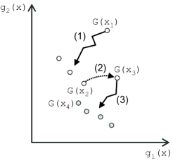
Figure 1: Illustration of the Pareto Iterated Local Search metaheuristic. The archive of the currently best solutions is updated during the search. Here, $G(x_{4})$ dominates $G(x_{2})$ which is going to be deleted from $P^{approx}$.

The PILS metaheuristic may be formalized as given in Algorithm 1. The intensification of the algorithm, illustrated in the steps (1) and (3) of Figure 1 is within the lines 6 to 21, the description of the diversification, given in step (2) of Figure 1 is within the lines 22 to 26.

Algorithm 1 Pareto Iterated Local Search

1:  Initialize control parameters: Define the neighborhoods $\mathbf{N}_{1},\ldots,\mathbf{N}_{k}$

2:  Set $i=1$

3:  Generate initial solution $x$

4:  Set $P^{approx}=\{x\}$

5:  repeat

6:     repeat

7:        Compute $\mathbf{N}_{i}(x)$

8:        Evaluate $\mathbf{N}_{i}(x)$

9:        Update $P^{approx}$ with $\mathbf{N}_{i}(x)$

10:        if $\exists x^{\prime}\in\mathbf{N}_{i}(x)\mid x^{\prime}\preceq x$ then

11:           Set $x=x^{\prime}$

12:           Set $i=1$

13:           Rearrange the neighborhoods $\mathbf{N}_{1},\ldots,\mathbf{N}_{k}$ in some random order

14:        else

15:           Set $i=i+1$

16:        end if

17:     until $x$ locally optimal with respect to $\mathbf{N}_{1},\ldots,\mathbf{N}_{k}$, therefore $i>k$

18:     Set neighborhoods of $x$ as ‘investigated’

19:     Set $i=1$

20:     if $\exists x^{\prime}\in P^{approx}\mid$ neighborhoods not investigated yet then

21:        Set $x=x^{\prime}$

22:     else

23:        Select $x^{\prime}\in P^{approx}$

24:        Compute $x^{\prime\prime}=\mathbf{N}_{perturb}(x^{\prime})$

25:        Set $x=x^{\prime\prime}$

26:     end if

27:  until termination criterion is met

It can be seen, that the algorithm computes a set of neighborhoods for each alternative. The sequence in which the neighborhoods are computed is arranged in a random fashion, described in line 13 of Algorithm 1. This introduces an additional element of diversity to the concept, as otherwise the search might be biased by a certain sequence of neighborhoods.

4 An Application to Multi-Objective Flow Shop Scheduling

4.1 Configuration of the Algorithm and Experimental Setup

In the following, the Pareto Iterated Local Search is applied to a set of benchmark instances of the multi-objective permutation flow shop scheduling problem. They have been provided by (Basseur, Seynhaeve and Talbi, 2002), who first defined due dates for the well-known instances of (Taillard, 1993). The instances range from $n=20$ jobs that have to be processed on $m=5$ machines to $n=100,m=20$. All of them are solved under the simultaneous consideration of the minimization of the maximum completion time $C_{max}$ and the total tardiness $T_{sum}$.

Three operators are used in the definition of the neighborhoods $\mathbf{N}_{1},\ldots,\mathbf{N}_{k}$, described in the work of (Reeves, 1999). First, an exchange neighborhood, exchanging the position of two jobs in $\pi$, second, a forward shift neighborhood, taking a job from position $i$ and reinserting it at position $j$ with $j<i$, and finally a backward shift neighborhood, shifting a job from position $i$ to $j$ with $j<i$. All operators are problem independent, each computing $\frac{n(n-1)}{2}$ neighboring solutions.

After a first approximation $P^{approx}$ of the Pareto set is obtained, one element $x^{\prime}\ P^{approx}$ is selected by random and perturbed into another solution $x^{\prime\prime}$. We use a special neighborhood that on one hand leaves most of the characteristics of the perturbed alternatives intact, while still changes the positions of some jobs. Also, several consecutive applications of the neighborhoods $\mathbf{N}_{1},\ldots,\mathbf{N}_{k}$ are needed to return from $x^{\prime\prime}$ back to $x^{\prime}$. This is important, als otherwise the algorithm might navigate straight back to the initially perturbed alternative, possibly leading to a cycle in the search path.
The perturbation neighborhood $\mathbf{N}_{perturb}$ can be described as follows. First, a subset of $\pi$ is randomly selected, comprising four consecutive jobs at positions $j,j+1,j+2,j+3$. Then a neighboring solution is generated by moving the job at position $j$ to $j+3$, the one at position $j+1$ to $j+2$, the one at position $j+3$ to $j$, and the job at position $j+3$ to $j+2$. In brief, this leads to a combination of several exchange and shift moves, executed at once.

The benchmark instances of Basseur have been solved using the PILS algorithm. In each of the 100 test runs, the approximation quality of the obtained results has been analyzed using the $D_{1}$ and $D_{2}$ metrics of (Czyżak and Jaszkiewicz, 1998). While for the smaller instances the optimal solutions are known, the analysis for the larger instances has to rely on the best known results published in the literature. Experiments have been carried out on a Intel Pentium IV processor, running at 1.8 GHz. Table 1 gives an overview about the number of evaluations executed for each instance. Clearly, considerable more alternatives have to be evaluated with increasing size of the problem instances to allow a convergence of the algorithm.

Table 1: Number of evaluations for each investigated instance

Instance $n\times m$	No of evaluations
$20\times 5$ (#1)	1,000,000
$20\times 5$ (#2)	1,000,000
$20\times 10$ (#1)	1,000,000
$20\times 10$ (#2)	1,000,000
$20\times 20$	1,000,000
$50\times 5$	5,000,000
$50\times 10$	5,000,000
$50\times 20$	5,000,000
$100\times 10$	10,000,000
$100\times 20$	10,000,000

An implementation of the algorithm has been made available within the MOOPPS computer system, a software for the resolution of multi-objective scheduling problems using metaheuristics. The system is equipped with an extensive user interface that allows an interaction with a decision maker and is able to visualize the obtained results in alternative and outcome space. The system also allows the comparison of results obtained by different metaheuristics. For a first analysis, we compare the results obtained by PILS to the approximations of a multi-objective multi-operator search algorithm MOS, described in Algorithm 2.

Algorithm 2 Multi-objective multi-operator search algorithm

1:  Generate initial solution $x$, set $P^{approx}=\{x\}$

2:  repeat

3:     Randomly select some $x\in P^{approx}\mid$ neighborhoods not investigated yet

4:     Randomly select some neighborhood $\mathbf{N}_{i}$ from $\mathbf{N}_{1},\ldots,\mathbf{N}_{k}$

5:     Generate $\mathbf{N}_{i}(x)$

6:     Update $P^{approx}$ with $\mathbf{N}_{i}(x)$

7:     if $x\in P^{approx}$ then

8:        Set neighborhoods of $x$ as ‘investigated’

9:     end if

10:  until $\not\!\exists x\in P^{approx}\mid$ neighborhoods not investigated yet

The MOS Algorithm is based on the concept of Variable Neighborhood Search, extending the general idea of several neighborhood operators by adding an archive $P^{approx}$ towards the optimization of multi-objective problems. For a fair comparison, the same neighborhood operators are used as in the PILS algorithm. After the termination criterion is met in step 10, we restart search while keeping the approximation $P^{approx}$ for the final analysis of the quality of the obtained solutions.

4.2 Results

The average values obtained by the investigated metaheuristics are given in Table 2. It can be seen, that PILS leads for all investigated problem instances to better results for both the D₁ and the $D_{2}$ metric. This general result is consistent independent from the actual problem instance. For a single instance, the $20\times 5$ (#1), PILS was able to identify all optimal solutions in all test runs, leading to average values of $D_{1}=D_{2}=0.0000$. Apparently, this instance is comparably easy to solve.

Table 2: Average results of $D_{1}$ and $D_{2}$

	$D_{1}$		$D_{2}$
Instance $n\times m$	PILS	MOS	PILS	MOS
$20\times 5$ (#1)	0.0000	0.0323	0.0000	0.1258
$20\times 5$ (#2)	0.1106	0.1372	0.3667	0.4249
$20\times 10$ (#1)	0.0016	0.0199	0.0146	0.0598
$20\times 10$ (#2)	0.0011	0.0254	0.0145	0.1078
$20\times 20$	0.0088	0.0286	0.0400	0.1215
$50\times 5$	0.0069	0.0622	0.0204	0.1119
$50\times 10$	0.0227	0.3171	0.0897	0.4658
$50\times 20$	0.0191	0.3966	0.0616	0.5609
$100\times 10$	0.0698	0.3190	0.1546	0.4183
$100\times 20$	0.0013	0.2349	0.0255	0.3814

A deeper analysis has been performed to monitor the resolution behavior of the local search algorithms and to get a better understanding of how the algorithm converges towards the Pareto front. Figure 2 plots with $\times$ the results obtained by random sampling 50,000 alternatives for the problem instance $100\times 10$, and compares the points obtained during the first intensification procedure of PILS until a locally optimal set is identified. The alternatives computed starting from a random initial solution towards the Pareto front are plotted as $+$, the Pareto front as $\odot$. It can be seen, that in comparison to the initial solution even a simple local search approach converges in rather close proximity to the Pareto front. With increasing number of computations however, the steps towards the optimal solutions get increasingly smaller, as it can be seen when monitoring the distances between the $+$ symbols. After convergence towards a locally optimal set, overcoming local optimality is then provided by means of the perturbation neighborhood $\mathbf{N}_{perturb}$.

Figure 2: Randomly generated solutions ($\times$), intensification of search($+$), and Pareto front ($\odot$)

An interesting picture is obtained when analyzing the distribution of the randomly sampled 50,000 alternatives for instance $100\times 10$. In Figure 3, the number of alternatives with a certain combination of objective function values are plotted and compared to the Pareto front, given in the left corner. It turns out that many alternatives are concentrated around some value combination in the area of approximately $C_{max}=6900$, $T_{sum}=111500$, relatively far away from the Pareto front.

Figure 3: Distribution of randomly generated solutions ($+$) compared to the Pareto front $\odot$)

When analyzing the convergence of local search heuristics toward the globally Pareto front as well as towards locally optimal alternatives, the question arises how many local search steps are necessary until a locally optimal alternative is identified. From a different point of view, this problem is discussed in the context of computational complexity of local search (Johnson, Papadimitriou and Yannakakis, 1988). It might be worth investigating this behavior in quantitative terms. Table 3 gives the average number of evaluations that have been necessary to reach a locally optimal alternative from some randomly generated initial solution. The analysis reveals that the computational effort grows exponentially with the number of jobs $n$.

Table 3: Number of evaluations until a locally optimal alternative is reached

Instance $n\times m$	No of jobs	No of evaluations
$20\times 5$ (#1)	20	3.614
$20\times 5$ (#2)	20	3.292
$20\times 10$ (#1)	20	2.548
$20\times 10$ (#2)	20	2.467
$20\times 20$	20	2.657
$50\times 5$	50	53.645
$50\times 10$	50	55.647
$50\times 20$	50	38.391
$100\times 10$	100	793.968
$100\times 20$	100	479.420

5 Conclusions

In the past years, considerable progress has been made in the resolution of complex multi-objective optimization problems. Effective metaheuristics have been developed, providing the possibility of computing approximations to problems with numerous objectives and complex side constraints. While many approaches are of increasingly effectiveness, complex parameter settings are however required to tune the solution approach to the given problem at hand.

The algorithm presented in this paper proposed a metaheuristic, combining two recent principles of local search, Variable Neighborhood Search and Iterated Local Search. The main motivation behind the concept is the easy yet effective resolution of multi-objective optimization problems with an approach using only few parameters.

After an initial introduction to the problem domain of flow shop scheduling under multiple objectives, the introduced PILS algorithm has been applied to a set of scheduling benchmark instances taken from literature. We have been able to obtain encouraging results, despite the simplicity of the algorithmic approach. A comparison of the approximations of the Pareto sets has been given with a multi-operator local search approach, and as a conclusion PILS was able to lead to consistently better results.
The presented approach seems to be a promising tool for the effective resolution of multi-objective optimization problems. After first tests on problems from the domain of scheduling, the resolution behavior on problems from other areas might be an interesting direction for further developments.

6 References

Bagchi, T.P. (1999), Multiobjective scheduling by genetic algorithms, Boston, Dordrecht, London: Kluwer Academic Publishers.

Bagchi, T.P. (2001), “Pareto-optimal solutions for multi-objective production scheduling problems”, in Zitzler, E., Deb, K., Thiele, L., Coello Coello, C.A. and Corne, D., editors, Evolutionary Multi-Criterion Optimization: Proceedings of the First International Conference EMO 2001, Berlin, Heidelberg, New York: Springer Verlag, 458–471.

Baker, K.R. (1974), Introduction to Sequencing and Scheduling, New York, London, Sydney, Toronto: John Wiley & Sons.

Basseur, M., Seynhaeve, F. and Talbi, E. (2002), “Design of multi-objective evolutionary algorithms: Application to the flow-shop scheduling problem”, in Congress on Evolutionary Computation (CEC’2002), Piscataway, NJ: IEEE Service Center, 1151–1156.

Błażewicz, J., Ecker, K.H., Pesch, E., Schmidt, G. and Wȩglarz, J. (2001), Scheduling Computer and Manufacturing Processes, Berlin, Heidelberg, New York: Springer Verlag.

Czyżak, P. and Jaszkiewicz, A. (1998), “Pareto simulated annealing - a metaheuristic technique for multiple-objective combinatorial optimization”, Journal of Multi-Criteria Decision Analysis, 7, 34–47.

Glover F. and Kochenberger, G.A. (2003), Handbook of Metaheuristics, volume 57 of International Series in Operations Research & Management Science, Boston, Dordrecht, London: Kluwer Academic Publishers.

Hansen, P. and Mladenović, N. (2003), “Variable neighborhood search”, in Glover, F. and Kochenberger, G.A. (2003), chapter 6, 145–184.

Ishibuchi, H. and Murata, T. (1998), “A multi-objective genetic local search algorithm and its application to flowshop scheduling”, IEEE Transactions on Systems, Man, and Cybernetics, 28, 392–403.

Johnson, D.S., Papadimitriou C.H. and Yannakakis, M. (1988), “How Easy Is Local Search?”, Journal of Computer and System Sciences, 37, 79–100.

Loukil, T., Teghem, J. and Tuyttens, D. (2005), “Solving multi-objective production scheduling problems using metaheuristics”, European Journal of Operational Research, 161, 42–61.

Lourenço, H.R., Martin, O. and Stützle, T. (2003), “Iterated local search”, in Glover, F. and Kochenberger, G.A. (2003), chapter 11, 321–353.

Murata, T., Ishibuchi, H. and Tanaka, H. (1996), “Multi-objective genetic algorithm and its application to flowshop scheduling”, Computers & Industrial Engineering, 30, 957–968.

Nagar, A., Heragu, S.S. and Haddock, J. (1996), “A combined branch-and-bound and genetic algorithm based approach for a flowshop scheduling problem”, Annals of Operations Research, 63, 397–414.

Pinedo, M. (2002), Scheduling: Theory, Algorithms, and Systems, Upper Saddle River, NJ: Precentice Hall.

Reeves, C.R. (1999), “Landscapes, operators and heuristic search”, Annals of Operations Research, 86, 473–490.

Taillard, E. (1993), “Benchmarks for basic scheduling problems”, European Journal of Operational Research, 64, 278–285.

T’kindt, V. and Billaut, J.-C. (2002), Multicriteria Scheduling: Theory, Models and Algorithms, Berlin, Heidelberg, New York: Springer Verlag.

Ulungu, E.L., Teghem, J., Fortemps, P.H. and Tuyttens, D. (1999), “MOSA method: A tool for solving multiobjective combinatorial optimization problems”, Journal of Multi-Criteria Decision Making, 8, 221–236.

Vincke, P. (1992), Multicriteria Decision-Aid, Chichester, New York, Brisbane, Toronto, Singapore: John Wiley & Sons.