CME liftoff with high-frequency fragmented type II burst emission

Abstract

Aims.

Methods.

Results.

Abstract

Aims. Solar radio type II bursts are rarely seen at frequencies higher than a few hundred MHz. Since metric type II bursts are thought to be signatures of propagating shock waves, it is of interest to know how these shocks, and the type II bursts, are formed. In particular, how are high-frequency, fragmented type II bursts created? Are there differences in shock acceleration or in the surrounding medium that could explain the differences to the “typical” metric type IIs?

Methods. We analyse one unusual metric type II event in detail, with comparison to white-light, EUV, and X-ray observations. As the radio event was associated with a flare and a coronal mass ejection (CME), we investigate their connection. We then utilize numerical MHD simulations to study the shock structure induced by an erupting CME in a model corona including dense loops.

Results. Our simulations show that the fragmented part of the type II burst can be formed when a coronal shock driven by a mass ejection passes through a system of dense loops overlying the active region. To produce fragmented emission, the conditions for plasma emission have to be more favourable inside the loop than in the interloop area. The obvious hypothesis, consistent with our simulation model, is that the shock strength decreases significantly in the space between the denser loops. The later, more typical type II burst appears when the shock exits the dense loop system and finally, outside the active region, the type II burst dies out when the changing geometry no longer favours the electron shock-acceleration.

1 Introduction

Radio type II bursts are observed in association with flares and coronal mass ejections (CMEs). These bursts can be observed at metric wavelengths (coronal type II bursts) and at decameter and longer wavelengths (interplanetary type II bursts). The mechanism behind the bursts is generally assumed to be a propagating shock which creates electron beams that excite Langmuir waves, which in turn convert into radio waves at the local plasma frequency and its second harmonic (Melrose, 1980; Cairns et al., 2003). As shocks can be formed in various ways (for an overview see, e.g., Warmuth, 2007; for the terminology see, e.g., Vrs̆nak, 2005), it is not evident that all solar radio type II bursts are formed in the same way.

Most of the interplanetary type II bursts are thought to be created by CME-driven shocks, but there is observational evidence that at least some coronal metric type II bursts are ignited by smaller-scale processes associated with the flare energy release, such as high-speed plasma jets/blobs or loop ejections/expansions (Klein et al., 1999; Pohjolainen et al., 2001; Khan & Aurass, 2002; Klassen et al., 2003; Dauphin et al., 2006; Pohjolainen, 2008). Statistically, there is support for the idea that metric type II bursts have their root cause in fast coronal mass ejections (Cliver et al., 1999), but also that they are not caused by shocks driven in front of CMEs (Cane & Erickson, 2005).

Metric type II bursts can be observed in dynamic radio spectra as slowly (0.1 – 1.0 MHz s^-1) drifting emission lanes (Nelson & Melrose, 1985)). The start frequency of metric type II bursts is usually at about 100 – 200 MHz, and the bursts have a typical duration of 2 – 18 min (Subramanian & Ebenezer, 2006). In some cases it is possible to separate a slowly drifting “backbone” in the burst emission, with fast-drifting ($\sim$ 10 MHz s^-1) emission stripes shooting up and down from the backbone (Mann & Klassen, 2005). These features have been named as “herringbones”, and they bear some resemblance to radio type III bursts which are signatures of outflowing electron beams. However, the drift rates of type III bursts have been found to be higher than those of herringbones (Mann & Klassen, 2002).

In this paper, we analyse in detail one metric type II burst that occurred on 13 May 2001. The burst started at an unusually high frequency, proceeded showing fragmented and curved emission bands, which were visible at the fundamental and second harmonic plasma frequencies. As the radio burst was associated with a flare and a CME, we do a multi-wavelength analysis in order to identify the origin of the shock that formed the radio type II burst. We then use numerical MHD simulations to verify the results from the data analysis.

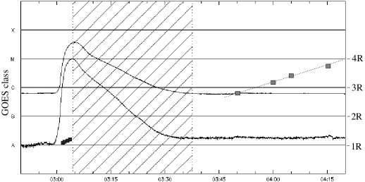
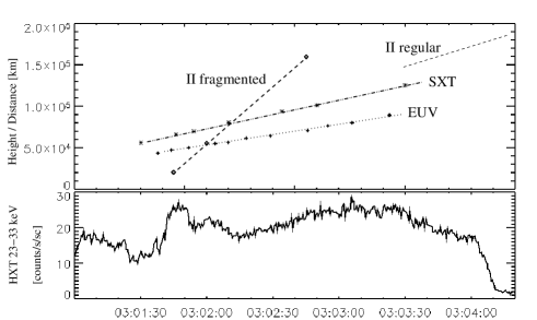
Figure 1: Left: GOES soft X-ray flux curve at 02:50 – 04:20 UT, with flare class classification A–X. The dashed region indicates Yohkoh satellite night time, when no observations are available from the experiment. Plane-of-the-sky heliocentric CME front distances (boxes combined with a dotted line) are from the LASCO CME Catalog. Black boxes between 03:01:30 and 03:03:30 UT show the projected distances of the soft X-ray loop-like front, measured from the center of the eruption region at 1 R_⊙. Right: Detailed plot of the estimated distances/heights measured in the time interval 03:01:00 – 03:04:20 UT. Projected distances (km) from the eruption center are shown for the SXT loop-like front (stars/dash-dotted line) and the EUV ’blob’ (crosses/dotted line). The estimated type II burst heights are calculated with the 10$\times$Saito density model for the fragmented part (the three height–time data points, marked with diamonds, are from the start times of each three fragment. The type II heights for the later regular part (dashed lines) are calculated with the hybrid density model (corresponding to 5$\times$Saito) which describes a “standard” solar atmosphere. Applying a high-density model like 10$\times$Saito for the regular type II part at $\lesssim$ 130 MHz would imply at least streamer densities, see text for details. Yohkoh HXT hard X-ray counts in the 23 – 33 keV energy channel are also shown (bottom panel). Note that the drop in counts near 03:04 UT is due to the satellite entering night time.

2 Observations

A GOES M3.6 class flare was observed to start at 02:58 UT on 13 May 2001 in NOAA AR 9455 (S18 W01). The flare maximum occurred at 03:04 UT, and at 03:50 UT a coronal mass ejection was detected in the LASCO (Brueckner et al., 1995) C2 images. The CME front moved toward the South at a speed of 430 km s^-1 (LASCO CME Catalog, both the linear and second-order fits to the height–time data give similar speeds). Backward-extrapolation of the heights indicates a CME start time near 03:00 UT. Fig. 1 shows the GOES soft X-ray flux curve, with the CME plane-of-the-sky heights during 02:50 – 04:20 UT. Yohkoh HXT (Kosugi et al., 1991) hard X-ray counts are shown at 03:01:00 – 03:04:20 UT, before satellite night ended the observations.

Radio emission at decimetric–metric wavelengths was observed to start at 03:01:45 UT. It consisted of a type II burst that was clearly visible as two emission lanes, starting near 500 and 1000 MHz. It was followed by bursty continuum emission at 700 – 300 MHz. These features are shown in the HiRAS dynamic spectrum that covers a wide, 2500–25 MHz frequency range, in Fig. 2. The type II burst emission ended abruptly at 03:05:15 UT near 90 MHz at the fundamental emission band (visible also in the RSTN observations at 180–25 MHz). No interplanetary type II emission was observed at lower frequencies, as verified from the Wind WAVES (Bougeret et al., 1995) observations at 14 MHz–20 kHz.

2.1 Fragmented radio type II burst

The radio type II burst showed a pair of fundamental and second harmonic emissions, which clearly marks it as plasma emission,

$$f_{p}=9000\sqrt{n_{e}},$$ (1)

where the local electron plasma frequency $f_{p}$ is expressed in Hz and the electron density $n_{e}$ in cm^-3. As plasma emission at the fundamental is directly related to the local electron density, we can use the spectral observations to calculate electron densities and to estimate burst source heights and speeds. Height estimates require, however, the use of atmospheric density models, which are not unambiguous, see e.g., Vrs̆nak et al. (2004a) and Pohjolainen et al. (2007).

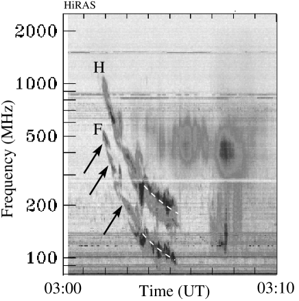
Figure 2: HiRAS dynamic spectrum from the 25-2500 MHz frequency range, at 03:00–03:10 UT on 13 May 2001. ’F’ notes emission at the fundamental and ’H’ at the second harmonic plasma frequency. Arrows point to the fragmented emission bands and dashed white lines outline the later-appearing “regular” type II burst lanes.

The 500 MHz start frequency (fundamental plasma emission) is unusually high for a type II burst (Lin et al., 2006). During the first two minutes of the burst, the emission was fragmented into separate, curved emission bands. The frequency drifts (fundamental emission) within the fragments were between 1.8 and 4.3 MHz s^-1. These drift rates are high compared to type II bursts in general, but consistent with drift rates found for high-frequency type II bursts, see Fig. 2a in Vrs̆nak et al. (2002). The first “fragment” showed emission between 500 and 420 MHz, which correspond to densities in the range of 2 – 3 $\times$ 10⁹ cm^-3. The second fragment near 03:02 UT gives densities 1 – 2 $\times$ 10⁹ cm^-3 (400 – 310 MHz), and the third near 03:03 UT gives densities 2 – 6 $\times$ 10⁸ cm^-3 (220 – 130 MHz). These values indicate that the source regions were dense, similar to active region loops. Rough estimates for heliocentric heights, using atmospheric density models up to ten-times Saito (Saito, 1970), give values in the range of 1.03 – 1.43 R_⊙. These estimates are suggestive, since the models do not give heights for erupting structures. The calculated type II burst source heights (10$\times$Saito densities) are shown at the start times of the three fragmented emission bands in Fig. 1. The burst velocity, using these heights, is as high as 2 300 km s^-1, which probably reflects the gradual density gradient in the Saito density model. For comparison, if we calculate the burst speed from a steeper density gradient, using the emission frequency (500 MHz) and the general drift-rate of the bands (2.4 MHz s^-1), and the scale height of 73 000 km (hydrostatic isothermal scale height at 1.25 MK coronal temperature and heliocentric height of 1.1 R_⊙), we get a burst speed of $\approx$ 1 000 km s^-1 (for the method see, e.g., Pohjolainen et al., 2007).

At 03:03:35 UT the type II lanes got wider and started to look like a typical type II burst. The start frequency of this “regular” part was 130 MHz at the fundamental, and the frequency drift was about 0.4 MHz s^-1. This is within the usual drift rates observed for type II bursts (between 0.1 and 1.0 MHz s^-1). To estimate the height for this part of the type II burst we use the hybrid density model by Vrs̆nak et al. (2004a). This model gives density values similar to five-times Saito in the low corona but also links coronal densities to those in the interplanetary space. The heliocentric heights for the burst source are 1.22 R_⊙ at the beginning of the burst (130 MHz), and 1.34 R_⊙ at the end of the burst at 03:05:15 UT (90 MHz). A height–time trajectory for this regular type II burst part is also shown in Fig. 1. Applying a high-density model like 10$\times$Saito also for the regular type II part would make the two type II burst tracks converge, but this would imply that the regular part was formed at least at streamer densities, above 1.4 R_⊙. If the burst source was moving along the density gradient the deduced speed from the hybrid model is approximately 840 km s^-1. If the direction of motion differed from that, the speed could have been higher (an angle of 45^∘ between the driver velocity vector and the density gradient produces a speed 1.4 times higher).

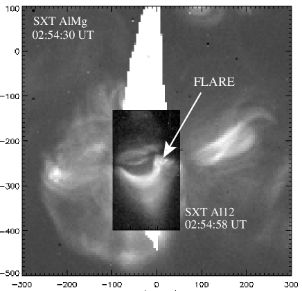
Figure 3: Yohkoh SXT composite of images taken with two different filters and field of views at 02:54 UT on 13 May 2001. It shows the pre-eruption flare region and interconnecting loops. Axes are in arc seconds and white areas in the image mark saturated pixels.

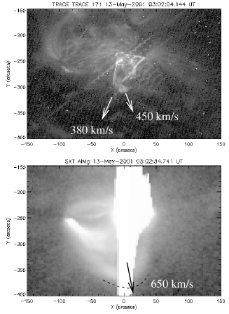
Figure 4: TRACE EUV image at 03:02:04 UT (top), showing the erupting filament. Most of the filament material moved toward the Southeast (speed $\approx$ 380 km s^-1), but a blob-like structure moved more to the Southwest (speed $\approx$ 450 km s^-1). Arrows give the direction of motion for these structures. Yohkoh SXT image (bottom) shows the same region in soft X-rays. The pointing for TRACE seems to be off from that of Yohkoh and so point-to point comparison is ambiguous.

2.2 Eruptive flare

The pre-eruption Yohkoh SXT (Tsuneta et al., 1991) images show several loop systems, connected both to the active region and regions nearby (Fig. 3). Small-scale pre-flare brightenings were observed before the flare start at 02:58 UT. The flare region is indicated with an arrow in Fig. 3.

EUV images taken with TRACE (Handy et al., 1999) show a filament eruption, in which most of the material is moving toward the Southeast. The outermost front of the filament moves with a projected speed of about 380 km s^-1, but there is also a separate ’blob’ that moves more to the Southwest with a projected speed of 450 km s^-1, see Fig. 4. The TRACE image in Fig. 4 is at 03:02:04 UT, very near the time when the first fragmented radio type II burst band appeared.

Yohkoh SXT observed the flare until 03:04 UT, when satellite night set in. The partial SXT frames between 03:02 and 03:03 UT reveal a loop-like front moving Southward at a projected speed of about 650 km s^-1, see Figs. 4 and 5. The projected distances for the SXT loop-like front and the EUV blob, calculated from the eruption center where loop footpoints were visible prior to the event, are shown in Fig. 1, together with the type II burst height estimates (at 10$\times$Saito atmospheric densities). The height of the first type II burst fragment is low compared to the SXT and EUV structure heights, but there is also some uncertainty in the true density gradient. The fragment heights, if true, suggest that the shock may have travelled through the EUV and/or soft X-ray structures. On the other hand, a low type II start height also suggests that the type II burst may have been emitted at the low-lying flanks of the shock. If, however, the speed of the propagating shock remained in the range of 1 000 – 850 km s^-1 during the whole event, the fragmented burst could have started at heliocentric height of 1.1 R_⊙ ($\approx$ 70 000 km above the photosphere), which is just above the SXT loop-like front.

As Yohkoh SXT was observing with two different filters, Be and AlMg, it is possible to estimate the emission measure $EM$ using the filter ratio, see, e.g., McTiernan et al. (1993). The emission measure for the outermost SXT loop-like structure at 03:02:18 UT is 6 $\times$ 10⁴³ – 10⁴⁴ cm^-3 per pixel. As one pixel is 2.5″and the loop width is approximately 10″in the images, we can estimate the loop depth along the line of sight to be equal to the loop width, $\approx$ 4 pixels, and thus get an emitting volume $V$ of 2.3 $\times$ 10²⁵ cm³ per pixel. Assuming an isothermal homogeneous source, the electron density $N$ can be calculated from $N\approx\sqrt{EM/V}$, which gives a value of about 1.6 – 2.1 $\times$ 10⁹ cm^-3. For comparison, the fragmented radio emission near 03:02 UT indicated electron densities of 1 – 2 $\times$ 10⁹ cm^-3, a value similar to our soft X-ray loop densities.

The SXT difference image at 03:03:30 – 03:02:50 UT (Fig. 5) shows that the (projected) soft X-ray loop-like front was located approximately 180″ from the center of the flaring region. This corresponds roughly to a distance of 126 000 km. For comparison, the estimated height of the later, regular part of the type II burst source at 03:03:35 UT is about 152 000 km. Even taking into account projection effects, the radio burst source is located higher than the soft X-ray loop-like front at that time.

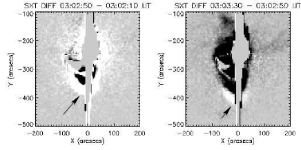
Figure 5: SXT difference images (AlMg filters) at 03:02:50 UT and 03:03:30 UT, showing the loop-like eruption front in soft X-rays. The later difference image is near the time of the appearance of the ’regular’ metric type II burst at 03:03:35 UT. The projected plane-of-the sky speed of the soft X-ray front is about 650 km s^-1 (arrows point to the loop front).

3 Coronal conditions

If we assume a structure moving through a system of dense loops at a speed of 850 km s^-1 (similar to the inferred metric type II shock speed; see also Sect. 5), shock-acceleration could be created if the speed of the disturbance exceeded the local magnetosonic speed. In the solar corona, the local Alfvén speed $v_{A}$ is a good approximation for the magnetosonic speed,

$$v_{A}\approx\frac{2\times 10^{11}B}{\sqrt{n_{e}}},$$ (2)

where $B$ is the magnetic field strength and $n_{e}$ is the local electron density, in gaussian units. In order to make the disturbance velocity super-Alfvénic at the density of the first type II fragment (2 - 3 $\times$ 10⁹ cm^-3), the magnetic field strength should be less than 22 G. At the time of the third fragment, the electron density was 2 - 6 $\times$ 10⁸ cm^-3, implying a field strength less than 10 G. The empirical scaling law presented by Dulk & McLean (1978) gives the strength of the coronal magnetic field above active regions as $B$ = 0.5 $\times$ $h^{-1.5}$ G, where $h$ is the height above the photosphere expressed in solar radiae. Field strengths of 22 G would then appear at about heights of 56 000 km and 10 G at about 95 000 km. The outermost SXT loop heights, approximated from the observed projected distances between the loop footpoints and the loop fronts, were about 66 000 km at the time of the first type II fragment and about 100 000 km at the time of the third fragment. The EUV blob was located lower, at about 47 000 and 71 000 km, respectively. The estimated field strengths imply that the shock could have been located at about the SXT loop heights at the time of the fragmented type II burst.

Basically, any propagating shock would be able to excite a type II burst, since the type II characteristics mainly reflect the medium where the shock is propagating. The SXT loop-like front could have been a low-coronal signature of the CME (Rust & Hildner, 1976; Vrs̆nak et al., 2004b; Temmer et al., 2008), which drives the shock. The shock could also have been ignited by the flare, and propagated as a blast wave. In this scenario, if the SXT loop-like front roughly corresponds to the CME front, the type II fragmented emission would be excited at segments where the shock overtakes some part of the CME – and the type II fragments would be attributed to the inhomogeneities within the erupting structure. One difference between shock types is that a blast wave should weaken in time as it does not gain energy on the way, and because it also expands the energy is divided into a larger area. Eventually a blast wave shock will become so weak that it cannot accelerate electrons any more, leading to a slow fade out of the type II burst.

The type II burst disappearance from the spectrum was quite sudden at 03:05:15 UT. The abrupt end suggests that the shock may not have been weakening but instead it entered a region where the magnetic field orientation was very different, e.g., there was a transit from a perpendicular to a parallel shock region. Shock-drift acceleration is very efficient for quasi-perpendicular shocks, and a change in the geometry could stop accelerating particles. Of course, this could happen both to a driven shock and a freely propagating blast wave shock (before it weakens). In the case where a blast wave shock overtakes a CME, type II emission could end after the overtake (Gary et al., 1984).

4 MHD modeling

We utilize numerical simulations to study the shock structure induced by an erupting CME in a model corona including dense loops. Since we are interested in modeling the first minutes of the eruption, we consider a local model of the low corona. The time-dependent, ideal MHD equations augmented with gravity are solved in a two-dimensional Cartesian domain. The details of the model have been presented by Pomoell et al. (2008), who employed a largely similar model to study the waves excited by an erupting flux rope.

The magnetic field configuration consists of a flux rope and an arcade-like background field. The field of the detached flux rope is created by a line current of radius $r_{0}$ situated at distance $h$ above the solar surface, and the arcade structure of the background structure follows the coronal arcade model of Oliver et al. (1993). While the density of the ambient corona decreases exponentially due to the choice of constant gravitational acceleration, $g_{\odot}=2.74\times 10^{4}$ cm s^-2, and constant initial temperature $T_{0}$ = 1.5 $\times$ 10⁶ K, the density inside the flux rope is enhanced to model denser filament material.

To include coronal loops with an increased density into the model, we apply a simple approach in which the magnetic field strength is decreased in the denser loops so that the total pressure is constant at a constant height. For the details of this procedure, we refer to the work of Odstrc̆il & Karlický (2000). Note that in real coronal loops, both the magnetic field strength and density are enhanced compared with the ambient corona. We discuss in section 6 the implications of this when comparing the results of the simulations with the observations.

Table 1: Alfvén speed in km/s at four locations $(x,y)$ for the two initial conditions

Run	$(-0.16,1)$	$(0,1.1)$	$(0,1.2)$	$(0,1.45)$
A	335	515	220	571
B & C	457	703	30	779

Fig. 6 shows the initial distribution of the density and Alfvén speed $\nu_{A}$ (isothermal sound speed) with some field lines of the magnetic field superimposed. Table 1 gives the Alfvén speed at four locations for the two initial conditions considered (see section 5). Note that $\nu_{A}$ increases as a function of height (away from the fluxrope), but varies less inside the loop.

             Density            Alfvén speed         $\rho$        $\nu_{A}$

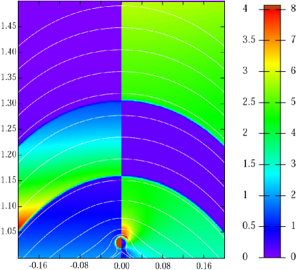
$y$

                          $x$

Figure 6: The initial state of the simulation: density (left half) and Alfvén speed (right half). The white lines depict magnetic field lines. The units in the color bar are for the density (left values in the color bar) $1.67\times 10^{-15}\mbox{ g\,cm}^{-3}$ and for the Alfvén speed (right values in the color bar) $143\mbox{ km\,s}^{-1}$, the isothermal sound speed. Note the clipping of the color bar; a brown color indicates values larger than the color bar maximum.

                 Density            Speed              $\rho$,$\nu$

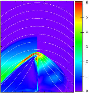
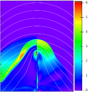
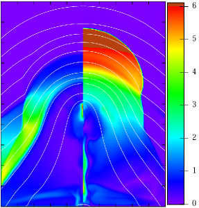
  (a)

  (b)

  (c)

Figure 7: The density (left half) and speed (right half) at three different times, $t=220$ (a), $t=270$ (b) and $t=330$ (c) seconds. The white lines depict the magnetic field lines. The units in the color bar are for the density $1.67\times 10^{-15}\mbox{ g\,cm}^{-3}$ and for the speed $143\mbox{ km\,s}^{-1}$. Note that both quantities are plotted using the same color bar.

The flux rope is made to erupt by invoking an artificial force that acts on the flux rope plasma elements during the simulation, similar to the study of Pomoell et al. (2008). The Cartesian grid of the simulation consists of $300\times 300$ cells in the $x\times y=[$-0.2 R_⊙, 0.2 R${}_{\odot}]\times[$1.0 R_⊙, 1.5 R${}_{\odot}]$ simulation domain. The boundary values are kept fixed during the simulation.

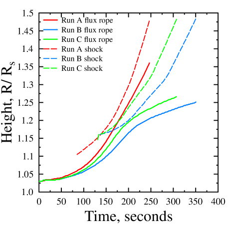
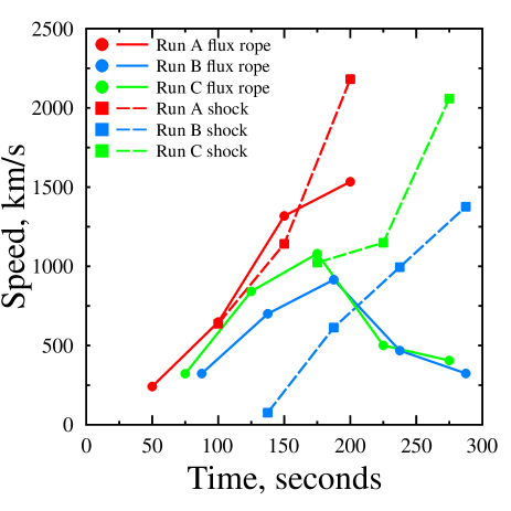
Figure 8: Left: Plot of the height-time data of the flux rope (solid line) and shock front (broken line) for the three simulation runs. Red corresponds to run A, green to run B and blue to run C. Right: Plot of the corresponding flux rope and shock speed.

5 Results of the simulations

Fig. 7 shows the mass density and speed at three different times, $t=220,270$ and $330$ seconds. The dynamics of the eruption is as follows: As the flux rope starts to rise, a perturbation is formed around the flux rope. Due to the gradient in the Alfvén speed and the increasing speed of the flux rope, the wave steepens to a shock ahead of the flux rope. However, the strength of the shock remains weak in the area below the loop. When the shock reaches the dense loop, it strengthens and slows down quickly due to the low Alfvén speed in the loop (panel a). The erupting filament continues to push the loop structure ahead of it, acting as the driver of the shock. Thus, the speed of the shock is roughly that of the displaced loop structure when propagating in the region of low $\nu_{A}$. As the filament decelerates, the displaced loop and shock escape from the filament (panel b). When reaching the region of higher $\nu_{A}$, the speed of the shock increases with the increasing $\nu_{A}$, and escapes from the propagating loop structure (panel c).

To quantify the description above, we plot in Fig. 8 the height-time profile of the filament and the shock. We consider three different runs with slightly different parameters. Run B (blue color coding) and C (green color coding) are identical but for the magnitude of the artificial accelerating force, which is larger for run C. Run A has the same magnitude of the accelerating force as run C, but the density contrast between the loop and ambient corona as well as the strength of the magnetic field is lower for run A. The speeds of the flux rope and shock are also shown in Fig. 8.

In all three cases, the shock is strong while it propagates in the loop, with the compression ratio remaining between 3 – 3.5. However, the behaviour after the shock exits the loop depends on the simulation run. For run A, the shock only slightly decreases in strength, while for runs B and C the compression ratio quickly decreases to approximately 2.2. Interestingly, the shock strength remains at this value until the end of the simulation.

In Fig. 9, we plot the radio emission produced by the shock assuming that the emission is produced immediately in front of the leading edge shock. The emission lane shows a frequency drop in accordance with the exponentially decreasing density. Additionally, we indicate the compression ratio of the shock by the size of the marker.

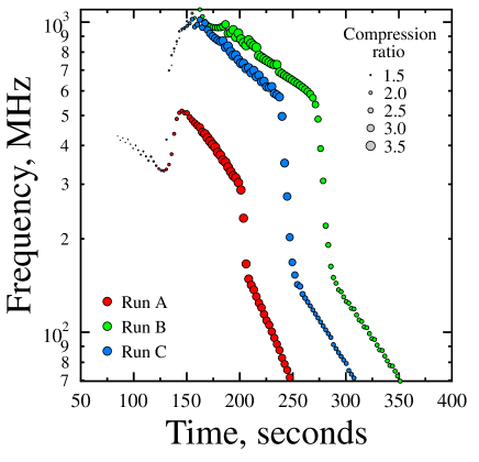
Figure 9: Radio track of the three simulation runs. The size of the marker indicates the compression ratio of the shock.

In addition to performing simulations with one dense loop, we also considered simulations with two loops. Adding another dense loop above the existing loop does not alter the overall dynamics of the eruption. However, the shock structure becomes very complex as the shock enters the second loop. We refrain from showing the results, but note that a similar plot as Fig. 9 in the two-loop case shows two distinct tracks, corresponding to the shock propagating in the dense loops. In between the loops the frequency drops significantly.

6 Discussion and conclusions

Observations on 13 May 2001 show that:

• The speed of the white-light, plane-of-the-sky CME (430 km s^-1) was similar to the projected speed of the erupting filament (380 km s^-1) and the EUV “blob” (450 km s^-1). The CME most probably consisted of the ejected filament, and the filament propagated in the wake of the soft X-ray loop-like front

• The projected speed of the soft X-ray loop-like front (650 km s^-1) and the estimated speed of the type II burst source ($>$ 850 km s^-1) were higher than the CME and EUV structure speeds

• The estimated soft X-ray loop densities agree with the plasma densities of the fragmented metric type II burst. Also magnetic field strengths are in agreement with a super-Alfvénic shock at speed $\approx$ 850 km s^-1 near the soft X-ray loop heights

• The fragmented type II burst changed appearance to a “regular” type II burst at a time when the propagating soft X-ray loop-like front approached the outer boundary of the active region

• The type II burst disappeared abruptly, without any weakening of the emission.

The MHD simulations that we have performed for a flux rope accelerated in a corona with dense loops show that:

• The CME eruption drives a shock wave ahead of it through the corona

• The shock wave propagates faster through the corona than its driver

• In the dense loops, the shock becomes significantly stronger

• Under right conditions, the shock strength decreases rapidly as the shock exits the loop.

It is consistent with the simulation model that the high speed of the loop-like soft X-ray front actually corresponds to a strong shock wave propagating through the loop. When outside the active region, the changing geometry no longer favours shock acceleration and the type II burst dies out. Together with the assumption that the shock wave generates conditions that produce type II bursts, our MHD model produces burst lanes that correspond qualitatively to those observed in the event. However, in order for the radio signature to become fragmented as is observed, the conditions for plasma emission have to be somehow more favourable inside the loop than in the interloop area. The obvious assumption, consistent with our simple simulation model, is that the shock strength decreases significantly in the space between the denser loops. This requires specific conditions, such as a very large difference in the Alfvén speed between the loop and interloop area, or a rapidly increasing Alfvén speed in the interloop area.

Our simplified two-dimensional model of coronal loops generates the favourable conditions for shock formation as it necessarily yields weak magnetic fields in the dense loops to achieve lateral pressure balance. This is obviously too restrictive an assumption, as real coronal loops involve both increased densities and magnetic fields. Thus, the strength of the shock in our model does not necessarily carry over to a more realistic model of the corona. However, the overlying coronal structure may actually be quite fragmented containing loops with different densities and magnetic fields, and our simulation model indicates that those with the lowest Alfvén speed produce the strongest shock. Note also that the strength of the shock is not the only factor affecting the radio emission from the shock. Other factors, such as the density of the electrons in the loop, are important for the plasma emission mechanism as well. Thus, the densest loops in the corona overlying the active region seem most probable sites of plasma emission.

It is also possible and even plausible that the three-dimensional structure of the corona plays a significant role. For instance, the different fragments of the bursts could originate from different loops that are not on top of each other. However, even in this case the interloop area must have specific conditions but not necessarily related to the strength of the shock, in order to cause the burst to suddenly stop emitting.

In conclusion, using results from multi-wavelength data analysis and numerical MHD simulations, we have established that the unusual metric type II radio burst on 13 May 2001 can be explained by a model, where a coronal shock driven by a mass ejection passes through a system of dense loops overlying the active region, where the ejection originates.