Properties of the scale factor measure

Abstract

We show that in expanding regions, the scale factor measure can be reformulated as a local measure: Observations are weighted by integrating their physical density along a geodesic that starts in the longest-lived metastable vacuum. This explains why some of its properties are similar to those of the causal diamond measure. In particular, both measures are free of Boltzmann brains, subject to nearly the same conditions on vacuum stability. However, the scale factor measure assigns a much smaller probability to the observed value of the cosmological constant. The probability decreases further, like the inverse sixth power of the primordial density contrast, if the latter is allowed to vary.

I Introduction

I.1 The measure problem

Like the cosmological constant problem Wei89 ; Pol06 ; TASI07 , the measure problem arises purely within the regime of validity of semi-classical gravity. All that is needed is a long-lived vacuum state GutWei83 , or a sufficiently flat scalar field potential Linde ; GonLin87 , with positive vacuum energy. Under these conditions, a finite spatial region will inflate eternally, generating an unbounded four-volume. All possible events will occur infinitely many times, and a cutoff is needed to compute probabilities.

Unlike the cosmological constant problem, the measure problem leaves a loophole: it is possible that the conditions for eternal inflation do not actually occur in Nature. But increasing evidence indicates otherwise.

Slow-roll inflation is the dominant paradigm explaining the origin of structure and the large-scale homogeneity and flatness of our universe. If we are prepared to believe that the moderately fine-tuned scalar field potential necessary for driving slow-roll inflation can arise in Nature, it is hard to imagine that the more generic feature of a local minimum cannot exist.

Moreover, the observed universe has positive vacuum energy Per98 ; Rie98 ; Dun08 . Unless our vacuum is unstable on a time scale of order ten billion years—which would require remarkable tuning—it alone suffices to generate eternal inflation.

Finally, the only extant explanation Sak84 ; Wei87 ; BP of the smallness of the observed dark energy—the cosmological constant problem—is the existence of a multidimensional landscape of metastable vacua in string theory. This is empirical evidence for string theory, and in particular for eternal inflation.

A theory of everything, if it gives rise to eternal inflation, should eventually allow us to derive a unique prescription for computing probability amplitudes from first principles. Yet our understanding of string theory, especially in cosmological settings, remains woefully incomplete. For now, a top-down solution to the measure problem seems elusive. Thus, we advocate following the traditional, phenomenological approach.

I.2 Phenomenological approach

Like any other theory, a compelling measure should be reasonably well-defined, simple, and general. In tackling a problem so vast and unfamiliar, it is natural to seek more specific guiding principles. For example, lessons from the black hole information paradox motivated the causal diamond measure Bou06 ; BouFre06a . We would be ill advised, however, to turn our intuition into dogma, insisting absolutely on theoretical properties that “any reasonable” measure “must” obey. Not only would we run the danger of putting in by hand the answers we wish to get; worse, our wishes may be misguided. Surely, for example, any reasonable measure must reward the volume expansion during slow-roll inflation in any given vacuum? In fact, this intuitive requirement invites conflict with experiment GarVil05 ; FelHal05 . The causal diamond measure abandoned volume-weighting, and the requirement seems now to have lost its dogmatic status DGSV08 ; Pag08 .

This brings us to the one property of a measure that we can insist on absolutely: that its experimental predictions not conflict with observations. In fact, many innocent-looking measures do conflict with observation, and violently so. Some conflicts are extremely robust, arising almost independently of the properties of the underlying vacuum landscape. Thus, they allow us to falsify measures even while we still have much to learn about the landscape.

For example, the proper time cutoff  Lin86a ; LinLin94 ; GarLin94 ; GarLin94a ; GarLin95 ; Lin06 predicts a very hot universe LinLin96 ; Gut00a ; Gut00b ; Gut04 ; Teg05 ; Lin07 ; Gut07 ; BouFre07 with probability 1 (the “Boltzmann babies” or youngness paradox). Measures that involve counting the number of observers per baryon Efs95 ; Vil95 ; Wei96 ; MarSha97 ; Vil04 ; GarSch05 ; Wei05 predict an empty, cold universe Pag06 ; BouFre06b with probability 1 (the “Boltzmann brain” paradox). Such paradoxes are important tools for testing and eliminating measure theories. We say “paradox”, as if there was any doubt about the culprit. In fact, the above paradoxes represent fatal failures: the measure assigns zero probability to the observations we actually make. Such measures are experimentally ruled out and must be discarded.

Another useful test is the more aptly named “$Q$-catastrophe” GarVil05 ; FelHal05 alluded to earlier. In measures that reward the volume expansion during inflation, such as Ref. GarSch05 , inflationary model parameters generically receive exponential pressure towards extreme values. In this case, anthropic constraints do not suffice to explain the moderate values we observe for, say, the primordial density perturbation, $Q$.

Other problems are more subtle, or depend on the detailed structure of the vacuum landscape. The “staggering problem” can arise in the measure of Ref. GarSch05 : for some landscape models, the measure assigns such unequal probabilities to the cosmological production of different vacua that most observers live in extreme environments where their existence is an unlikely fluctuation SchVil06 ; Sch06 ; BouYan07 ; OluSch07 ; Sch08 . In particular, the cosmological constant problem cannot be solved in this case.

Finally, the value it predicts for the cosmological constant, $\Lambda$, is an important test of any measure. This particular observable is special for two reasons: Its statistical distribution in the landscape is understood well enough to make detailed quantitative predictions. And its value has been measured:

$$\Lambda=1.5\times 10^{-123}~{},$$ (1)

in Planck units.

At present, the causal diamond measure is the most successful proposal phenomenologically. It avoids Boltzmann babies, Boltzmann brains, and the staggering problem. (The absence of Boltzmann brains requires that all vacua decay faster than they produce such rare fluctuations BouFre06b —a nontrivial condition on the vacuum landscape, which, however, may well be satisfied by the string landscape FreLip08 .) It does not reward volume expansion, thus avoiding the $Q$-catastrophe and raising the possibility of the detection of open spatial curvature by future experiments FreKle05 .

The causal diamond measure predicts a value of the cosmological constant consistent with observations. That is, the observed value lies close to the mean and is highly typical in the predicted probability distribution BouHar07 . This successful prediction is robust against variations of $Q$ BouHar07 ; CliFre07 .

I.3 Summary and outline

In this paper, we investigate the scale factor measure DGSV08 , which cuts off the universe at the time $\eta$ when a (randomly chosen) congruence of timelike geodesics has expanded by a volume factor $\exp(3\eta)$ along each geodesic. Relative probabilities of different observational outcomes can be defined by computing the ratios of the number of times such outcomes occur in the regulated four-volume, and then taking the regulator $\eta\to\infty$.

Section II contains review material and establishes most of our notation. In Sec. II.1, we give a detailed definition of the scale factor measure. A separate prescription is needed in regions where geodesics contract and intersect with each other. We review the prescription chosen by De Simone et al., who were the first to formulate one carefully. In Sec. II.2, we collect other useful definitions and results; in particular, we review the solution found by Garriga, Schwartz-Perlov, Vilenkin, and Winitzki GarSch05 for the volume distribution of different vacua, which also applies to the scale factor measure.

In Section III, we determine the shape of the scale factor cutoff hypersurface in a homogeneous, isotropic, open universe formed by bubble nucleation inside a parent de Sitter vacuum. This is nontrivial, because the local scale factor along each geodesic, and the average scale factor in a bubble universe, are two different objects.

In Section IV, we compute the number of observations below the cutoff surface by integrating over all bubbles produced prior to the cutoff. We begin, in Sec. IV.1, by approximating the bubble interior metric as homogeneous, ignoring local gravitational collapse such as occurs during galaxy formation. We find that in this “no-collapse approximation”, the scale factor measure leads to a very simple result: The probability of an observation in some vacuum is proportional to the product of the probability that a given geodesic in the congruence will enter that vacuum, times the number density, per physical volume, at which observations occur. It is does not depend directly on the time at which they occur, nor on the amount of volume expansion since the bubble was produced.

Our result generalizes the results of Ref. DGSV08 , encompassing in a single formula the following important properties of the (no-collapse!) scale factor measure established by De Simone et al.:

• No youngness paradox, since the physical density of Boltzmann babies is negligible.

• No reward for excessive volume expansion during slow-roll inflation: Once inflation has made the universe flat enough for structure formation, any extra e-foldings will not affect the physical density of observers. Thus, the scale factor measure avoids the $Q$-catastrophe.

• The probability distribution for $\Lambda$ is in excellent agreement with the observed value, Eq. (1): If $\Lambda$ had dominated much before the time when observations are made (i.e., now), galaxies would now be exponentially dilute and the average density of observations would be highly suppressed. This result is stable against variations of the primordial density contrast, $Q$.

A simple result should have a simple explanation, which we provide in Sec. IV.2: In the no-collapse approximation (i.e., if all geodesics in the congruence are always expanding), the scale factor measure is equivalent to the following prescription: Consider a single geodesic that starts out in the longest-lived metastable vacuum of the landscape, $*$. Compute the expected number of observations of type $\mu$, $d\langle N_{\mu}\rangle$, occuring along a fixed physical volume $dV$ transverse to the geodesic. The relative probability of observations $\mu$ and $\nu$ is $d\langle N_{\mu}\rangle/d\langle N_{\nu}\rangle$. In practice, this can be accomplished by summing the probabilities that the geodesic will enter each vacuum $i$ multiplied by the physical density of observations of type $\mu$ in vacuum $i$, so this more general formula reduces to our earlier result.

We thus reformulate the no-collapse scale factor measure as a local measure. By this we mean a measure that involves averaging over the statistical ensemble defined by the different possible histories along a single worldline, without necessarily assembling them into a global geometry. It would be natural to use the local formulation as the general definition of the scale factor measure, since it can be applied to collapsed regions without requiring additional rules.

The causal-diamond measure is another example of a local measure in this sense. It differs from the no-collapse scale factor measure only in two ways: (1) the transverse volume included along the geodesic is not constant, but is set by the size of a causally connected region; and (2) initial conditions are not determined by the causal diamond measure, but are considered a logically independent question. This explains the pattern of similarities between the measures that has emerged, but it also clarifies how they differ.

In Sec. IV.3, we go beyond the no-collapse approximation and investigate how the De Simone et al. prescription for collapsed regions affects the formulae for probabilities in the scale factor measure. We find that it can be incorporated by a simple substitution: Instead of using the physical density of observations, what matters is the (potentially far greater) density those observations would have had, if they had occured at the time when the first structures formed that would later merge into the objects hosting the observations. In other words, we can incorporate gravitational collapse by mapping each observation back to the earliest time when a geodesic on which it lies began to collapse. Our own observations, for example, are thus condensed by inverse of the expansion factor of our universe since the formation of the first dark matter halos.

Since neither the inflationary era nor the early post-inflationary universe contain collapsed regions, this modification has no bearing on the results (1) and (2) above, concerning the youngness paradox and the $Q$-catastrophe. In Sec. V, we investigate how the inclusion of gravitational collapse affects the prediction for the cosmological constant.

We begin by reviewing the predictions for the cosmological constant obtained in various measures: the observers-per-baryon prescription (Sec. V.1), the causal diamond measure (Sec. V.2) and the no-collapse scale factor measure (Sec. V.3.1). In Sec. V.3.2, we consider the scale factor measure, with the prescription of Ref. DGSV08 for collapsed regions. We find that the cosmological constant is not set by the timescale when observations are made—as it is in the causal diamond measure and, apparently, in Nature. Rather, its value is controlled by the time scale of structure formation. This means that the scale factor measure predicts a value that is up to 5000 times larger than the observed value. By adding more specific anthropic assumptions, the discrepancy can be mitigated, but the observed value remains somewhat atypical.

If the primordial density contrast, $Q$, is allowed to vary, we find that the preferred value of $\Lambda$ scales like $Q^{3}$, and the associated probability like $Q^{6}$. This means, for example, that a universe with $Q$ three times as large, and $\Lambda$ 27 times as large, is 729 times as likely. It is difficult to see how anthropic constraints or prior distributions for $Q$ can overcome a pressure so strong. In Sec. V.4, we discuss possible modifications of the treatment of collapsed regions in the scale factor measure, which might improve these problematic predictions.

In Sec. VI, we investigate the probability for Boltzmann brains in the scale factor measure.. Boltzmann brains are observers that arise from rare thermal fluctuations, at a superexponentially small rate per unit four-volume. Some measures overcompensate for this suppression by including superexponentially large regions of empty de Sitter space Efs95 ; Vil95 ; Wei96 ; MarSha97 ; Vil04 ; GarSch05 ; Wei05 for every region containing ordinary observers. Then the vast majority of observations are made by Boltzmann brains. Since almost none of the observations made by Boltzmann brains agree with our observations, these measures are ruled out. The causal diamond measure was shown in Ref. BouFre06b to favor ordinary observers, if the decay rate of every vacuum in the landscape is greater than the rate for Boltzmann brains. Recent evidence suggests that this nontrivial condition may be satisfied in the string theory landscape FreLip08 .

Our local formulation of the scale factor measure makes it clear that similar conditions will play a role in the scale factor measure. The transverse volume along the defining geodesic is the same in all vacua, whereas in the causal diamond measure, it is set by the cosmological constant. Since the latter varies at most over an exponentially, but not a superexponentially large range, this difference is negligible in the context of Boltzmann brains.

The only remaining potential difference arises from the initial conditions on the geodesic. In the causal diamond measure, it was reasonable to assume that these conditions do not pick out vacua with unnaturally small cosmological constant (a necessary condition even for Boltzmann brains), so the initial vacuum received no attention in the analysis of Ref. BouFre06b . In the scale factor measure, however, the initial vacuum is the longest-lived de Sitter vacuum, which might well have a small cosmological constant.

Here, we refine the analysis of Ref. BouFre06b in two respects. In Sec. VI.1, we include the contributions from the initial vacuum to the number of Boltzmann brains. In Sec. VI.2, we demonstrate (under plausible assumptions on the structure of the landscape) that the production rates of different vacua will not invalidate our earlier criterion for the dominance of ordinary observers, and we find that it is augmented only by the condition that the initial vacuum be completely unable to produce Boltzmann brains (independently of its decay rate). We argue that this condition is likely to be satisfied. Thus, the scale factor measure and the causal diamond measure are virtually equivalent for the purpose of Boltzmann brains.

II Definition and rate equations

In this section we define the scale factor cutoff and review some of its basic properties.

II.1 Definition of the scale factor cutoff

One approach to regulating the infinities in eternal inflation is through a smooth congruence of timelike geodesics orthogonal to a (nearly arbitrary) finite spacelike surface $\Sigma_{0}$. The idea is to use the geodesic congruence to define a sequence of cutoff hypersurfaces $\Sigma_{\eta}$. Then one computes the number $N_{i}$ of observations of type $i$, $O_{i}$, in the four-volume between $\Sigma_{0}$ and $\Sigma_{\eta}$. The relative probability of two observations is defined by their relative abundance in the limit where the cutoff is taken away:

$$\frac{{\cal P}(O_{i})}{{\cal P}(O_{j})}\equiv\lim_{\eta\to\infty}\frac{N_{i}}{N_{j}}$$ (2)

A simple choice for constructing $\Sigma_{\eta}$ would be to follow each geodesic for the same proper time. But the resulting measure is ruled out at overwhelming confidence level, and independently of the details of the underlying theory: It predicts that we should observe a much hotter universe LinLin96 ; Gut00a ; Gut00b ; Gut04 ; Teg05 ; Lin07 ; Gut07 ; BouFre07 .

II.1.1 The no-collapse scale factor measure

A different cutoff on the congruence was recently defined by De Simone et al. DGSV08 , building on earlier work. In this proposal $\Sigma_{\eta}$ is, roughly, a surface of constant local scale factor. The scale factor time is defined by integrating the local expansion rate relative to infinitesimally nearby geodesics, along each geodesic:

$$\eta(\mathbf{x},t)\equiv\int_{0}^{t}\frac{\theta}{3}dt^{\prime}~{},$$ (3)

where $t$ is the proper time along the geodesic labeled by $\mathbf{x}$, $\theta=\nabla^{\mu}\zeta_{\mu}$ is the expansion, and $\zeta_{\mu}$ is the 4-velocity vector field tangent to the congruence. The local scale factor is defined by

$$A(\mathbf{x},t)\equiv\exp\eta(\mathbf{x},t)~{}.$$ (4)

Intuitively, these quantities measure the growth of a local volume element $\delta V$ spanned by infinitesimally nearby geodesics Wald :

$$\theta=3\frac{d\eta}{dt}=3\frac{dA/dt}{A}=\frac{d(\delta V)/dt}{\delta V}~{}.$$ (5)

II.1.2 Collapsed regions and other ambiguities

However, $\Sigma_{\eta}$ cannot be defined simply as a surface of constant $\eta$ or $A$. In collapsing regions, such as pockets with a negative cosmological constant, or structure forming regions, geodesics will cease to expand and begin to approach each other. Then $\theta<0$, and by Eq. (3), the scale factor time decreases locally towards the future. Unless a singularity is encountered, the focusing theorem guarantees that geodesics will eventually encounter caustics: they will intersect with infinitesimally neighboring geodesics. Thereafter, they begin to expand again, and the scale factor time increases once more.

This introduces two ambiguities: First, a given scale factor need not be reached precisely once along each geodesic. It may never be reached, or it may be reached more than once. Which (if any) occurrence defines the actual cutoff? Second, a given event may be threaded by more than one geodesic. Should we count such events once, or multiple times?

To resolve these ambiguities, De Simone et al. DGSV08 propose that an event should be included “if it lies on any geodesic prior to the first occurrence” of the specified cutoff on that geodesic. In other words, $\Sigma_{\eta}$ is the hypersurface that maximizes the four-volume $V_{4}$ of the congruence subject to the constraint that at every point $p\in V_{4}$ lies on at least one geodesic at scale factor time less than $\eta$.

This definition implies that if the cutoff is never reached along some geodesic, all events on the geodesic are included (no future cutoff). The formulation of De Simone et al. suggests, moreover, that any event should be counted at most once; we will adopt this definition here. Note that with this definition, $\Sigma_{\eta}$ need not be a spacelike hypersurface. Rather, it becomes timelike near collapsing geodesics, spiking up towards the future, as shown in Fig. 1.

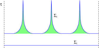
Figure 1: Evolution of the scale factor cutoff during structure formation. The constant scale factor time surface $\Sigma_{1}$ lies in the early, approximately homogeneous universe and coincides with a surface of constant FRW time $\tau$. As density perturbations grow, some geodesics decouple from the Hubble flow, stop expanding, and become trapped in collapsed regions such as galaxies. If the scale factor cutoff exceeds the largest scale factor ever reached along such geodesics, then the rule of De Simone et al. requires that their entire future evolution be included. (A similar result obtains if the local formulation of the scale factor measure is used as a general definition; see Sec. 5.4.) Therefore, the later cutoff surface $\Sigma_{2}$ no longer agrees everywhere with a constant FRW time surface; it includes the entire future of collapsed regions (green/gray), which show up as spikes since the figure is drawn in comoving coordinates.

The prescription for collapsed regions chosen by De Simone et al. is not the only possible one. Indeed, we will find that it has phenomenological disadvantages (Sec. V), and we will suggest other possible definitions. In particular, the local formulation of the scale factor measure (Sec. IV.2) applies without modification both in collapsing and expanding regions. However, we will not explore these alternatives in detail; we focus on the definition of Ref. DGSV08 in this paper.

There is another ambiguity, however, which has yet to be resolved. When a new vacuum with lower cosmological constant is formed by the Coleman-DeLuccia process, there is a quantum region, where the geometry (in the instanton approximation) jumps sharply and the continuation of geodesics is not well-defined. For downward tunnelings, one can reasonably ignore this problem, since the initial radius of the bubble wall can be much smaller than the de Sitter radius, so only a negligible fraction of geodesics entering the new bubble pass through the bubble interior at the time of nucleation. Moreover, geodesics quickly become comoving in regions with slow-roll inflation, which are of the greatest interest.

De Sitter vacua may also tunnel upward, to vacua with larger cosmological constant. Even though upward tunnelings are very suppressed, the scale factor measure implies that majority of observers live on world lines which have been through upward tunnelings Sch06 ; Sch08 . But there is no approximate classical geometry describing an upward tunneling. There is no natural way, therefore, of determining the tangent vectors of the portion of the geodesic congruence entering the new bubble.

For the purpose of deriving the rate equations, in Sec. II.2, we will follow Ref. GarSch05 and sidestep this issue by making mathematically convenient assumptions. Once we count observers in Sec. IV, the ambiguity will not re-enter: we are only interested in the most recent tunneling, which is necessarily downward for producing ordinary observers.

II.2 Rate equations and solutions

Before we can count observers in vacuum $i$, we will need to know the number $n_{i}(\eta)$ of such bubbles below the cutoff $\eta$. This, in turn, requires knowing the physical volume $V_{i}(\eta)$ occupied by every vacuum. The evolution and distribution of these volumes is determined by the rate matrix $\Gamma_{ij}$ describing the number of bubbles of vacuum $i$ forming per unit four volume of vacuum $j$.

For nonterminal vacua (i.e., those with positive cosmological constant $\Lambda_{i}$), the following definitions will be convenient: the expansion at late times,

$$H_{i}\equiv\left(\frac{\Lambda_{i}}{3}\right)^{1/2}~{};$$ (6)

the total decay rate of vacuum $i$ per unit four-volume,

$$\Gamma_{j}\equiv\sum_{i}\Gamma_{ij}~{};$$ (7)

the dimensionless decay rate from vacuum $j$ to $i$,

$$\kappa_{ij}\equiv\frac{4\pi}{3}\frac{\Gamma_{ij}}{H_{j}^{4}}~{};$$ (8)

the total dimensionless decay rate of vacuum $j$,

$$\kappa_{j}\equiv\sum_{i}\kappa_{ij}~{},$$ (9)

and the branching ratio matrix

$$\beta_{ij}\equiv\kappa_{ij}/\kappa_{j}~{}.$$ (10)

During a time interval $d\eta$, the volume $V_{i}$ in vacuum $i$ will increase due to intrinsic expansion, due to the production of new bubbles of type $i$, and due to the expansion of the bubble walls into the parent vacua. It will decrease due to decay into other vacua, and due to the growth of such bubble walls after they are produced.

Treating the motion of domain walls in detail is cumbersome, and it is unnecessary if all metastable vacua are long-lived ($\kappa_{i}\ll 1$). This is a reasonable assumption, since $\kappa_{i}\gg 1$ conflicts with the notion of a vacuum, and $\kappa_{i}\sim 1$ requires fine tuning. Such vacua will be too rare in the landscape to play an important dynamical role.

Thus, most of the four-volume of each bubble type is empty de Sitter space, and we can neglect transient effects right after bubble nucleation. One transient is the period between bubble creation and vacuum domination. Therefore, the expansion $\theta$ of geodesics in vacuum $j$ can be approximated by the Hubble constant at late times, $\theta\approx H_{j}\equiv(\Lambda_{i}/3)^{1/2}$. The four-volume in vacuum $j$ added during the scale factor time $d\eta$ is thus $V_{j}H_{j}^{-1}d\eta$.

Another transient is the bubble wall expansion. A bubble nucleated at the time $\eta^{\rm nuc}$ will eventually occupy a comoving volume in the geodesic congruence that would (in the absence of the decay) have originated from a ball of physical radius $H_{j}^{-1}$ in the parent vacuum $j$ at the time $\eta^{\rm nuc}$. This asymptotic comoving size is reached, to accuracy of order $\exp(\eta-\eta^{\rm nuc})$, after only a few units of scale factor time. Thus we make a small error by anticipating this growth: We ascribe a physical volume $4\pi/3H_{j}^{3}$ to the new vacuum $i$ already at the nucleation time $\eta^{\rm nuc}$, and in exchange neglect the bubble wall growth GarSch05 .

With these approximations, vacuum $i$ gains

$$d^{+}V_{i}=3V_{i}\,d\eta+\sum_{j}\left(V_{j}\frac{d\eta}{H_{j}}\right)\Gamma_{ij}\left(\frac{4\pi}{3H_{j}^{3}}\right)~{}.$$ (11)

and loses

$$d^{-}V_{i}=\sum_{j}\left(V_{i}\frac{d\eta}{H_{i}}\right)\Gamma_{ji}\left(\frac{4\pi}{3H_{i}^{3}}\right)~{}.$$ (12)

in physical volume per scale factor time. Combining inflow and outflow yields the Fokker-Planck equation

$$\frac{dV_{i}}{d\eta}=3V_{i}-\kappa_{i}V_{i}+\sum_{j}\kappa_{ij}V_{j}~{}.$$ (13)

Ref. GarSch05 rigorously derives the solution to this equation. Only the behavior of de Sitter vacua will be relevant here. For generic initial conditions with some support in de Sitter vacua, the solution approaches attractor behavior at late times. The volume in de Sitter vacuum $i$ is

$$V_{i}(\eta)=C\,s_{i}\,e^{\gamma\eta}~{}.$$ (14)

Here, $C$ is a constant with the dimension of volume that depends on the initial conditions but drops out in all normalized probabilities;

$$\gamma\equiv 3-q~{};$$ (15)

$q$ is the smallest-magnitude negative eigenvalue of the dimensionless flow matrix $\kappa_{ij}-\delta_{ij}\kappa_{i}$; and $s_{j}$ is the associated eigenvector:

$$\kappa_{ij}s_{j}=(\kappa_{i}-q)s_{i}\equiv p_{i}~{},$$ (16)

where we have defined the vector $p_{i}$ for later convenience.

To exponentially good approximation SchVil06 , the eigenvector is dominated by the longest-lived de Sitter vacuum, $*$:

$$s_{j}\approx\delta_{j*}~{};$$ (17)

and its eigenvalue is equal to the dimensionless decay rate of this vacuum,

$$q\approx\kappa_{*}\ll 1$$ (18)

Thus, $q$ is exponentially small in a realistic landscape.—By Eq. (2), this attractor solution is all we need to compute probabilities.

A number of other results will be useful below, and we collect them here. The expected number of times a worldline starting in vacuum $o$ vacuum will pass through vacuum $i$ can be obtained by summing over the whole branching tree Bou06 :

$$e_{io}=\delta_{io}+\sum_{{\rm paths~{}from}~{}o~{}{\rm to}~{}i}\beta_{ii_{n}}~{}\beta_{i_{n}i_{n-1}}~{}...~{}\beta_{i_{1}o}~{},$$ (19)

where $i_{1}...i_{n}$ are intermediate vacua connecting $o$ and $i$, and the branching ratios $\beta_{ij}$ were defined in Eq. (10). This can be written in matrix form as

$$e_{io}=\bigg{(}\sum_{n=0}^{\infty}\bm{\beta}^{n}\bigg{)}_{io}~{},$$ (20)

In the scale factor measure, the initial vacuum is the $*$ vacuum, and we will denote

$$e_{i}\equiv e_{i*}$$ (21)

If the initial vacuum has relatively small cosmological constant, as one might expect for the longest-lived vacuum, then it is unlikely to be re-entered later in the decay chain. Then the sum in Eq. (20) converges rapidly; in particular,

$$e_{*}\approx 1~{}.$$ (22)

In Ref. BouYan07 , the vectors $p_{i}$ and $e_{i}$ were shown to be closely related:

$$p_{i} = q\bigg{(}\sum_{n=1}^{\infty}\beta^{n}\bigg{)}_{ij}s_{j}$$ (23)

$$\approx q\bigg{(}\sum_{n=1}^{\infty}\beta^{n}\bigg{)}_{i*}~{}.$$

$$\approx qe_{i}~{}~{}~{}~{}~{}(i\neq*)$$

Note, however, that $p_{*}\neq qe_{*}$.

III The cutoff hypersurface in a homogeneous bubble

In this subsection, we investigate the evolution of the cutoff hypersurface in a single bubble of an arbitrary vacuum, nucleated inside a parent vacuum with positive cosmological constant $3H^{2}$. We will drop the index $i$ while discussing a single vacuum. For now, we will ignore inhomogeneities, such as density perturbations and local gravitational collapse.

Assuming that the tunneling process is very rare, the parent vacuum will have existed for a long time before the nucleation event. This implies GarGut06 that we can take the geodesic congruence to be comoving in the flat slicing of de Sitter space,

$$ds^{2}=-dt^{2}+e^{2Ht}(dr^{2}+r^{2}d\Omega^{2})~{}.$$ (24)

We can think of $r$ as labelling a particular shell in the congruence. The geodesics between $r$ and $r+\delta r$ span a volume element

$$\delta V(t,r)=\left.\frac{dV}{dr}\right|_{t=\rm{const}}\delta r=4\pi e^{2Ht}r^{2}\delta r$$ (25)

in the parent vacuum.

In the homogeneous approximation, the metric inside the bubble is described by an open FRW geometry

$$ds^{2}=-d\tau^{2}+a^{2}(\tau)(d\xi^{2}+\sinh^{2}\xi\,d\Omega_{2}^{2})~{}.$$ (26)

The comoving geodesics from the host vacuum continue into the bubble along nontrivial trajectories, defining a second coordinate system $(t,r)$ inside the bubble, where $t$ is the proper time along the geodesic passing through an event, and $r$ is the radial position the geodesic had before entering the bubble. We will now review the coordinate transformation between $(\tau,\xi)$ and $(t,r)$, derived in Ref. BouFre07 .

Without loss of generality, one can choose coordinates so that the bubble is nucleated at $t=0,r=0$. Consider a comoving geodesic which passes through the event $t=0,r$. If after a proper time $t$ (as measured along the geodesic) it has passed into the bubble, its coordinates $(\tau,\xi)$ will be

$$\xi(t,r) = -\log(1-Hr)+{\cal O}(\frac{1}{H\tau})$$

$$\tau(t,r) = t-\frac{\xi+e^{-\xi}-1}{H}+{\cal O}(\frac{1}{H\tau})~{}.$$ (27)

Note that $H$ in these formulas refers to the constant expansion rate of the parent de Sitter space. The above equations are valid for geodesics that have spent more than a proper time $H^{-1}$ inside the bubble. Physically, this result shows that the geodesics become comoving in the open coordinates after one outside Hubble time, and thereafter the proper time along the geodesics increases at the same rate as the open FRW time.

To construct the cutoff hypersurface, one must determine the scale factor time $\eta$ as a function of the bubble coordinates $\tau$ and $\xi$. By Eq. (14),

$$\eta(\eta^{\rm nuc},\tau,\xi)=\eta^{\rm nuc}+\frac{1}{3}\log\left(\frac{\delta V[r(\tau,\xi),t(\tau,\xi)]}{\delta V(r,0)}\right)~{},$$ (28)

where $\eta^{\rm nuc}$ is the scale factor time at $t=0$, when the bubble is nucleated. The volume element $\delta V$ orthogonal to the geodesics lies on a hypersurface of constant proper time $t$ Wald . By Eq. (26),

$$\delta V=$$

$$4\pi a^{2}(\tau)\sinh^{2}\xi\left[a^{2}(\tau)\left(\frac{d\xi}{dr}\right)_{t={\rm const}}^{2}-\left(\frac{d\tau}{dr}\right)_{t={\rm const}}^{2}\right]^{1/2}\delta r$$

$$=4\pi a(\tau)^{2}\sinh^{2}\xi\,\left[a(\tau)^{2}-\left(\frac{1-e^{-\xi}}{H}\right)^{2}\right]^{1/2}He^{\xi}\,\delta r~{},$$ (29)

where we have used Eq. (27). We are interested in events much later than the outside Hubble time, so $a^{2}\gg H^{-2}$, and we can drop the second term in the square root:

$$\delta V=4\pi Ha^{3}(\tau)e^{\xi}\sinh^{2}\xi\,\delta r$$ (30)

After using Eq. (27) to eliminate $r$ from Eq. (25), Eq. (28) yields the scale factor time inside the bubble:

$$\eta(\eta^{\rm nuc},\tau,\xi)=\eta^{\rm nuc}+\log\left[Ha(\tau)\right]+\frac{2}{3}\left[\xi+\log\left(\cosh\frac{\xi}{2}\right)\right]~{}.$$ (31)

IV Counting ordinary observers

In this section, we apply the scale factor cutoff to counting observations in an eternally inflating multiverse with multiple vacua. We exclude, for now, observations resulting from violations of the second law (Boltzmann brains, treated in Sec. VI). Initially, we will imagine that all observations (if any) in a bubble of type $i$ are made instantaneously at the FRW time $\tau^{\rm obs}_{i}$ after the vacuum is produced, with number density $\rho_{i}^{\rm obs}$ per unit physical volume:

$$dN_{i}=\rho_{i}^{\rm obs}dv_{\rm ph}~{}.$$ (32)

We will assume, moreover, that these parameters do not depend on the parent vacuum from which $i$ is entered. These assumptions will simplify our treatment, and it will be easy to drop them in the end and state a more general result, Eq. (43).

Our treatment will go beyond that of De Simone et al.  DGSV08 in that we do not approximate the bubble interior as flat and homogeneous. Our detailed treatment of collapsing regions, in Sec. IV.3, has significant implications, invalidating some of the conclusions of Ref. DGSV08 (see Sec. V).

IV.1 Counting observations in the no-collapse approximation

Now we will compute the total number of observations, $N_{i}(\eta)$, performed in vacua of type $i$ below the cutoff, $\eta$. By Eq. (32), this amounts to computing the total physical volume of the $\tau=\tau_{i}^{\rm obs}$ hypersurfaces below the cutoff. In any single bubble, a shell of comoving radius $\xi$ and width $d\xi$ contributes a physical volume

$$dv^{\rm ph}_{i}=4\pi(a_{i}^{\rm obs})^{3}\sinh^{2}\xi\,d\xi~{},$$ (33)

but only if the bubble was nucleated early enough for this volume to be included below the cutoff.

By Eq. (31), the latest nucleation time that allows observers at radius $\xi$ to contribute is

$$\eta_{ij}^{\rm nuc}(\eta,\xi)=\eta-\log\left[H_{j}a_{i}^{\rm obs}\right]-\frac{2}{3}\left[\xi+\log\left(\cosh\frac{\xi}{2}\right)\right]~{}.$$ (34)

Note that this time depends on the parent vacuum, $j$. Hence,

$$N_{i}(\eta)=\sum_{J}\int_{0}^{\infty}d\xi\,n_{ij}\!\left[\eta_{ij}^{\rm nuc}(\eta,\xi)\right]\,\frac{dv_{\rm ph}}{d\xi}(\xi)\,\rho_{i}^{\rm obs},$$ (35)

where $n_{ij}(\eta^{\prime})$ is the total number of bubbles of type $i$ nucleated inside vacuum $j$ by the time $\eta^{\prime}$.

Using

$$dn_{ij}=\Gamma_{ij}V_{j}d\eta/H_{j}$$ (36)

Eqs. (8) and (14) imply

$$n_{ij}(\eta_{ij}^{\rm nuc})=\frac{3C}{4\pi\gamma}H_{j}^{3}\kappa_{ij}s_{j}\exp(\gamma\eta_{ij}^{\rm nuc})~{}.$$ (37)

Combining the above equations, we find

$$N(\eta)=$$

$$\frac{3C}{4\pi\gamma}\left[\int_{0}^{\infty}d\xi\,4\pi\,\sinh^{2}\xi\,(\exp\xi)^{-2\gamma/3}\left(\cosh\frac{\xi}{2}\right)^{-2\gamma/3}\right]e^{\gamma\eta}$$

$$\times(a_{i}^{\rm obs})^{q}\left(\sum_{j}H_{j}^{q}\kappa_{ij}s_{j}\right)\rho_{i}^{\rm obs}~{}.$$ (38)

The $\xi$ integral is clearly convergent, with support concentrated near $\xi\sim O(1)$. (For small $q$, its value approaches $4\pi/3$.) Physically, this shows that mainly the central curvature volume of the infinite open bubble geometry contributes in the scale factor measure. Therefore, the interesting results of Garriga, Guth, and Vilenkin GarGut06 regarding worldlines at large $\xi$ are not relevant in this measure.

Since $q$ is exponentially small, $H_{j}^{q}$ and $(a_{i}^{\rm obs})^{q}$ can safely be neglected. By the discussion at the end of Sec. II, $\kappa_{ij}s_{j}=qe_{i}$. Thus we obtain the probability

$${\cal P}_{i}\propto e_{i}\,\rho_{i}^{\rm obs}~{}.$$ (39)

for observing vacuum $i$. The “$\propto$” notation indicates that the universal factor $\approx Cqe^{\gamma\eta}/\gamma$ has been dropped (since, by Eq. (2), it does not affect relative probabilities), though the probabilities have not been normalized.

Eq. (39) immediately implies several key properties of the scale factor measure:

• The probability for observing vacuum $i$ is simply the product of the number of times a typical worldline can be expected to enter $i$-bubbles, $e_{i}$, and the density, $\rho_{i}^{\rm obs}$, of observations per physical volume on the homogeneous timeslice $\tau_{i}^{\rm obs}$ at which they are performed.

• The probability of an observation depends on its FRW time, $\tau^{\rm obs}$, and on the FRW expansion factor at that time, $a^{\rm obs}$, only through $\rho^{\rm obs}$.

• As a special case, we recover an important result of De Simone et al. DGSV08 : Like in the causal diamond measure, the probability of a vacuum is insensitive to the volume expansion factor during slow-roll inflation. This is a desirable property, because it avoids the “Q-catastrophe” GarVil05 ; FelHal05 —the overwhelming pressure towards extreme (and counterfactual) inflationary parameter values that results when exponential volume factors are rewarded. Moreover, this property makes it conceivable that inflation was short enough to allow subtle signatures of the preceding era to survive, such as detectable curvature FreKle05 .

• Eq. (39) also captures another important result of Ref. DGSV08 , which we will examine in Sec. V: the probability of vacua where vacuum energy comes to dominate before $\tau_{i}^{\rm obs}$ is exponentially suppressed, because the matter density, $\rho_{{\rm matter},i}^{\rm obs}$, will have been diluted by the accelerated expansion. This, too, appears to replicate a success of the causal diamond measure: the suppression of moderately large values of the cosmological constant $\Lambda$, which are larger than the observed value but too small to affect the number of observers per matter mass. We will find, however, that this apparent success is an artifact of the no-collapse approximation.

Eq. (39) trivially generalizes to the case where observations are made at different different times $\tau_{\mu}$, $\mu=1,2,3\ldots$ The total probability to observe vacuum $i$ is

$${\cal P}_{i}\propto e_{i}\sum_{\mu}\rho^{\rm obs}_{i}(\tau_{\mu})~{},$$ (40)

where $\rho^{\rm obs}_{i}(\tau_{\mu})$ is the density of observations taking place at $\tau_{\mu}$. In the continuous case,

$${\cal P}_{i}\propto e_{i}\int_{0}^{\infty}d\tau\,\frac{d\rho^{\rm obs}_{i}}{d\tau}~{},$$ (41)

where the integrand is the number of observations made in the FRW time interval $(\tau,\tau+d\tau)$, per unit physical volume of the hypersurface $\tau$. If more differentiated observations are performed (for example, local conditions like temperature, rather than just a determination of the vacuum), $\rho_{i}$ can be given additional indices or arguments.

IV.2 The no-collapse scale factor measure as a local measure

In the no-collapse approximation, the scale factor measure can be reformulated as a local measure. By this we mean that the measure can be defined by averaging over an ensemble of individual worldlines, instead of constructing a particular global spacetime. (The causal diamond measure is an example of a local measure.)

This can be seen by the following argument, illustrated in Fig. 2. The predictions of the scale factor measure are dominated by the late-time attractor behavior of the universe. (An infinite number of observations are produced during this era, while only a finite number are produced earlier.) Thus, we may as well pick a late-time surface, $\Sigma_{\eta}$ with $\eta$ very large, and choose it as our initial surface, $\Sigma_{0}$. In other words, we redefine $\eta\to\eta-\Delta\eta$, $\Delta\eta\approx\infty$, making sure we already start in the asymptotic regime. This cuts out irrelevant transients and leads to a very simple picture.

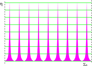
Figure 2: The green (light shaded) slices are surfaces of constant scale factor time, $\Sigma_{\eta}$; they have fixed comoving size but increasing physical volume. Fat geodesics (purple, dark shaded) have fixed physical width and thus decreasing comoving size. If the initial slice is chosen in the attractor regime, the fat-geodesics define a representative finite sample of the total four-volume. Thus, the results of the scale factor measure can be reproduced by following a single geodesic of fixed width, starting in the longest-lived metastable vacuum.

The volume occupied by long-lived metastable vacua on the late-time attractor hypersurface $\Sigma_{0}$ is dominated by empty de Sitter regions, with volume fraction $s_{i}$ allocated to vacuum $i$ GarSch05 . We can choose $\Sigma_{0}$ to be as large as we like, guaranteeing that it can be allocated the correct attractor volume fractions to arbitrary accuracy.

Now let us begin evolving forward along the congruence orthogonal to $\Sigma_{0}$. The scale factor measure instructs us to count observations in the four-volume thus generated, taking ratios as $\eta\to\infty$. Let us instead consider a reduced four-volume, $\tilde{V}_{4}$, which is finite, by dividing the initial surface $\Sigma_{0}$ into volume elements $dV$. As usual, we follow the geodesic orthogonal to each volume element. But we do not increase $dV$ as the universe expands. This creates a family of “fat geodesics”. At the time $\eta$, the fat geodesics occupy only a fraction $e^{-3\eta}$ of the total volume of $\Sigma_{\eta}$. But for every worldline, no matter in what type of region it started, the missing volume is exactly the same, $1-e^{-3\eta}$.

Because all fat geodesics expand by the same volume factor, the volume they do occupy on $\Sigma_{\eta}$ is a perfectly faithful sample of the hypersurface. (This is the crucial point—note, for example, that it would not hold in the attractor regime of the proper time measure.) Moreover, because this is true for every time interval $d\eta$, the four-volume swept out by the fat geodesics out is statistically equivalent to the four-volume between $\Sigma_{0}$ and $\Sigma_{\eta}$.

Therefore, reducing to $\tilde{V}_{4}$ will not affect probabilities:

$$\frac{{\cal P}(O_{i})}{{\cal P}(O_{j})}\equiv\lim_{\eta\to\infty}\frac{N_{i}}{N_{j}}=\frac{N_{i}(\tilde{V}_{4})}{N_{j}(\tilde{V}_{4})}~{},$$ (42)

where $V_{4}$ is obtained by following every geodesic to the asymptotic future. Instead of thinking about the actual collection of fat geodesics anchored on a large hypersurface, we may equivalently consider a statistical ensemble of single geodesics, with initial conditions weighted by the distribution of regions on a late-time attractor surface. Neglecting the rare regions occupied by recently nucleated bubbles, this means starting out with de Sitter vacuum $i$ with probability $s_{i}$. Because the vector $s_{i}$ is dominated by the $*$ vacuum, to a good approximation SchVil06 , this means starting the geodesic in the longest-lived metastable vacuum, $*$.

Thus, we reproduce the scale factor measure by following a single geodesic starting in $*$. The worldline evolves according to local dynamical laws, witnessing the decay of vacua and perhaps the production of observers, until it ends up in a terminal vacuum. We “fatten” the worldline, giving it a fixed physical cross-section, a volume element $dV$ orthogonal to the worldline. Finally, we compute the expectation value (ensemble average) of the differential number of observations of type $\mu$, $dN_{\mu}$, in the resulting four-volume:

$${\cal P}_{\mu}=\langle\rho_{\mu}\rangle~{},$$ (43)

where, for a given worldline in the ensemble,

$$\rho_{\mu}=\frac{dN_{\mu}}{dV}=\int dt\frac{dN_{\mu}}{dVdt}$$ (44)

We showed in Sec. III that geodesics quickly become comoving after entering a new bubble. Thus, the volume element $dV$ lies inside a constant-$\tau$ hypersurface of each FRW bubble universe. With the approximations used in Sec. IV.1, therefore, $\rho_{\mu}$ is identical to the physical density of observers, $\rho_{i}^{\rm obs}$, in vacuum $i$. The factor $e_{i}$ is captured by averaging over different worldlines in the ensemble BouYan07 , so Eq. (43) reduces to Eq. (39) as a special case. The more general Eqs. (40) and (41), too, are special cases of Eq. (43).

It would be interesting to use Eq. (43) as the defining equation of a measure. This would have a number of formal advantages. One geodesic carries much less geometric information than a whole congruence, so we face fewer ambiguities about the treatment of upward jumps. Moreover, Eq. (43) can be applied without modification in collapsing regions, whereas the formulation based on integrating the expansion along a geodesic congruence requires an additional, ad hoc, prescription to deal with such regions. Finally, the use of Eq. (43) to define a measure liberates us from the initial conditions $s_{i}$ picked out by the attractor regime of the geodesic congruence. Starting the fat geodesic with initial conditions that favor Planck-scale vacua, for example, would avoid the potential “staggering problem” associated with the enormous suppression of the upward jumps from the dominant vacuum $*$.

IV.3 Proper treatment of collapsed regions

At least in our own bubble, some observations are made in collapsed regions. The FRW metric, Eq. (26), does not capture the local geometry of such regions, but provides only an average over scales on which the universe can be considered homogeneous. Hence, this metric cannot be used to compute the local scale factor, $A$, and the scale factor time, $\eta$, along geodesics entering collapsed regions such as galaxies. Despite the similar names, the FRW scale factor $a$ and the local scale factor $A$ are two completely different objects.

Geodesics that end up in dark matter haloes will, by definition, have ceased to expand, and decoupled from the Hubble flow, before the halo formed. After reaching a maximum expansion, they will have turned around and collapsed, with $A$ and $\eta$ decreasing during the collapse. These geodesics will reach observers, but their maximum scale factor $A_{\rm max}$ will be unrelated to the FRW scale factor at the time $t_{\rm obs}$, $a_{\rm obs}$. Rather, it will be related to the FRW scale factor at the time of structure formation, $a_{\rm NL}$.

Consider a simple, spherically symmetric model. A dark matter halo forms by the collapse of a spherical overdensity. Then baryons fall into its gravitational well, cool, and condense in the center. Eventually the gas fragments into stars.

Let us focus on the dark matter particles that end up in the halo. Initially, each particle follows one of the geodesics in the congruence that defines the scale factor cutoff. The maximum scale factor is achieved at the time of turnaround, when all the dark matter particles are momentarily stationary. Note that it is smaller than, but on the order of, the FRW scale factor $a$ at the time of turnaround.

After the turnaround, the particles fall towards the center of the halo. Depending on interactions, the particles will eventually stop following the geodesics, but in the spherical model, the geodesics remain very simple. They will focus in the center of the halo, and begin expanding again, back out to the turnaround radius; this pattern will be repeated indefinitely. The entire congruence of geodesics will keep oscillating about the center of the halo, with an amplitude given by the turnaround radius. This radius is twice the virial radius, and perhaps ten times the eventual galaxy radius. Therefore, the congruence continues to thread the galaxy at all times. Crucially, it will capture observers independently of how long it takes to form them.

With a more realistic structure formation model, the situation would appear to be even more clear cut. Generic geodesics will remain gravitationally bound to the halo, but will be spread chaotically through micro-lensing. (This means that the same event will lie on multiple geodesics, but as discussed above, we will count each event only once.) Moreover, most large halos do not form directly from from a single overdensity, but by mergers and accretion of smaller halos that virialized much earlier. One expects that most geodesics threading merging halos will remain gravitationally bound during the merger, and end up covering the resulting larger galaxy. But then observers will have a local scale factor which is less than the averaged scale factor at the time of the formation of the smallest structures that eventually merge to form our galaxies. Note that these structures need not even be galaxies, i.e., their mass could be below $10^{7}$ solar masses.

The measure defined by De Simone et al. instructs us to include all observations reached by geodesics whose maximum scale factor time is below the cutoff. Therefore, all observations in collapsed regions will contribute as soon as the cutoff exceeds the maximum local scale factor of the first collapsing objects that end up constituting the host objects of observations.

To include this effect, one could generalize to a more detailed metric. But it is much simpler to continue working with the homogeneous FRW metric, Eq. (26), and to include collapse effects by pretending that all observations in collapsed regions happen at the time $\tau^{\rm NL}$ when those regions decoupled from the Hubble flow. This amounts to projecting observations from the time $\tau^{\rm obs}$ back to the earlier time $\tau^{\rm NL}$, and thus, to increasing their number density per physical volume to

$$\hat{\rho}_{i}^{\rm obs}\equiv\rho_{i}^{\rm obs}\left(\frac{a_{i}^{\rm obs}}{a_{i}^{\rm NL}}\right)^{3}~{},$$ (45)

where $a_{i}^{\rm NL}\equiv a(\tau_{i}^{\rm NL})$.

Thus, we can include the effects of local collapse by replacing Eq. (39) by

$${\cal P}_{i}\propto e_{i}\,\hat{\rho}_{i}^{\rm obs}~{}.$$ (46)

V The cosmological constant

In this section, we estimate the probability distribution for the cosmological constant in the scale factor measure. We will find that it agrees roughly with the observed value in the no-collapse approximation. Treating collapsed regions according to the prescription of De Simone et al., however, yields a much larger value. We will then consider variations of the scale factor measure and discuss how they might solve this problem. Let us begin by reviewing the history of anthropic predictions for the cosmological constant and how they depend on the measure.

Throughout this paper, we will focus on positive values of $\Lambda$, which have a greater potential for discrepancy with observation. Negative values of $\Lambda$ are bounded (in any non-pathological measure; for example, if there is no youngness paradox) by the order of magnitude of the observed value, but positive values could be much larger Wei87 . Both the causal diamond measure BouHar07 and the no-collapse scale factor measure DGSV08 assign somewhat higher integrated probability to negative values than to positive values of $\Lambda$, but the imbalance is not large enough to render the observed value unlikely.

V.1 $\Lambda$ and observers per baryon

In anthropic approaches to the cosmological constant problem, one computes a probability distribution for observed values of the cosmological constant. Originally Efs95 ; Vil95 ; Wei96 ; MarSha97 ; Vil04 ; GarSch05 ; Wei05 this was implemented by multiplying the underlying distribution (arguably, $dp/d\Lambda=$ const in the regime of interest) by the “number of observers per baryon”, or per some other reference object. Implicitly, this defines an (incomplete) measure. If one tries to take “observers per baryon” seriously as a measure, one finds that any eternally inflating de Sitter vacuum has an infinite number of observers per baryon (if it has any observers at all), and 100% of the observers are Boltzmann brains Pag06 ; BouFre06b .

Even aside from this problem, however, the observer-per-baryon measure was already plagued by some annoying problems. The simplest test of the landscape solution to the cosmological constant problem is to restrict attention to vacua that differ from ours only through their value of $\Lambda$. In this setting, the observer-per-baryon measure prefers values of $\Lambda$ about 5000 times larger than the observed value; the observed value is excluded at the $3.5\sigma$ level BouHar07 . We find it useful to explain this in terms of the timescale

$$\tau_{\Lambda}=\sqrt{\frac{3}{\Lambda}}$$ (47)

at which the cosmological constant comes to dominate the evolution of the universe. In the observer-per-baryon measure, the number of observers will be proportional to the number of baryons that are captured by galaxies. The underlying distribution prefers larger values of $\Lambda$. There is no penalty until $\Lambda$ becomes large enough to disrupt galaxy formation ($\tau_{\Lambda}\ll\tau_{\rm gal}$); such values will be strongly suppressed. Thus one would expect $\Lambda$ to be correlated with the time of the formation of the first galaxies, $\tau_{\rm gal}$:

$$\Lambda\sim\tau_{\rm gal}^{-2}~{}.$$ (48)

In fact, however, the observed value of $\Lambda$ appears to be correlated with the (considerably later) time when observations are made, $\tau_{\rm obs}$:

$$\Lambda\sim\tau_{\rm obs}^{-2}\sim 10^{-4}\tau_{\rm gal}^{-2}~{}.$$ (49)

This is the coincidence problem. The observers-per-baryon measure (ignoring Boltzmann brains) would have naturally explained a hypothetical coincidence between $\tau_{\rm gal}$ and $\tau_{\Lambda}$, but it is only barely consistent with the actual coincidence between $\tau_{\rm obs}$ and $\tau_{\Lambda}$.

Further tests can be made by allowing other parameters (such as the density contrast, curvature, etc.) to vary in addition to $\Lambda$, or by integrating out such parameters altogether. This exacerbates the troubles of the observer-per-baryon measure. For example, it strongly prefers larger values of the density contrast, $Q$, than the observed value $Q\sim 2\times 10^{-5}$. Since $\tau_{\rm gal}\propto Q^{-3/2}$, vacua with larger $Q$ can tolerate larger $\Lambda$ (like $Q^{3}$) while still forming structure. Thus, a greater fraction of such vacua contains observers, and they are strongly preferred.

V.2 $\Lambda$ and the causal diamond measure

The causal diamond measure Bou06 ; BouFre06a was the first to solve these problems. Most directly, it solves the coincidence problem, predicting a value of $\Lambda$ such that $\tau_{\Lambda}\sim\tau_{\rm obs}$, or $\Lambda\sim\tau_{\rm obs}^{-2}$. Greater values of $\Lambda$ are suppressed mainly because observers become exponentially dilute within the cutoff BouHar07 :

$$\frac{d{\cal P}}{d\log\Lambda}\propto\Lambda^{1/2}\exp\left(-\frac{3\tau_{\rm obs}}{\tau_{\Lambda}}\right)~{}.$$ (50)

Using $\tau_{\rm obs}\sim O(10$ Gyr$)$ (or alternatively, and less anthropocentrically, equating the peak observation time with the time of peak entropy production), this relation leads to a prediction of $\Lambda$ in excellent agreement with the observed value. Because the causal diamond measure correlates $\Lambda$ directly with the era when observations are made, and not with the time when structure forms, the $Q$ runaway problem is absent BouHar07 ; CliFre07 .

V.3 $\Lambda$ and the scale factor measure

De Simone et al. DGSV08 have argued that the scale factor measure shares some of these desirable properties. We will now examine this claim, focusing, once more, on the case where only $\Lambda$ varies, while keeping $\tau_{\rm obs}$ fixed. We will find that the conclusions of De Simone et al. apply in the no-collapse approximation, but are invalidated by collapse effects.

V.3.1 No-collapse approximation

In the no-collapse approximation adopted in Ref. DGSV08 , Eq. (39) tells us that

$$\frac{d{\cal P}}{d\Lambda}\propto\frac{dp}{d\Lambda}\rho^{\rm obs}(\Lambda)$$ (51)

We assume that $dp/d\Lambda$ is constant in a small interval (say, $10^{-20}$) around $\Lambda=0$, after coarse graining over an even smaller interval (say, $10^{-130}$). If this is not the case, then the landscape cannot solve the cosmological constant problem, and the scale factor measure would be ruled out. Hence we may drop this factor and write

$$\frac{d{\cal P}}{d\log\Lambda}\propto\Lambda\,\rho^{\rm obs}(\Lambda)~{}.$$ (52)

To understand how the observer density depends on $\Lambda$, let us rewrite $\rho^{\rm obs}$ as a fraction of the physical matter density at the time of observations,

$$\rho^{\rm obs}(\Lambda)=\alpha(\Lambda)\,\rho_{\rm matter}^{\rm obs}(\Lambda)~{},$$ (53)

so that

$$\frac{d{\cal P}}{d\log\Lambda}\propto\Lambda\,\alpha(\Lambda)\,\rho_{\rm matter}^{\rm obs}(\Lambda)~{},$$ (54)

It is reasonable to assume that $\alpha$, the number of observers per unit matter mass, is proportional to the Press-Schechter mass function MarSha97 , the fraction of matter mass in collapsed objects above a certain critical mass ($10^{7}$ solar masses for the smallest galaxies; more if one makes the additional anthropic assumption that observers require particularly large galaxies). To first approximation, $\alpha$ is unaffected by $\Lambda$ as long as $\tau_{\Lambda}\gg\tau_{\rm gal}$. Larger values of $\Lambda$ will noticaby affect galaxy formation, and for $\tau_{\Lambda}\ll\tau_{\rm gal}$, $\alpha$ rapidly vanishes.

The matter density at the time of observations is independent of $\Lambda$ as long as $\tau_{\Lambda}\gg\tau_{\rm obs}$. But if $\Lambda$ comes to dominate earlier, then it will drive a period of exponential expansion before observations are made, and the matter density will be far lower. Roughly, we can write

$$\rho_{\rm matter}^{\rm obs}(\Lambda)\approx\rho_{\rm matter}^{\rm obs}(\Lambda=0)~{}\exp\left(-3\,\frac{\tau_{\rm obs}}{\tau_{\Lambda}}\right)~{}.$$ (55)

For example, in vacua with $\tau_{\Lambda}\approx 2$ Gyr, the density of galaxies at $\tau_{\rm obs}\approx 13.7$ Gyr will a factor of order $10^{-9}$ times smaller than in vacua with $\tau_{\Lambda}\gg 13.7$ Gyr. Thus, moderately large values of $\Lambda$ are totally suppressed, even though they do not disrupt galaxy formation. We conclude that in the no-collapse approximation, the suppression of large $\Lambda$ is dominated by the dilution of matter, and one obtains

$$\frac{d{\cal P}}{d\log\Lambda}\propto\Lambda\exp\left(-3\,\frac{\tau_{\rm obs}}{\tau_{\Lambda}}\right)~{}.$$ (56)

Comparison with Eq. (50) reveals that the exponential factor is the same as that arising in the causal diamond measure. In both measures, this factor arises primarily from the effect of $\Lambda$ on the matter density, rather than its effect on galaxy formation. The prefactors differ because the physical volume of the causal diamond also depends on $\Lambda$, like $\Lambda^{-1/2}$ for large $\Lambda$. (In both cases the prefactor contains a factor $\Lambda$ from the Jacobian $d\log\Lambda/d\Lambda$.) Both distributions peak near $\Lambda\sim\tau_{\rm obs}^{-2}$, in excellent agreement with observation, Eq. (49).

V.3.2 Proper treatment of collapsed regions

With the proper treatment of collapsed regions, however, the result changes drastically. Eq. (39) is replaced by Eq. (46), and correspondingly, we must replace Eq. (52) by

$$\frac{d{\cal P}}{d\log\Lambda}\propto\Lambda\hat{\rho}^{\rm obs}(\Lambda)~{},$$ (57)

where $\hat{\rho}^{\rm obs}$ is the density, per physical volume, that observations would have had if they had occurred at the time $\tau_{\rm NL}$ when the first dark matter halos decoupled from the Hubble flow. By Eqs. (45) and (53), it follows that

$$\frac{d{\cal P}}{d\log\Lambda}\propto\Lambda\,\alpha(\Lambda)\,\rho_{\rm matter}^{\rm NL}(\Lambda)~{},$$ (58)

where $\rho_{\rm matter}^{\rm NL}$ is the physical matter density at the time $\tau_{\rm NL}$.

This matter density is insensitive to $\Lambda$ unless $\Lambda$ is large enough to affect the formation of the earliest dark matter haloes, at the time $\tau_{\rm NL}$. Since $\tau_{\rm NL}<\tau_{\rm gal}$, the dilution of matter density is now no longer the effect suppressing large $\Lambda$. Rather, it is disruption of galaxy formation: the Press-Schechter factor, which enters through $\alpha$. It becomes suppressed if $\Lambda$ exceeds $\tau_{\rm gal}^{-2}$, so the distribution will peak near this value.

Thus, the scale factor measure reproduces the result obtained from the observers-per-baryon measure, Eq. (48), except for the latter measure’s manifest Boltzmann brain problem. It prefers a value of $\Lambda$ that is, depending on the strength of anthropic assumptions, one to four orders of magnitude larger than the observed value.

Moreover, the scale factor measure suffers from a runaway problem if the strength of initial density perturbations, $Q$, is allowed to vary. The pressure towards large $Q$ is actually greater than in the observers-per-baryon measure. In both measures, larger $Q$ allows for larger values of $\Lambda$, since the maximum vacuum energy is of order the density at the time of galaxy formation, which is proportional to $Q^{3}$. This enters through the first factor in Eq. (58), suppressing the probability of the observed value of $\Lambda$ by an additional factor $(Q_{0}/Q)^{3}$. But in the scale factor measure, the last factor in Eq. (58) offers an additional reward for large $Q$: the density at the time of the earliest halo formation also scales like the third power of $Q$. This makes it more difficult to compensate for the runaway problem by prior distributions or anthropic cutoffs.

V.4 Can the scale factor measure be improved?

We have found that the scale factor measure predicts $\Lambda\sim\tau_{\rm gal}^{-2}$, while the causal diamond measure predicts $\Lambda\sim\tau_{\rm obs}^{-2}$. Can we pinpoint the key difference between the measures leading to these different results? And can the definition of the scale factor measure be modified to yield a more desirable answer?

The causal diamond measure is defined nonlocally, in terms of the event horizon of a single worldline. Observations inside this horizon will be included, those outside will not. The horizon size is not affected by local phenomena such as gravitational collapse. If $\tau_{\Lambda}\ll\tau_{\rm obs}$, then observations will be dilute, and few if any will be captured by the diamond.

The scale factor measure is defined in terms of a local quantity, the expansion and local scale factor of a congruence of geodesics. The local scale factor runs backwards once structure formation begins, and a special rule is needed to decide how the cutoff should be specified in this case. By the rule of De Simone et al., future observations occurring on such geodesics are immediately counted at structure formation, so the dilution of galaxies by the cosmological constant cannot affect the probability distribution.

One might attempt to improve the scale factor measure by replacing the local scale factor, $A$, with the averaged scale factor, $a$, describing the spatial curvature radius in expanding open FRW bubbles, while a geodesic is passing through matter dominated regions (up to an obvious constant factor that depends on the scale factor time at which the geodesic enters the matter dominated region). The idea would be to avoid the effects of collapse by averaging over collapsed regions and defining the scale factor time in terms of the averaged Hubble flow.

A problem with this approach is that the FRW scale factor $a$ is only approximately defined. On the scales currently within the horizon, there exists a preferred slicing of constant average density, which defines hypersurfaces of constant $a$. However, because the universe is not exactly homogeneous and isotropic, the averaging procedure is necessarily somewhat ambiguous—in the observable universe, at least at the level of $10^{-5}$. At larger scales, or in different bubbles, density fluctuations can be much larger. Bubbles with eternal slow-roll inflation cannot be assigned a preferred FRW slicing at all; neither can the asymptotic regions containing Boltzmann brains. Thus, it is unclear how this idea would lead to a sufficiently general prescription for computing probabilities.

A more promising approach to improving the scale factor measure is to change the rule that deals with collapsing geodesics, so that observers are not counted by geodesics that turn around too early. For example, whenever an event is passed through by multiple geodesics, we might assign its scale factor time to be the maximum scale factor time among those geodesics. This is in principle as well-defined as the proposal in DGSV08 , which corresponds to using the minimum. A closely related idea is to extend each geodesic only until its first caustic, when neighboring geodesics intersect and $\theta\to-\infty$. Whether such prescriptions lead to a better prediction for $\Lambda$ is an interesting question, but one beyond the scope of the present paper.

Finally, we may turn to the local formulation of the scale factor measure, Eq. (43), for help. In expanding regions, it is equivalent to the formulation using a geodesic congruence, but as noted at the end of Sec. IV.2, the local formulation can be applied without modification in collapsed regions. It would, however, suffer from a similar problem with predicting $\Lambda$. Most “fat geodesics” are captured by dark matter halos around the time when those objects first form. Therefore, the expected density of observations is set by the matter density inside galaxies, and not by the large scale average of the matter density of the FRW solution at the time of observations, $\tau_{\rm obs}$. As a result, Eq. (43) is insensitive to the value of the cosmological constant unless it is large enough to disrupt galaxy formation. It would predict $\Lambda\sim\tau_{\rm gal}^{-2}$, in poor agreement with the observed value $\Lambda\sim\tau_{\rm obs}^{-2}$.

Still, Eq. (43) may turn out a useful starting point for a more successful measure. Instead of fattening the geodesic infinitesimally, for example, we could consider constructing a larger transverse volume. We can then either attempt to take a large volume limit, in which the average density may become sensitive to the dilution caused by early vacuum domination. (Whether this can be done in a well-defined manner is, again, a question beyond the scope of our present work.) Or we could use a finite transverse volume. To avoid explicitly introducing an arbitrary length scale into the measure, this volume could be defined in terms of the cosmological event horizon surrounding the worldline. This fixes the $\Lambda$ problem, but it fails to produce a novel measure: With this prescription, we would simply recover the causal-diamond measure (with a particular choice of initial conditions).

VI Boltzmann brains

In this section, we compute the number of Boltzmann brains, and determine the conditions under which they dominate over ordinary observers. We define Boltzmann brains as observers that arise from local violations of the second law of thermodynamics. This occurs at late times in de Sitter vacua. States of energy $E\gg T$ are produced at the Boltzmann-suppressed rate

$$\Gamma_{i}(E)={4\pi\over 3}H_{i}^{4}\exp(-E/T_{i})$$ (59)

where $T_{i}=H_{i}/2\pi$ is the Gibbons-Hawking temperature of the de Sitter horizon. The minimum mass of a Boltzmann brain (if any) will depend on the vacuum. But on general grounds Bou00b ; BouFre06b , the exponential factor cannot be larger (though it can be much smaller) than $\exp(-S_{\rm BB})$, where $S_{\rm BB}$ is the course-grained entropy, or number of particles, in the most primitive Boltzmann brain,

$$\Gamma_{i}^{\rm BB}<\exp(-S_{\rm BB})~{}.$$ (60)

One can only speculate about the value of $S_{\rm BB}$, but it is certain to be exponentially large. Thus, Boltzmann brains are double-exponentially suppressed.

VI.1 The ratio of Boltzmann brains to ordinary observers

We can neglect crunching vacua, as well as the initial non-de Sitter regime of metastable vacua: because of the enormous suppression of Boltzmann brains, almost all of them will be produced in the asymptotic de Sitter regime. The number of Boltzmann brains produced in vacuum $i$ between the time $\eta$ and $\eta+d\eta$ is

$$dN_{i}^{\rm BB}=\Gamma^{\rm BB}_{i}V_{i}d\eta/H_{i}~{}.$$ (61)

By Eq. (14), the total number of Boltzmann brains produced prior to the cutoff $\eta$ in vacuum $i$ is therefore

$$N_{i}^{\rm BB}=\frac{Ce^{\gamma\eta}}{\gamma}\frac{s_{i}}{H_{i}}\Gamma^{\rm BB}_{i}~{}.$$ (62)

By Eqs. (17) and (16), $s_{*}\approx 1$ for the dominant vacuum and $s_{i}=p_{i}/(\kappa_{i}-q)\approx p_{i}/\kappa_{i}$ for all other vacua. Dropping the usual factor $Ce^{\gamma\eta}/\gamma$, the total probability for observations by Boltzmann brains is

$${\cal P}^{\rm BB}\propto H_{*}^{-1}\Gamma^{\rm BB}_{*}+\sum_{i\neq*}H_{i}^{-1}p_{i}\frac{\Gamma^{\rm BB}_{i}}{\kappa_{i}}~{}.$$ (63)

We are interested in comparing this to the total number of observations by ordinary observers,

$${\cal P}^{\rm OO}_{i}\propto\sum_{i}p_{i}\rho^{\rm OO}_{i}$$ (64)

The key simplification arising in this comparison is that $p_{i}$, $\Gamma^{\rm BB}_{i}$, and $\Gamma_{i}$, are generically double exponentials. That is, they are of the form $\exp(\pm\exp x)$ with $x\gg 1$. We will use a triple inequality sign for such numbers, for example

$$\Gamma^{\rm BB}\lll 1$$ (65)

Such numbers obey special laws of arithmetic. For example, for $y$ and $z$ double-exponentially large, $y/z\approx y$ if $y>z$. Moreover, if $y$ is a single exponential and $z$ a double exponential, then $zy\approx z/y\approx z$. A double exponential takes the same value in any conventional system of units, though it can be useful to think in terms of Planck units for definiteness.

The landscape contains an exponentially large number of vacua, but so far there are no indications that it might be doubly-exponentially large. Thus, $H_{i}$ is at most a single exponential, and we can write

$$\frac{{\cal P}^{\rm BB}}{{\cal P}^{\rm OO}}\approx\frac{\Gamma_{*}^{\rm BB}+\sum_{i\neq*}p_{i}~{}(\Gamma_{i}^{\rm BB}/\Gamma_{i})}{\sum_{i}p_{i}\,\rho^{\rm OO}_{i}}$$ (66)

Note that we have retained $\rho_{i}^{\rm OO}$, since it can be zero or doubly-exponentially small in some vacua. Because Eq. (66) involves a ratio of double exponentials, either the numerator or the denominator will completely dominate (depending on the measure, and on the landscape), and the relative probability will be zero or infinity to good approximation. Whoever wins, wins big.

We can restate this result in terms of the expected number $e_{i}$ of times a worldline starting in the $*$ vacuum will pass through vacuum $i$ (see the discussion at the end of Sec. II). Using $q\approx\kappa_{*}$, we can include the $*$ vacuum in the sum:

$$\frac{{\cal P}^{\rm BB}}{{\cal P}^{\rm OO}}\approx\frac{\sum_{i}e_{i}~{}(\Gamma_{i}^{\rm BB}/\Gamma_{i})}{\sum_{i}e_{i}\,\rho^{\rm OO}_{i}}~{}.$$ (67)

At this level of approximation, the causal diamond measure yields nearly the same result BouFre06b . In the causal diamond measure, the number of Boltzmann brains in vacuum $i$ is the expected number of times the generating worldline enters vacuum $i$, $e_{i}$, times $\Gamma^{\rm BB}_{i}$, times the expected four-volume the diamond will span in vacuum $i$ (given by the life-time of vacuum $i$, $H_{i}^{-1}\kappa_{i}^{-1}$, times the de Sitter horizon volume, $4\pi/3H_{i}^{3}$). The expected number of ordinary observers is $e_{i}$ times the number of ordinary observers inside the de Sitter horizon of vacuum $i$. Keeping only double-exponentials, the relative probability in the causal diamond measure is again given by Eq. (67).

Aside from negligible non-double-exponential factors, the only way the two measures differ, for the purposes of Boltzmann brains, is through $e_{i}$, which depend on initial conditions. A priori, the question of initial conditions has nothing to do with the measure problem, and in the causal diamond measure, they remain separate issues. One imagines that the universe started, perhaps, in a randomly chosen vacuum, or in an ensemble governed by the tunneling wavefunction, favoring Planck-scale vacua. Physical probabilities are not strongly affected by this uncertainty BouYan07 . In the scale factor measure, on the other hand, the eternally inflating universe exhibits attractor behavior, which can be mimicked by choosing the particular initial probability distribution $s_{i}$, defined in Sec. II. Roughly, this means starting the worldline in a very particular vacuum: the longest-lived metastable vacuum SchVil06 , $*$.

VI.2 Under what conditions do Boltzmann brains dominate?

In this subsection, we will show that with some reasonable assumptions about the landscape, the ratio of Boltzmann brains to ordinary observers takes an even simpler form. Except for the $*$ term, each term in the numerator of Eq. (66) contains the ratio $\Gamma_{i}^{\rm BB}/\Gamma_{i}$. By the laws of double exponential arithmetic, this ratio is dominated by the larger of the two exponents,

$${\Gamma_{i}^{\rm BB}\over\Gamma_{i}}\approx\left\{\begin{array}[]{rcl}\Gamma_{i}^{\rm BB}&<&\exp(-S_{\rm BB})\ \ {\rm if}\ \Gamma_{i}^{\rm BB}<\Gamma_{i}\\ \Gamma_{i}^{-1}&>&\exp(+S_{\rm BB})\ \ {\rm if}\ \Gamma_{i}^{\rm BB}>\Gamma_{i}\end{array}\right.~{},$$ (68)

where we have used Eq. (60) for the inequalities.

We will now constrain the factor $p_{i}$ multiplying this ratio. With no loss of generality, we may restrict the sum in Eq. (66) to the set of vacua containing observers or Boltzmann brains. Let us label the vacua in this set by the index $a$ instead of $i$. By Eqs. (19) and (23), $p_{a}$ can be obtained by a sum, over all decay paths, of products of branching ratios.

$$p_{a}=q\sum_{{\rm paths~{}from}~{}*~{}{\rm to}~{}a}\beta_{ai_{n}}~{}\beta_{i_{n}i_{n-1}}~{}...~{}\beta_{i_{1}*}~{}~{}~{}(a\neq*)~{},$$ (69)

This equation holds only for $a\neq*$, but those are precisely the $p_{a}$ appearing in Eq. (66).

We will make three assumptions:

• For every vacuum $a$, every decay path from $*$ to $a$ contains at least one intermediate de Sitter vacuum.—This assumption is very plausible in a multidimensional landscape such as that of string theory, where neighboring vacua have vastly different values of the cosmological constant (a crucial feature for solving the cosmological constant problem BP ; TASI07 ). Assuming that distant vacua cannot be accessed with appreciable probability, it follows that $\Delta\Lambda\gg 1/S_{\rm BB}$ in direct decays, so it is exponentially unlikely that the dominant vacuum can decay to any vacuum large enough to contain observers or Boltzmann brains.

• For every vacuum $a$, there exists at least one decay path from $*$ to $a$ which does not pass through any de Sitter vacua with horizon entropy bigger than $S_{\rm BB}$.—This assumption, too, is plausible given the scarcity of vacua with $\Lambda\ll 1$, and given our ability to choose any path we like.

• Of the decay paths posited in assumption (2), at least one “dominates” the sum in Eq. (69), in the following extremely weak sense: By dropping all other terms, we change the sum by less than a double exponential factor.—Like assumption (1), this is plausible in a multidimensional landscape with large step size, where decay chains in the semi-classical regime are short.

We remain agnostic about whether the $*$ vacuum has horizon entropy larger or smaller than $S_{\rm BB}$. The dominant vacuum is special. It is at least conceivable that its defining properties strongly select for a very small cosmological constant, and we do not wish to prejudice this issue here.

We will be interested in bounding $p_{a}$ only to within double-exponentially large factors. By assumption (3), we can drop the sum over paths and write

$$p_{a}\sim q~{}\beta_{ai_{n}}~{}\beta_{i_{n}i_{n-1}}~{}...~{}\beta_{i_{1}*}~{}~{}~{}(a\neq*)~{},$$ (70)

Assumption (1) guarantees that that $n\geq 1$, so $\beta_{i_{1}*}$ exists in the product and represents the branching ratio from one de Sitter vacuum to another. For two connected de Sitter vacua, detailed balance gives $\kappa_{i_{1}*}=\kappa_{*i_{1}}\exp(S_{i_{1}}-S_{*})$ where $S_{j}$ is the horizon entropy of vacuum $j$. Also, the decay rate must be faster than the recurrence time, $\kappa_{i_{1}*}>\exp(-S_{*})$. We are only considering vacua which eternally inflate, $\kappa_{*i_{1}}<1$, so

$$\exp(-S_{*})<\kappa_{i_{1}*}<\exp(S_{i_{1}}-S_{*})~{}.$$ (71)

We can divide by $\kappa_{*}$ to get a bound on the branching ratio,

$${1\over\kappa_{*}}\exp(-S_{*})<\beta_{i_{1}*}<{1\over\kappa_{*}}\exp(-S_{*}+S_{i_{1}})~{}.$$ (72)

For the other branching ratio(s) appearing in Eq. (70), we can use the cruder bound

$$\exp(-S_{j})<{1\over\kappa_{j}}\exp(-S_{j})<\beta_{ij}<1~{},$$ (73)

which holds also if the destination vacuum is terminal (as $a$ might be). Substituting these bounds into Eq. (19), we obtain

$$\exp(-S_{*})\exp(-S_{i_{1}}-S_{i_{2}}-...-S_{i_{n}})<p_{a}<\exp(-S_{*}+S_{i_{1}})~{},$$ (74)

where we have used $\kappa_{*}\approx q$. By assumption (2) (and assuming that the path is not exponentially long), we have $\sum_{k=1}^{n}S_{i_{k}}\ll S_{\rm BB}$, so

$$\exp(-S_{*})\exp(-S_{\rm BB})\lll p_{a}\lll\exp(-S_{*})\exp(+S_{\rm BB})~{}.$$ (75)

(We remind the reader that we use the triple inequality sign for the inequality of double exponentials.)

We have bounded $p_{a}$ to within a range small compared to $\exp(S_{\rm BB})$. Meanwhile, by Eq. (68), the ratio $\Gamma_{i}^{\rm BB}/\Gamma_{i}$ is either larger than $\exp(S_{\rm BB})$ or smaller than $\exp(-S_{\rm BB})$. By double exponential arithmetic, therefore, we can neglect the uncertainty in $p_{a}$ when we multiply these terms:

$$p_{a}{\Gamma_{a}^{\rm BB}\over\Gamma_{a}}\approx\exp(-S_{*}){\Gamma_{a}^{\rm BB}\over\Gamma_{a}}$$ (76)

By similar double exponential reasoning we can do the same thing in the denominator, so the ratio becomes

$${{\cal P}^{\rm BB}\over{\cal P}^{\rm OO}}={\Gamma_{*}^{\rm BB}+\sum_{a}\exp(-S_{*})(\Gamma_{a}^{\rm BB}/\Gamma_{a})\over\sum_{a}\exp(-S_{*})\rho_{a}^{\rm OO}}$$ (77)

It seems likely that in our vacuum the density of observers is not double exponentially small, and in Planck units $\rho^{\rm OO}<1$, so $\sum_{a}\rho_{a}^{\rm OO}$ is not double exponential as long as the number of vacua is not double exponential. Therefore,

$${{\cal P}^{\rm BB}\over{\cal P}^{\rm OO}}=\exp(S_{*})\Gamma_{*}^{\rm BB}+\sum_{a}{\Gamma_{a}^{\rm BB}\over\Gamma_{a}}$$ (78)

For the ordinary observers to dominate, the ratio must be less than one, so every term must be less than one. This requires

$${\Gamma_{a}^{\rm BB}\over\Gamma_{a}}<1\ \ \forall~{}a~{}.$$ (79)

Also, if the dominant vacuum can produce Boltzmann brains at all, then it will do so far faster than the recurrence rate $\exp(-S_{*})$, so for the first term to be less than one we need

$$\Gamma_{*}^{\rm BB}=0~{}.$$ (80)

If either of these conditions is violated, the Boltzmann brains dominate. 

VI.3 Discussion

Let us summarize our result in general terms. If any vacua have lifetimes longer than their Boltzmann brain time ($\Gamma_{a}<\Gamma_{a}^{\rm BB}$), then by the laws of double exponentials, the Boltzmann brains will dominate—unless there is a conspiracy in the landscape so that the rate of production $p_{a}$ of every single Boltzmann brain producing vacuum is double exponentially small compared to the $p_{a}$ for some vacuum which contains mostly ordinary observers. Conversely, if all vacua decay before they produce Boltzmann brains, and the $*$ vacuum does not produce Boltzmann brains, then ordinary observers dominate unless all of the $p_{a}$ for ordinary observer vacua are double exponentially small compared to the $p_{a}$ for some vacuum which produces primarily Boltzmann brains.

It is interesting to compare the conditions necessary for the absence of Boltzmann brains with those arising in the causal diamond measure. For the purposes of Boltzmann brains, the causal diamond measure and the scale factor measure differ only through the choice of initial conditions, i.e., through the second of the two conditions in Eqs. (79) and (80). In the causal diamond measure, there is no reason to select initial conditions that favor vacua with extremely small cosmological constant $\Lambda<1/S_{\rm BB}$. Thus, it is implausible that Boltzmann brains would dominate via Eq. (80) (with the $*$ vacuum replaced by the relevant initial conditions).

In the scale factor measure, on the other hand, the $*$ vacuum may have very small cosmological constant, for example because of a correlation between vacuum stability and the degree of supersymmetry breaking. Thus, while the string landscape may well satisfy Eq. (79), it appears that the scale factor measure gives Boltzmann brains a second chance through Eq. (80).

We should not make too much of this difference. Cosmological constant aside, Boltzmann brains are fairly complex objects and will not arise in every imaginable low-energy field theory. Thus, we expect $\Gamma_{a}^{\rm BB}$ to vanish exactly in most vacua. In the $*$ vacuum, the necessary conditions on matter content are no more likely to be satisfied than in any other randomly chosen vacuum, since low-energy properties like particles and fields are unlikely to be correlated with the high-energy features responsible for the vacuum’s longevity. Thus it seems very likely that $\Gamma^{\rm BB}_{*}=0$.

- (1) S. Weinberg: The cosmological constant problem. Rev. Mod. Phys. 61, 1 (1989).
- (2) J. Polchinski: The cosmological constant and the string landscape (2006), hep-th/0603249.
- (3) R. Bousso: TASI lectures on the cosmological constant (2007), arXiv:0708.4231 [hep-th].
- (4) A. H. Guth and E. J. Weinberg: Could the universe have recovered from a slow first-order phase transition?. Nucl. Phys. B212, 321 (1983).
- (5) A. D. Linde: Particle physics and inflationary cosmology. Harwood, Chur, Switzerland (1990).
- (6) A. S. Goncharov, A. D. Linde and V. F. Mukhanov: The global structure of the inflationary universe. Int. J. Mod. Phys. A2, 561 (1987).
- (7) S. Perlmutter et al.: Measurements of Omega and Lambda from 42 high-redshift supernovae. Astrophys. J. 517, 565 (1999), astro-ph/9812133.
- (8) A. G. Riess et al.: Observational evidence from supernovae for an accelerating universe and a cosmological constant. Astron. J. 116, 1009 (1998), astro-ph/9805201.
- (9) J. Dunkley et al.: Five-Year Wilkinson Microwave Anisotropy Probe (WMAP) Observations: Likelihoods and Parameters from the WMAP data (2008), 0803.0586.
- (10) A. D. Sakharov: Cosmological transitions with a change in metric signature. Sov. Phys. JETP 60, 214 (1984).
- (11) S. Weinberg: Anthropic bound on the cosmological constant. Phys. Rev. Lett. 59, 2607 (1987).
- (12) R. Bousso and J. Polchinski: Quantization of four-form fluxes and dynamical neutralization of the cosmological constant. JHEP 06, 006 (2000), hep-th/0004134.
- (13) R. Bousso: Holographic probabilities in eternal inflation. Phys. Rev. Lett. 97, 191302 (2006), hep-th/0605263.
- (14) R. Bousso, B. Freivogel and I.-S. Yang: Eternal inflation: The inside story. Phys. Rev. D 74, 103516 (2006), hep-th/0606114.
- (15) J. Garriga and A. Vilenkin: Anthropic prediction for Lambda and the Q catastrophe. Prog. Theor. Phys. Suppl. 163, 245 (2006), hep-th/0508005.
- (16) B. Feldstein, L. J. Hall and T. Watari: Density perturbations and the cosmological constant from inflationary landscapes. Phys. Rev. D 72, 123506 (2005), hep-th/0506235.
- (17) A. De Simone, A. H. Guth, M. P. Salem and A. Vilenkin: Predicting the cosmological constant with the scale-factor cutoff measure (2008), hep-th/0805.2173.
- (18) D. N. Page: Cosmological Measures without Volume Weighting (2008), 0808.0351.
- (19) A. Linde: Eternally existing selfreproducing chaotic inflationary universe. Phys. Lett. B175, 395 (1986).
- (20) A. Linde, D. Linde and A. Mezhlumian: From the big bang theory to the theory of a stationary universe. Phys. Rev. D 49, 1783 (1994), gr-qc/9306035.
- (21) J. García-Bellido, A. Linde and D. Linde: Fluctuations of the gravitational constant in the inflationary Brans-Dicke cosmology. Phys. Rev. D 50, 730 (1994), astro-ph/9312039.
- (22) J. Garcia-Bellido and A. D. Linde: Stationarity of inflation and predictions of quantum cosmology. Phys. Rev. D51, 429 (1995), hep-th/9408023.
- (23) J. García-Bellido and A. Linde: Stationary solutions in Brans-Dicke stochastic inflationary cosmology. Phys. Rev. D 52, 6730 (1995), gr-qc/9504022.
- (24) A. Linde: Sinks in the landscape, Boltzmann Brains, and the cosmological constant problem. JCAP 0701, 022 (2007), hep-th/0611043.
- (25) A. Linde, D. Linde and A. Mezhlumian: Nonperturbative amplifications of inhomogeneities in a self-reproducing universe. Phys. Rev. D 54, 2504 (1996), gr-qc/9601005.
- (26) A. H. Guth: Inflation and eternal inflation. Phys. Rep. 333, 555 (1983), astro-ph/0002156.
- (27) A. H. Guth: Inflationary models and connections to particle physics (2000), astro-ph/0002188.
- (28) A. H. Guth: Inflation (2004), astro-ph/0404546.
- (29) M. Tegmark: What does inflation really predict?. JCAP 0504, 001 (2005), astro-ph/0410281.
- (30) A. Linde: Towards a gauge invariant volume-weighted probability measure for eternal inflation. JCAP 0706, 017 (2007), arXiv:0705.1160 [hep-th].
- (31) A. H. Guth: Eternal inflation and its implications. J. Phys. A40, 6811 (2007), hep-th/0702178.
- (32) R. Bousso, B. Freivogel and I.-S. Yang: Boltzmann babies in the proper time measure. Phys. Rev. D77, 103514 (2008), hep-th/0712.3324.
- (33) G. P. Efstathiou: M.N.R.A.S. 274, L73 (1995).
- (34) A. Vilenkin: Quantum cosmology and the constants of nature, gr-qc/9512031.
- (35) S. Weinberg: Theories of the cosmological constant, astro-ph/9610044.
- (36) H. Martel, P. R. Shapiro and S. Weinberg: Likely values of the cosmological constant, astro-ph/9701099.
- (37) A. Vilenkin: Anthropic predictions: the case of the cosmological constant (2004), astro-ph/0407586.
- (38) J. Garriga, D. Schwartz-Perlov, A. Vilenkin and S. Winitzki: Probabilities in the inflationary multiverse. JCAP 0601, 017 (2006), hep-th/0509184.
- (39) S. Weinberg: Living in the multiverse (2005), hep-th/0511037.
- (40) D. N. Page: Is our universe likely to decay within 20 billion years? (2006), hep-th/0610079.
- (41) R. Bousso and B. Freivogel: A paradox in the global description of the multiverse. JHEP 06, 018 (2007), hep-th/0610132.
- (42) D. Schwartz-Perlov and A. Vilenkin: Probabilities in the Bousso-Polchinski multiverse. JCAP 0606, 010 (2006), hep-th/0601162.
- (43) D. Schwartz-Perlov: Probabilities in the Arkani-Hamed-Dimopolous-Kachru landscape (2006), hep-th/0611237.
- (44) R. Bousso and I.-S. Yang: Landscape predictions from cosmological vacuum selection. Phys. Rev. D 75, 123520 (2007), hep-th/0703206.
- (45) K. D. Olum and D. Schwartz-Perlov: Anthropic prediction in a large toy landscape (2007), arXiv:0705.2562 [hep-th].
- (46) D. Schwartz-Perlov: Anthropic prediction for a large multi-jump landscape (2008), hep-th/0805.3549.
- (47) B. Freivogel and M. Lippert: Evidence for a bound on the lifetime of de Sitter space (2008), hep-th/0807.1104.
- (48) B. Freivogel, M. Kleban, M. Rodriguez Martinez and L. Susskind: Observational consequences of a landscape. JHEP 03, 039 (2006), hep-th/0505232.
- (49) R. Bousso, R. Harnik, G. D. Kribs and G. Perez: Predicting the cosmological constant from the causal entropic principle. Phys. Rev. D 76, 043513 (2007), hep-th/0702115.
- (50) J. M. Cline, A. R. Frey and G. Holder: Predictions of the causal entropic principle for environmental conditions of the universe (2007), arXiv:0709.4443 [hep-th].
- (51) R. Easther, E. A. Lim and M. R. Martin: Counting pockets with world lines in eternal inflation (2005), astro-ph/0511233.
- (52) V. Vanchurin and A. Vilenkin: Eternal observers and bubble abundances in the landscape (2006), hep-th/0605015.
- (53) V. Vanchurin: Geodesic measures of the landscape. Phys. Rev. D 75, 023524 (2007), hep-th/0612215.
- (54) A. Vilenkin: Probabilities in the landscape (2006), hep-th/0602264.
- (55) R. M. Wald: General Relativity. The University of Chicago Press, Chicago (1984).
- (56) J. Garriga, A. H. Guth and A. Vilenkin: Eternal inflation, bubble collisions, and the persistence of memory (2006), hep-th/0612242.
- (57) R. Bousso: Bekenstein bounds in de Sitter and flat space. JHEP 04, 035 (2001), hep-th/0012052.