Chandra X-ray spectroscopy of the focused wind in the Cygnus X-1 system
I. The nondip spectrum in the low/hard state

Abstract

We present analyses of a 50 ks observation of the supergiant X-ray binary system Cygnus X-1/HDE 226868 taken with the Chandra High Energy Transmission Grating Spectrometer (HETGS). Cyg X-1 was in its spectrally hard state and the observation was performed during superior conjunction of the black hole, allowing for the spectroscopic analysis of the accreted stellar wind along the line of sight. A significant part of the observation covers X-ray dips as commonly observed for Cyg X-1 at this orbital phase, however, here we analyze only the high count rate nondip spectrum. The full 0.5–10 keV continuum can be described by a single model consisting of a disk, a narrow and a relativistically broadened Fe K$\alpha$ line, and a power-law component, which is consistent with simultaneous RXTE broad band data. We detect absorption edges from overabundant neutral O, Ne, and Fe, and absorption line series from highly ionized ions and infer column densities and Doppler shifts. With emission lines of He-like Mg xi, we detect two plasma components with velocities and densities consistent with the base of the spherical wind and a focused wind. A simple simulation of the photoionization zone suggests that large parts of the spherical wind outside of the focused stream are completely ionized, which is consistent with the low velocities ($<$200 km s^-1) observed in the absorption lines, as the position of absorbers in a spherical wind at low projected velocity is well constrained. Our observations provide input for models that couple the wind activity of HDE 226868 to the properties of the accretion flow onto the black hole.

1. Introduction

Cygnus X-1 (catalog Cygnus X-1) was discovered in 1964 (Bowyer et al. 1965) and soon identified as a high-mass X-ray binary system (HMXB) with an orbital period of 5.6 d (Murdin & Webster 1971; Webster & Murdin 1972; Bolton 1972). It consists of the supergiant O9.7 star HDE 226868 (catalog HDE 226868) (Walborn 1973; Humphreys 1978) and a compact object, which is dynamically constrained to be a black hole (Gies & Bolton 1982). The detailed spectroscopic analysis of HDE 226868 by Herrero et al. (1995) gives a stellar mass $M_{\star}\approx 18\,M_{\odot}$, leading to a mass of $M_{\mathrm{BH}}\sim$10 $M_{\odot}$ for the black hole, if an inclination $i\approx 35^{\circ}$ is assumed. Note that Ziółkowski (2005) derives a mass of $M_{\star}=(40\pm 5)\,M_{\odot}$ from the evolutionary state of HDE 226868, corresponding to $M_{\mathrm{BH}}=(20\pm 5)\,M_{\odot}$, while Shaposhnikov & Titarchuk (2007) claim $M_{\mathrm{BH}}=(8.7\pm 0.8)\,M_{\odot}$ from X-ray spectral-timing relations.

Cyg X-1 is usually found in one of the two states that are distinguished by the soft X-ray luminosity and spectral shape, the timing properties, and the radio flux (see, e.g., Pottschmidt et al. 2003; Gleissner et al. 2004a, b; Wilms et al. 2006): the low/hard state is characterized by a lower luminosity below 10 keV, a hard Comptonization power-law spectrum (photon index $\Gamma\sim 1.7$) with a cutoff at high energies (folding energy $E_{\mathrm{fold}}\sim 150\,$keV) and strong variability of $\sim$30% root mean square (rms). Radio emission is detected at the $\sim$15 mJy level. In the high/soft state, the soft X-ray spectrum is dominated by a bright and much less variable (only few % rms) thermal disk component, and the source is invisible in the radio. Within the classification of Remillard & McClintock (2006), the high/soft state of Cyg X-1 corresponds to the steep power-law state rather than to the thermal state, as a power-law spectrum with photon index $\Gamma\sim 2.5$ may extend up to $\sim$10 MeV (Zhang et al. 1997; McConnell et al. 2002; Cadolle Bel et al. 2006). Most of the time, Cyg X-1 is found in the hard state, but transitions to the soft state and back after a few weeks or months are common every few years. Transitional or intermediate states (Belloni et al. 1996) are often accompanied by radio and/or X-ray flares. Similar to a transition to the soft state, the spectrum softens during these flares and the variability is reduced. This behavior is called a “failed state transition” if the true soft state is not reached (Pottschmidt et al. 2000, 2003). Transitional states have occurred more frequently since mid-1999 than before (Wilms et al. 2006), which might indicate changes in the mass-accretion rate due to a slight expansion of HDE 226868 (Karitskaya et al. 2006).

HMXBs are believed to be powered by accretion from the stellar wind. The accretion rate and therefore X-ray luminosity and spectral state are thus very sensitive to the wind’s detailed properties such as velocity, density, and ionization. For HDE 226868, Gies et al. (2003) found an anticorrelation between the H$\alpha$ equivalent width (an indicator for the wind mass loss rate $\dot{M}_{\star}$) and the X-ray flux. Considering the photoionization of the wind would allow for a self-consistent explanation (see, e.g., Blondin 1994): a lower mass loss gives a lower wind density and therefore higher degree of ionization due to the irradiation of hard X-rays, which reduces the driving force of HDE 226868’s UV photons on the wind and results in a lower wind velocity $v$, leading finally to a higher accretion rate ($\propto\dot{M}_{\star}/v^{4}$, Bondi & Hoyle 1944). However, Gies et al. (2008) find suggestions that the photoionization and velocity of the wind might be similar during both hard and soft states. UV observations allow the photoionization in the HDE 226868 / Cyg X-1 system to be probed: Vrtilek et al. (2008) reported P Cygni profiles of N v, C iv, and Si iv with weaker absorption components at orbital phase $\phi_{\mathrm{orb}}\approx 0.5$, i.e., when the black hole is in the foreground of the supergiant. This reduced absorption, which was already found by Treves et al. (1980), is due to the Hatchett & McCray (1977) effect, showing that those ions become superionized by the X-ray source. Gies et al. (2008) model the orbital variations of the UV lines assuming that the wind of HDE 226868 is restricted to the shadow wind from the shielded side of the stellar surface (Blondin 1994), i.e., the Strömgren (1939) zone of Cyg X-1 extends to the donor star. However, this assumption applies only to the spherical part of the wind, which might therefore hardly contribute to the mass accretion of Cyg X-1.

As HDE 226868 is close to filling its Roche lobe (Conti 1978; Gies & Bolton 1986a, b), the wind is not spherically symmetrical as for isolated stars, but strongly enhanced toward the black hole (“focused wind”; Friend & Castor 1982). The strongest wind absorption lines in the optical are therefore observed at the conjunction phases (Gies et al. 2003). Similarly, X-ray absorption dips occur preferentially around $\phi_{\mathrm{orb}}=0$, i.e., during superior conjunction of the black hole (Bałucińska-Church et al. 2000). These dips are probably caused by dense, neutral clumps, formed in the focused wind where the photoionization is reduced, although recent analyses have also suggested that part of the dipping activity may result from the interaction of the focused wind with the edge of the accretion disk (Poutanen et al. 2008).

The photoionization and dynamics of both the spherical and focused winds can also be investigated with the high-resolution grating spectrometers of the modern X-ray observatories Chandra or XMM-Newton. As none of the previously reported observations of Cyg X-1 was performed at orbital phase $\phi_{\mathrm{orb}}=0$ and in the hard state, when the wind is probably denser and less ionized than in the soft state, the Chandra observation presented here allows for the most detailed investigation of the focused wind to date.

The remainder of this paper is organized as follows: in Section 2, we describe our observations of Cyg X-1 with Chandra and the Rossi X-Ray Timing Explorer (RXTE), and how we model CCD pile-up for the Chandra-HETGS data. We present our investigations in Section 3: after investigating the light curves, we model the nondip continuum and analyze neutral absorption edges and absorption lines from the highly ionized stellar wind – and the few emission lines from He-like ions, which indicate two plasma components. In Section 4, we discuss models for the stellar wind and the photoionization zone. We summarize our results after comparing them with those of the previous Chandra observations of Cyg X-1.

2. Observation and Data Reduction

Table 1Observations of Cyg X-1

Satellite /	Start	Stop	Exposure	Count Ratea
Instrument	(MJD)	(MJD)	(ks)	(cps)
Chandra	52748.70	52749.28	(47.2)	( $\cdots$ )
MEG$\pm$1	(52748.70)	(52749.28)	16.1	$2\times 27$
HEG$\pm$1	(52748.70)	(52749.28)	16.1	$2\times 17$
RXTE	52748.08	52749.18	$\cdots$	$\cdots$
PCA	52748.74	52748.78	3.0	1456
HEXTE a+b	52748.74	52748.78	1.1	2$\times 186$

Notes.

Figure 1.— Brightness of Cyg X-1 as seen by the ASM on board RXTE. During the Chandra observation (marked by a line), the source was still in its low/hard state: the 1.5–12 keV count rate did not exceed 25 cps. In spite of the high intrinsic variability, the high/soft state during June, July, and August can clearly be distinguished, a result which is also found by spectral analysis (Wilms et al. 2006).

2.1. Chandra ACIS-S/HETGS Observation

Cyg X-1 was observed on 2003 April 19 and 20 by the Chandra X-Ray Observatory, see Table 1. An overview on all its instruments is given by the Proposers’ Observatory Guide (CXC 2006). In the first four months of 2003, the RXTE All-Sky Monitor (ASM; see Doty 1994; Levine et al. 1996) showed the source’s 1.5–12 keV count rate to be generally below 50 ASM-cps (Figure 1). At the time of our Chandra observation, it was less than 25 cps (0.33 Crab), typically indicative of the source being in its low/hard state (Wilms et al. 2006).

The High Energy Transmission Grating Spectrometer (HETGS), containing high and medium energy gratings (HEG/MEG; see Canizares et al. 2005) was used to disperse X-ray spectra with the highest resolution (CXC 2006, Table 8.1):

$$\Delta\lambda_{\mathrm{HEG}}\;\;=\;\;5.5\,\mbox{m\AA\quad and\quad}\Delta\lambda_{\mathrm{MEG}}=11\,\mbox{m\AA}$$ (1)

As only half of the spectroscopy array of the Advanced CCD Imaging Spectrometer (ACIS-S; see Garmire et al. 2003), namely a 512 pixel broad subarray, was operated in the timed event (TE) mode, the six CCDs could be read out after exposure times of $t_{\mathrm{frame}}=1.7\,$s and the position of each event is well determined. Photons from the different gratings can thus easily be distinguished due to the different dispersion directions of the HEG and the MEG. Even in its low state, however, Cyg X-1 is so bright that several photons may pile up in a CCD pixel during one readout frame. Both events cannot be discriminated and are interpreted as a single photon with larger energy. As the undispersed image would have been completely piled up, only 10% of those events in a $40\times 38$ pixel window have been transmitted in order to save telemetry capacity. The first-order spectra are, however, only moderately affected, which can be modeled very well (Section 2.2). The alternative to this approach would have been to use the continuous clocking (CC) mode, where the ACIS chips are read out continuously in 2.85 ms, but only the position perpendicular to the readout direction can be determined for every photon event. The CC mode was, however, avoided due to difficulties in the reconstruction of HEG and MEG spectra and other calibration issues.

The undispersed position of the source is required for the wavelength calibration of the spectra. We redetermined it to $\mathrm{R.A.}=19^{\mathrm{h}}\,58^{\mathrm{m}}\,21\fs 67$, $\delta=+35\arcdeg\,12\arcmin\,5\farcs 83$ from the intersection of the HEG and MEG arm and the readout streak (Ishibashi 2006). Afterward, the event lists were reduced using the standard software from the Chandra X-ray Center (CXC), CIAO 3.3 with CALDB 3.2.3. Exceptionally narrow extraction regions had to be chosen as the background spectrum would otherwise have been dominated by the dispersed extended X-ray-scattering halo around the source (Xiang et al. 2005). The further analysis was performed with the Interactive Spectral Interpretation System (ISIS) 1.4.9 (Houck 2002).

We use the four first-order MEG and HEG spectra (with two dispersion directions each, called $+1$ and $-1$ in the following) which provide the best signal-to-noise ratio (S/N). The “second-order spectra” are dominantly formed by piled first-order events which reach the other order sorting window of data extraction (defined in dispersion-energy space) when the energy of two first-order photons accumulates. This effect is most evident for the MEG, whose even dispersion orders are suppressed by construction of the grating bars (CXC 2006).

2.2. Model for Pile-Up in Grating Observations

For the first-order spectra, pile-up causes a pure reduction of count rate: a multiple event, i.e., the detection of more than one photon in a CCD pixel during one readout time, which cannot be separated, is either rejected by grade selection during the data processing or migrates to a higher-order spectrum. The Poisson probability for single events in a $3\times 3$ pixel event-detection cell $i$ (see Davis 2002, 2003; CXC 2005) is

$$P_{1}(i)\;\;=\;\;\Lambda(i)\>\cdot\>\exp\big{(}-\Lambda(i)\big{)}\;\;,$$ (2)

where the expected number of events, $\Lambda(i)=\gamma_{0}\cdot C_{\mathrm{tot}}(i)$, is given by the total spectral count rate, $C_{\mathrm{tot}}(i)$, at this position (in units of counts per Å and s), and where the constant $\gamma_{0}$ is

$$\gamma_{0}\;\;=\;\;3\;\Delta\lambda\cdot t_{\mathrm{frame}}\;\;,$$ (3)

where $\Delta\lambda$ is the resolution of the spectrometer of Equation (1), and $t_{\mathrm{frame}}$ is the frame time. We therefore describe the pile-up in the first-order spectra with the nonlinear convolution model simple_gpile2 in ISIS, which exponentially reduces the predicted count rate $C(\lambda)$ according to Equation (2):

$$C^{\prime}(\lambda)\;\;=\;\;C(\lambda)\>\cdot\>\exp\big{(}-\gamma\cdot C_{\mathrm{tot}}(\lambda)\big{)}$$ (4)

Here, the scale $\gamma\approx\gamma_{0}$ is left as fit parameter, and $C_{\mathrm{tot}}(\lambda)$ also takes the photons into account which are dispersed in a higher order $m\leq 3$. The count rates are estimated from the corresponding effective areas $A_{m}$ and the assumed photon flux $S$:

$$C_{\mathrm{tot}}(\lambda)\;\;=\;\;\sum\nolimits_{m=1}^{3}A_{m}(\lambda/m)\>\cdot\>S(\lambda/m)$$ (5)

simple_gpile2 is based on the simple_gpile model (CXC 2005; Nowak et al. 2008), which parameterizes the strength of pile-up by the (maximum) pile-up fraction $p=1-\exp\left(-\gamma\cdot\max\{C_{\mathrm{tot}}\}\right)$, while using the parameter $\gamma$ of simple_gpile2 avoids to have a nonlocal model which depends on the flux at the position of the highest pile-up.

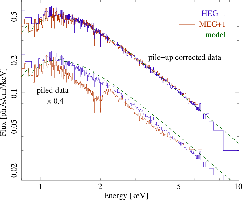
Figure 2.— Pile-up in the HEG (black curves) and MEG (gray curves) data: the lower spectra, which are shifted by a factor of 0.4, show the uncorrected data. The dashed line shows the model (free of pile-up). The MEG spectrum suffers from significant pile-up losses around 2 keV, where the highest count rate is obtained. The upper spectra show the pile-up corrected spectra. Note that we show ISIS’ (model independent) flux spectra only for illustration; simple_gpile(2) operates on the count rates predicted by a model.

The effect of pile-up is stronger in the MEG spectra than in the HEG spectra due to the lower dispersion and higher effective area of the MEG. The apparent flux reduction is most significant near 2 keV where the spectrometer has the largest efficiency and the highest count rates are obtained (see Figure 2). It can, however, excellently be modeled with simple_gpile2. When fitting a spectrum, there is always a strong correlation between the pile-up scale $\gamma$ and the corresponding flux normalization factor, e.g., the relative cross-calibration factor $c$ introduced in Section 3.2. The best-fit values for the pile-up scales $\gamma$ found in our data analysis (see Table 2) are only slightly larger than expected from Equation (3) (namely $\gamma_{0,{\rm MEG}\,\pm 1}=5.6\!\times\!10^{-2}\>$s Å and $\gamma_{0,{\rm HEG}\,\pm 1}=2.8\!\times\!10^{-2}\>$s Å), and the calibration factors $c$ are consistent with 1, except for the HEG$-1$ spectrum, for which both the largest $\gamma-\gamma_{0}$ and $c$ were found. Given the presence of the $\gamma$–$c$ correlation, we consider the latter to be a numerical artifact.

According to the simple_gpile2 model, the MEG+1 spectra suffer from $>$30 % pile-up for $6\,\mbox{\AA}\leq\lambda\leq 8.3\,$Å, peaking at $p_{\mathrm{MEG+1}}=45\,\%$ in the Si xiii f emission line at 6.74 Å. Except for some emission lines, among them the Fe K$\alpha$ line, the continuum pile-up fraction of the HEG spectra is below 17 %. For the HEG+1 spectrum, the reduction is less than 10 % outside the ranges $2.09\,\mbox{\AA}\leq\lambda\leq 4.08\,$Å and $6.05\,\mbox{\AA}\leq\lambda\leq 6.93\,$Å.

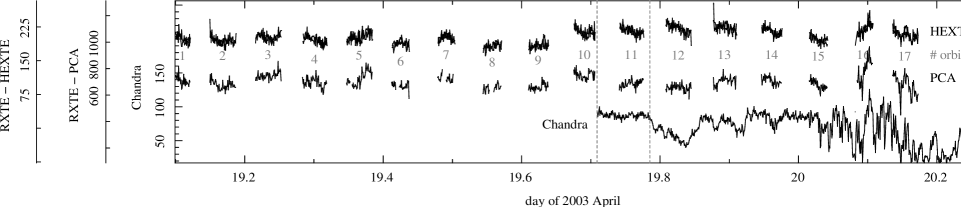
Figure 3.— Coverage of the simultaneous RXTE and Chandra observations. The plot shows the background-subtracted light curves with a time resolution of 64 s on a separate $y$ axis each. Top: RXTE-HEXTE (20–250 keV). The count rates have been corrected for the detector dead time. Center: RXTE-PCA (4–20 keV), normalized by the number of active PCUs. Bottom: Chandra-HETGS (0.5–12 keV, only first-order events; see Figure 4 for more details). The numbers label the RXTE orbits, vertical lines mark the first part of the nondip spectrum (see Section 3.1 and Figure 4), which completely covers RXTE orbit 11.

2.3. RXTE Observation

While Chandra’s HETGS provides a high spectral resolution, the energy range covered is rather limited. Within the framework of our RXTE monitoring campaign, the broadband spectrum of Cyg X-1 was measured regularly, i.e., at least biweekly, since 1998 (see Wilms et al. 2006, and references therein). The observation on 2004 April 19 was extended to provide hard X-ray data simultaneously with the Chandra observation. More than one day was covered by 17 RXTE orbits of $\sim$47 min good time, interrupted by $\sim$49 min intervals when Cyg X-1 was not observable due to Earth occultations or passages through the South Atlantic Anomaly (SAA), see Figure 3.

Data in the 4–20 keV range from the Proportional Counter Array (PCA; Jahoda et al. 1996) and in the 20–250 keV range from the High Energy X-Ray Timing Experiment (HEXTE; Gruber et al. 1996) were used. The data were extracted using HEASOFT 6.3.1, following standard data screening procedures as recommended by the RXTE Guest Observer Facility. Data were only used if taken more than 30 minutes away from the SAA. For the PCA, only data taken in the top layer of the proportional counter were included in the final spectrum, and no additional systematic error was added to the spectrum. During the observation, different sets of Proportional Counter Units (PCUs) were operative. During the 11th orbit, extensively used in this work, PCUs 1 and 4 were off.

3. Analysis

3.1. Light Curve

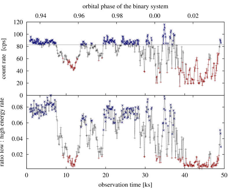
Figure 4.— Top: full 0.5–12 keV band Chandra light curve. Bottom: ratio of 0.7–1 keV band and 2.1–7.2 keV band count rates. Absorption dips – at first compact, then with complex substructure – show up with a reduced flux and spectral hardening. Count rates $>$82.7 cps define the nondip data (dark).

The Chandra observation covers a phase range between $\sim$0.93 and $\sim$0.03 in the 5.599829 d binary orbit (Gies et al. 2003, whose epoch is HJD $2451730.449\pm 0.008$). The top panel of Figure 4 shows the light curve of first-order events (MEG$\pm$1, HEG$\pm 1$) in the full band accessible with Chandra-HETGS. During several dip events, the flux is considerably reduced. The absorption dips distinguish themselves also by spectral hardening (the bottom panel of Figure 4). We extract a 16.1 ks nondip spectrum, which is the subject of this paper, from all times when the total count rate exceeds 82.7 cps; these are indicated by dark points in Figure 4. The analysis of dip spectra will be described in a subsequent paper.

The RXTE light curve shows considerable variability as well. Although the dips are more obviously detected with Chandra in the soft X-ray band, similar structures are also seen with RXTE-PCA or even -HEXTE, especially in the last RXTE orbits of these observations (Figure 3). We chose to infer the nondip broadband spectrum from the RXTE data taken during the 11th orbit, which was performed entirely during the first part of the nondip phase. Other parts are interrupted by dips, occultations, or have nonuniform PCU configuration.

3.2. Continuum Spectrum

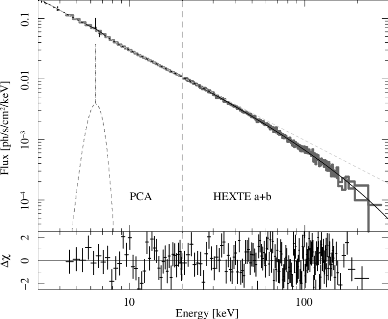
Figure 5.— RXTE 4–250 keV broadband continuum spectrum, as measured with PCA below 20 keV and above 20 keV with HEXTE, which can be described by a broken power-law with high-energy cutoff and a weak iron line, see Table 2. Due to the joint fit with Chandra, the Fe line consists of narrow and a broad component, see Figure 6. The HEXTE spectra shown are renormalized to match the PCA flux, as the absolute calibrations of these two instruments differ by $\sim$15%.

Table 2Fit Parameters of the Continuum Nondip Hard State Spectrum of Cyg X-1

		Fit to the	Joint Fit to Both the
Parameter	Unit	Chandra	Chandra and RXTE
		Spectra Only	Spectra
Photoabsorption
$N_{\mathrm{H}}$	10${}^{21}\>$cm-2	$3.52\pm 0.04$	$5.4\pm 0.4$
(Broken) power-law
$\Gamma_{1}$ (HETGS)		$1.51\pm 0.01$	$1.60\pm 0.01$
$\Gamma_{1}$ (PCA)		$\cdots$	$1.73\pm 0.01$
$E_{\mathrm{break}}$	keV	$\cdots$	$9.0^{+0.3}_{-1.5}$
$\Gamma_{2}$		$\cdots$	$1.50\pm 0.01$
norm	s${}^{-1}\>$cm${}^{-2}\>$keV-1	$1.15\pm 0.01$	$1.33\pm 0.03$
High-energy cutoff
$E_{\mathrm{cut}}$	keV	$\cdots$	$24^{+2}_{-3}$
$E_{\mathrm{fold}}$	keV	$\cdots$	$204\pm 9$
Disk black body
$A_{\mathrm{disk}}$ (Equation 6)	$10^{3}$	$\cdots$	$23^{+17}_{-12}$
$k\,T_{\mathrm{col}}$	keV	$\cdots$	$0.25^{+0.03}_{-0.02}$
Narrow iron K$\alpha$ line
$E_{0,\mathrm{narrow}}$	keV	$\cdots$	$6.4001^{+0.0004}_{-0.0092}$
$\sigma_{\mathrm{narrow}}$	eV (!)	$\cdots$	$<0.1$
$A_{\mathrm{narrow}}$	$10^{-3}\>$s${}^{-1}\>$cm-2	$\cdots$	$1.0\pm 0.3$
Broad iron K$\alpha$ line
$E_{0,\mathrm{broad}}$	keV	$\cdots$	6.4 (fixed)
$\sigma_{\mathrm{broad}}$	keV	$\cdots$	$0.6\pm 0.1$
$A_{\mathrm{broad}}$	$10^{-3}\>$s${}^{-1}\>$cm-2	$\cdots$	$4.3^{+2.7}_{-0.5}$
Relative flux calibration (constant factor)
$c_{\mathrm{MEG-1}}$		1 (fixed)	1 (fixed)
$c_{\mathrm{MEG+1}}$		$1.00\pm 0.01$	$0.99\pm 0.01$
$c_{\mathrm{HEG-1}}$		$1.04\pm 0.01$	$1.04\pm 0.01$
$c_{\mathrm{HEG+1}}$		$1.01\pm 0.01$	$1.02\pm 0.01$
$c_{\mathrm{PCA}}$		$\cdots$	$1.18\pm 0.03$
$c_{\mathrm{HEXTE}}$		$\cdots$	$1.03^{+0.02}_{-0.03}$
Pile-up scales
$\gamma_{\mathrm{MEG-1}}$	10${}^{-2}\>$s Å	$5.6\pm 0.1$	$5.6\pm 0.1$
$\gamma_{\mathrm{MEG+1}}$	10${}^{-2}\>$s Å	$6.0\pm 0.1$	$5.9\pm 0.1$
$\gamma_{\mathrm{HEG-1}}$	10${}^{-2}\>$s Å	$4.5\pm 0.3$	$4.6\pm 0.3$
$\gamma_{\mathrm{HEG+1}}$	10${}^{-2}\>$s Å	$3.5\pm 0.3$	$3.8\pm 0.3$
Fit-statistics
$\chi^{2}$		11745	12180
dof		11274$-$10	$11274^{b}+293^{b}-25^{c}$
$\chi^{2}_{\mathrm{red}}$		1.04	1.06
Absorbed flux (pile-up corrected)
$S_{\mathrm{0.5-10\,keV}}$	photons s-1 cm-2	1.4
$F_{\mathrm{0.5-10\,keV}}$	$10^{-9}$ erg s-1 cm-2	7.4
$S_{\mathrm{0.5-250\,keV}}$	photons s-1 cm-2	$\cdots$	1.8
$F_{\mathrm{0.5-250\,keV}}$	$10^{-9}$ erg s-1 cm-2	$\cdots$	24
Unabsorbed luminosity, assuming $d=2.5\,$kpc (Ninkov et al. 1987a)
$L_{\mathrm{0.5-10\,keV}}$	$10^{37}$ erg s-1	0.67	0.78
$L_{\mathrm{0.5-250\,keV}}$	$10^{37}$ erg s-1	$\cdots$	3.1

Notes. Error bars indicate 90% confidence intervals for one interesting parameter.

The broadband spectrum of Cyg X-1 in the hard state can be described by a broken power-law with exponential cutoff (Figure 5). Since the parameters of this phenomenological model are correlated with those of physical Comptonization models (see, e.g., Wilms et al. 2006, Fig. 11), we are justified in using the aforementioned simple continuum model for this paper focusing on the spectroscopy of the wind. We describe the whole 0.5–250 keV spectrum consistently with one broken power-law model, i.e., there is no need to fit the continuum locally.

Taking pile-up into account (Section 2.2), the nondip Chandra spectra alone can already be described quite well by a weakly absorbed, relatively flat power-law spectrum with a photon index $\Gamma_{1}=1.51\pm 0.01$ (Table 2). This result is consistent with the fact that the break energy of the broadband broken power-law spectrum is found at $E_{\mathrm{break}}=9\,$keV, i.e., the Chandra data are virtually entirely in the regime of the (steeper) photon index $\Gamma_{1}$. The onset of the exponential cutoff (with folding energy $E_{\mathrm{fold}}$) is at $E_{\mathrm{cut}}=24\,$keV and thus also well above the spectral range of Chandra. As it is known that there are cross-calibration uncertainties between Chandra and RXTE (Kirsch et al. 2005), we use constant factors $c_{i}$ for the relative flux calibration of every spectrum and also separate parameters $\Gamma_{1}$(HETGS) and $\Gamma_{1}$(PCA), for which we find similar values within the joint model (see Table 2). In order to describe a weak soft excess, we add a thermal disk component, which accounts for $\sim$9 % of the unabsorbed 0.5–10 keV flux. The disk has a color temperature of $kT_{\mathrm{col}}=0.25\,$keV; similar to that found by Makishima et al. (2008) and Bałucińska-Church et al. (1995), who described the soft excess with a $kT=0.13\pm 0.02$ keV blackbody only, but the temperature $T_{\mathrm{col}}$ may be too high by a factor $f\gtrsim 1.7$ (Shimura & Takahara 1995). The norm parameter of the diskbb model is

$$A_{\mathrm{disk}}\;\;=\;\;\mathtt{diskbb\ .\ norm}\;\;=\;\;\left(\frac{R_{\mathrm{col}}/\mathrm{km}}{d/10\,\mathrm{kpc}}\right)^{2}\cdot\>\cos\,\theta\;\;,$$ (6)

where $d$ is the distance and $\theta$ is the inclination of the disk, which can deviate from the orbital inclination $i\approx 35^{\circ}$ (Herrero et al. 1995) as the disk may be precessing with a tilt $\delta\approx 37^{\circ}$ (Brocksopp et al. 1999). $R_{\mathrm{col}}$ is related to the inner radius of the disk, $R_{\mathrm{in}}=\eta\,g(i)\,f^{2}\cdot R_{\mathrm{col}}$ (with $\eta\approx 0.6-0.7$ and $g(i)\approx 0.7-0.8$; Merloni et al. 2000). In spite of these uncertainties and the large statistical error of $A_{\mathrm{disk}}$ (more than 50 %), the inner disk radius can be estimated to $1.5\,R_{\mathrm{S}}\lesssim R_{\mathrm{in}}\lesssim 10\,R_{\mathrm{S}}$ if a distance $d\approx 2.5\,$kpc (Ninkov et al. 1987a) and a Schwarzschild radius $R_{\mathrm{S}}\approx 30\,$km (Herrero et al. 1995) are assumed. Thus, the disk is consistent with extending close to the innermost stable circular orbit (ISCO).

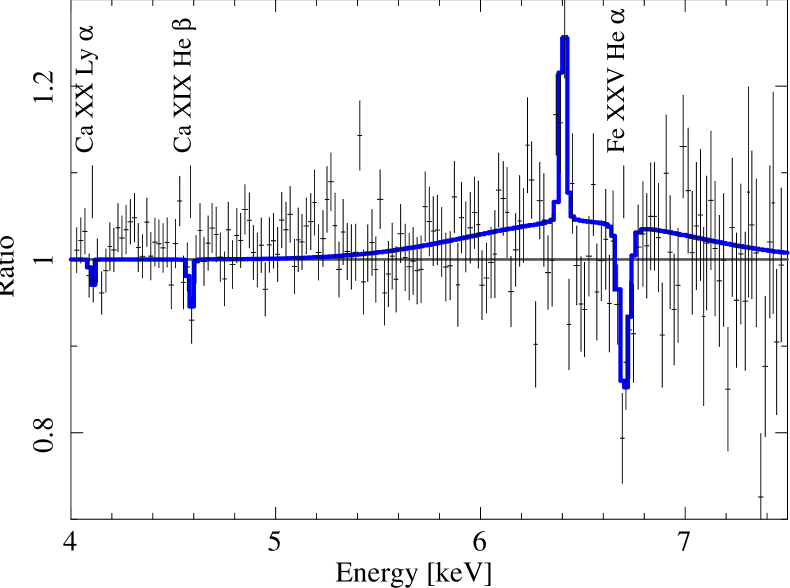
Figure 6.— Chandra-HEG spectrum in the Fe line region. The model includes both the narrow and the broad K$\alpha$ emission line, the latter as required by the simultaneous RXTE-PCA data, and the Fe xxv and Ca xix/xx absorption lines.

The good S/N afforded by the RXTE-PCA data clearly reveals an iron fluorescence K$\alpha$ line. While the instrumental response of the proportional counters does not allow for a resolution of the line profile details, i.e., whether it is narrow or relativistically broadened, the Chandra-HEG spectra (Figure 6) do resolve a strong narrow component at 6.4 keV. Nevertheless, since the integrated flux of the Chandra measured line is insufficient to account for all of the PCA residuals in this region, we include an additional broad feature to our modeling, which is also compatible with the Chandra spectrum. Given the relatively low S/N at these energies, we do not model the broad iron line with a proper physical model such as a relativistically broadened line, but use a Gaussian with its energy fixed at 6.4 keV, as the latter is hardly constrained by the data. These results illustrate the synergy of the simultaneous observation with complementary instruments, as the combination of narrow and broad line could only be revealed by the analysis with a joint model.

Our global model for the continuum spectrum now enables us to address the features of the high-resolution Chandra spectra, which is the topic in the remainder of this section.

3.3. Neutral Absorption

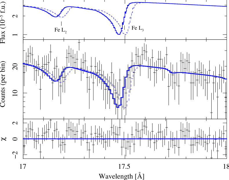
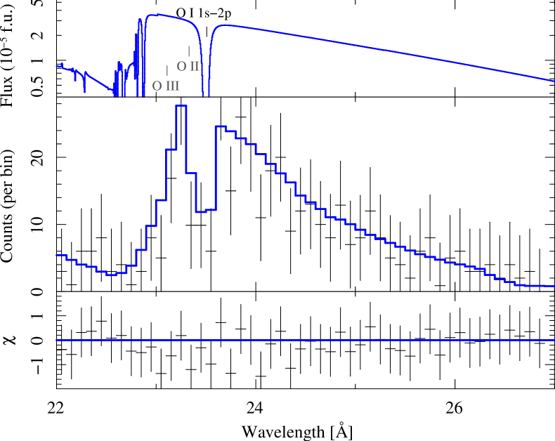
Figure 7.— Spectral region around the Fe L-edges. The top panel shows the model flux in units of $10^{-5}$ ph. s^-1 cm^-2 Å^-1 (solid line). The dashed lines describe the unshifted model, see the text. The second panel shows the count rate of all the four HETGS spectra (MEG$\pm 1$, HEG$\pm 1$), which have been combined with a resolution of 10 mÅ, and the folded model. The bottom panel displays the residuals $\chi=($data–model)/error.

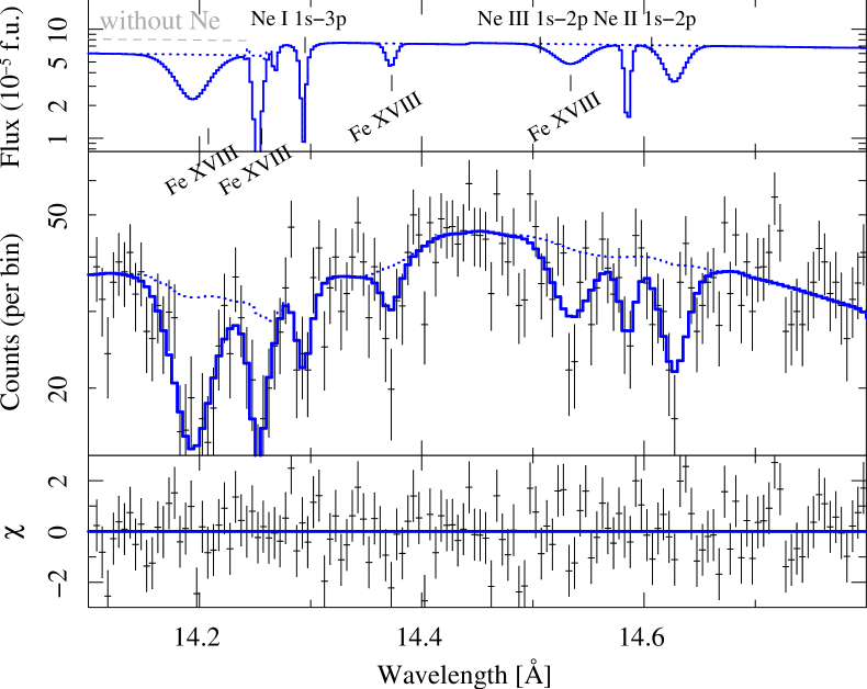
Figure 8.— Same as in Figure 9, but for the spectral region around the O K-edge. Both MEG$\pm 1$ spectra have been combined with a resolution of 0.1 Å.

Figure 9.— Same as in Figure 9, but for the spectral region around the Ne K-edge. All spectra have been combined with a resolution of 5 mÅ. The dotted lines show the absorbed continuum model without additional absorption lines. The light dashed line shows the model without the absorption of Ne.

Absorbing columns can be measured most accurately from the discrete edges in high-resolution spectra at the ionization thresholds. We detect the most prominent L-shell absorption edge of iron and the K-shell absorption edges of oxygen and neon. Juett et al. (2004, 2006a) have inferred the fine structure at those edges from earlier Chandra-HETGS observations of Cyg X-1 and other bright X-ray binaries: the Fe L₂ and L₃ edges, due to the ionization of a 2p_1/2 or a 2p_3/2 electron, respectively, are separately detectable at 17.2 Å and 17.5 Å. The O K-edge at 22.8 Å is accompanied by (1s$\rightarrow$2p) K$\alpha$ and higher ($1$s$\rightarrow n$p) resonance absorption lines. The K$\alpha$ line occurs at 23.5 Å for neutral O i and at lower wavelengths for ionized oxygen. In the case of neon, neutral atoms have closed L-shells, such that Ne i only shows a (1s$\rightarrow$3p) K$\beta$ absorption line close to the K-edge at 14.3 Å, while ionized neon also shows K$\alpha$ absorption lines, e.g., Ne ii at 14.6 Å and Ne iii at 14.5 Å. Improved modeling of the neutral absorption that takes these features into account has recently been included in the photoabsorption model tbnew (Juett et al. 2006b), an extension of the commonly used tbvarabs model (Wilms et al. 2000).

Table 3Column Density $N$ and Abundance $A=N/N_{\mathrm{H}}$ of Neutral Absorbers Detected Along the Line of Sight Toward Cyg X-1

					Analysis by
		This work			Schulz et al. (2002)	Juett et al. (2004, 2006a)
					———————	——————————————————————
		ObsID 3814			ObsID 107	ObsID 107	ObsID 3407	ObsID 3724
		($L_{0.5-10\,\mathrm{kev}}=0.7\!\times\!10^{37}\,$erg s-1)			($L_{0.5-10\,\mathrm{kev}}=1.6\!\times\!10^{37}\,$erg s-1)		($3.1\!\times\!10^{37}\,$erg s-1)	(soft state)
		————————————————————			———————	—————	—————	—————
Element	$12+\log\,A_{\mathrm{element}}^{\mathrm{ISM}}$	$N_{\mathrm{element}}/N_{\mathrm{Fe}}$	$A_{\mathrm{element}}/A_{\mathrm{element}}^{\mathrm{ISM}}$	$N_{\mathrm{element}}$	$N_{\mathrm{element}}$	$N_{\mathrm{element}}$	${N_{\mathrm{element}}}^{e}$	${N_{\mathrm{element}}}^{e}$
				($10^{17}\,$cm-2)	($10^{17}\,$cm-2)	($10^{17}\,$cm-2)	($10^{17}\,$cm-2)	($10^{17}\,$cm-2)
O	8.69	$15.4\pm 0.3$	$1.45\pm 0.01$	$38.1^{+0.4}_{-0.3}$	$39.2\pm 2.3$	$63\pm 14$	$24\pm 3$	$29\pm 3$
Ne	7.94	$3.91\pm 0.18$	$2.07^{+0.04}_{-0.03}$	$9.6\pm 0.2$	$9.43\pm 0.32$	$7.1\pm 1.0$	$7.4^{+0.7}_{-0.3}$	$8.6\pm 0.7$
Na	6.16	$1.26\pm 0.15$	$40\pm 2$	$3.1\pm 0.2$	$\cdots$	$\cdots$	$\cdots$	$\cdots$
Mg	7.40	$2.16\pm 0.13$	$4.0\pm 0.1$	$5.3\pm 0.2$	$3.7\pm 1.3$	$\cdots$	$\cdots$	$\cdots$
Al	6.33	$<0.13$	$<1.8$	$<0.2$	$\cdots$	$\cdots$	$\cdots$	$\cdots$
Si	7.27	$1.45\pm 0.17$	$3.8\pm 0.3$	$3.8\pm 0.3$	$2.3\pm 1.8$	$\cdots$	$\cdots$	$\cdots$
S	7.09	$0.6\pm 0.2$	$2.4^{+0.5}_{-0.3}$	$1.6^{+0.3}_{-0.2}$	$\cdots$	$\cdots$	$\cdots$	$\cdots$
Ar	6.41	$<0.06$	$<1.0$	$<0.1$	$\cdots$	$\cdots$	$\cdots$	$\cdots$
Ca	6.20	$<0.05$	$<1.3$	$<0.1$	$\cdots$	$\cdots$	$\cdots$	$\cdots$
Cr	5.51	$<0.18$	$1.3^{+2.7}_{-1.3}$	$0.02^{+0.05}_{-0.02}$	$\cdots$	$\cdots$	$\cdots$	$\cdots$
Fe	7.43	1	$1.75\pm 0.03$	$2.52\pm 0.04$	$1.5\pm 0.1$	$1.47^{+0.25}_{-0.19}$	$1.06^{+0.07}_{-0.11}$	$0.96\pm 0.09$

Notes.

As part of the spectral model for the whole continuum, the tbnew model can be used to describe the absorption edges detected with the Chandra observation of Cyg X-1 discussed in this paper. Figure 9 shows the Fe L-edges requiring a blueshift by $\Delta\lambda/\lambda_{0}\cdot c=(540\pm 230)\>$km s^-1 of the tbnew model, which relies on the cross sections of metallic iron measured by Kortright & Kim (2000). Unlike Schulz et al. (2002), Miller et al. (2005) and Juett et al. (2006a) have also found that the Fe L₃ edge requires a small shift; their mean position of maximum optical depth is $\lambda_{\mathrm{Fe\>L_{3}}}=17.498\,$Å, but our value $\lambda_{\mathrm{Fe\>L_{3}}}=(17.469\pm 0.014)\,$Å is still lower. The shift could be caused by the Doppler effect due to a moving absorber, by a modified ionization threshold due to chemical bonds, or ionization of the iron atoms (van Aken & Liebscher 2002). In an analysis of the Cyg X-1 high/soft and low/hard state, focused on this spectral region, J. Lee et al. (2008, in preparation) find that the Fe L-edges here can likely be modeled by a heterogeneous combination of gas and condensed matter of iron in combination with oxygen local to the source environment. If, as suggested by these authors, the magnitude of the shift is due to molecules and/or dust, this shift is one identifying signature of the composition and charge state of the condensed state material. Such direct Chandra X-ray spectroscopic detection of dust via its associated edge structure was first suggested for observations of the Fe L-edge in the active galactic nucleus MCG$-$6-30-15 (Lee et al. 2001) and for the observations of the Si K-edge in the microquasar GRS 1915+105 (Lee et al. 2002). The latter study associated the observed Si K-edge structure with SiO₂, although the origin – source environment or Chandra CCD gate structure – was unclear in this case.

The blueshift of $(100\pm 130)\>$km s^-1 which has been determined for all other absorption edges is consistent with zero. The O K-edge can only be seen in the MEG spectra after heavy rebinning (Figure 9). Nevertheless, the K$\alpha$ resonance absorption line of O i is clearly detected. The region around the Ne edge (Figure 9) is dominated by Fe xviii absorption lines, possibly blending with the K$\alpha$ absorption lines of Ne ii and Ne iii. No other strong edges are clearly visible in the spectrum. The Na K-edge (at 11.5 Å; Verner & Yakovlev 1995) blends with an absorption line due to the 2s$\rightarrow$3p excitation of Fe xxii. The Mg K-edge (at 9.5 Å) blends with the Ne x Ly $\delta$ absorption line. The Si K-edge (at 6.7 Å) is strongly affected by pile-up and blends with the Mg xii Ly $\beta$ absorption line. The S K-edge (at 5.0 Å) is relatively weak. Neutral absorption from these elements is nevertheless required within the tbnew model.

The results for the individual abundances, $A_{i}=N_{i}/N_{\mathrm{H}}$, and resulting column densities, $N_{i}$, are presented in Table 3. The alpha process elements O, Ne, Mg, Si, and S are overabundant with respect to the interstellar medium (ISM) abundances as summarized by Wilms et al. (2000) and therefore suggest an origin in the system itself. The total column densities are also compared with the values obtained by Schulz et al. (2002) and Juett et al. (2004, 2006a) from other Chandra observations of Cyg X-1. Table 3 includes the corresponding source luminosities if they are reported in the literature (see also Section 4.4). The X-ray flux was highest during the soft state observation with the observation identification (ObsID) 3724. The column densities confirm the conjecture of Juett et al. (2004) that a higher (soft) X-ray flux ionizes material local to the Cyg X-1 system and reduces the neutral abundances.

The inferred hydrogen column density $N_{\mathrm{H}}$ (see Table 2) is in very good agreement with that from ASCA observations during the soft state in 1996, namely $N_{\mathrm{H}}=(5.3\pm 0.2)\times 10^{21}\,$cm^-2 (Dotani et al. 1997), and also with $N_{\mathrm{H}}=6.2\!\times\!10^{21}\>\mathrm{cm}^{-2}$ obtained from two other different Chandra observations (Schulz et al. 2002; Miller et al. 2002, see also Section 4.4). We note that the large column density toward Cyg X-1 found by many online tools, $(7.2-7.8)\times\!10^{21}\,$cm^-2, is obtained from a coarse grid – with (0.675 deg)² pixel size – of $N_{\mathrm{H}}$ measurements at 21 cm (Kalberla et al. 2005), which does not resolve the strong variations of $N_{\mathrm{H}}$ in the region around Cyg X-1 (Russell et al. 2007).

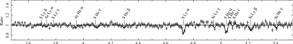
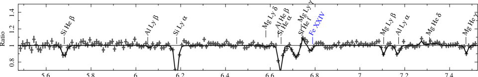
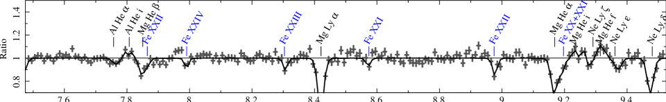
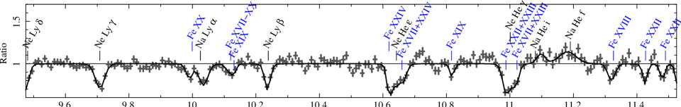
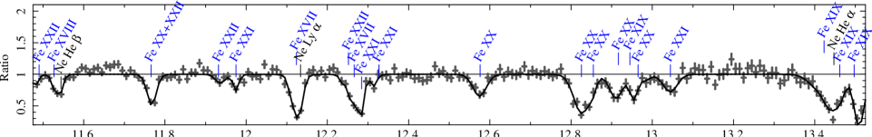
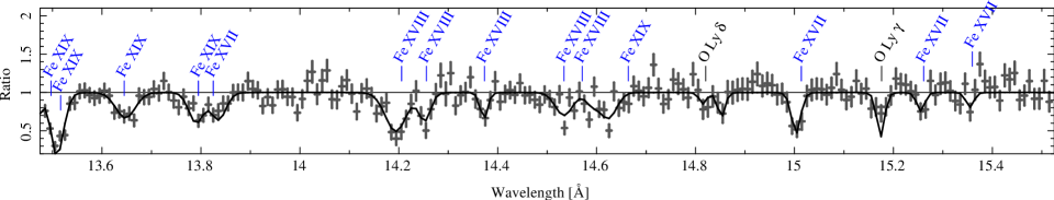
Figure 10.— Chandra (nondip) spectrum of Cyg X-1, shown as ratio of data and continuum model (Table 2). For visual clarity, the data have been rebinned to a common resolution of 10 mÅ, and all MEG$\pm 1$ and HEG$\pm 1$ spectra have been combined. The Gaussian line fits and identifications are shown as well. (The labels mark the lines’ rest wavelengths.) Iron L-shell transitions (lines of Fe $\small<$xxv) are shown in blue in the online journal.

3.4. Absorption Lines of H- and He-Like Ions

Table 4Overview on the Detected Lines from H- and He-Like Ions: Theoretical Rest Wavelengths in Å

Transition		O	Ne	Na	Mg	Al	Si	S	Ar	Ca	Fe	Ni
Hydrogen-like (1 electron)		viii	x	xi	xii	xiii	xiv	xvi	xviii	xx	xxvi	xxviii
Ly $\alpha$	1s$\>(^{2}\mathrm{S}_{1/2})\rightarrow 2$p$\>(^{2}\mathrm{P}_{3/2,1/2})$	18.97	12.13	10.03	8.42	7.17	6.18	4.73	3.73	3.02	(1.78)	1.53
Ly $\beta$	1s$\>(^{2}\mathrm{S}_{1/2})\rightarrow 3$p$\>(^{2}\mathrm{P}_{3/2,1/2})$	16.01	10.24	8.46	7.11	6.05	5.22	3.99	3.15	(2.55)	1.50	1.29
Ly $\gamma$	1s$\>(^{2}\mathrm{S}_{1/2})\rightarrow 4$p$\>(^{2}\mathrm{P}_{3/2,1/2})$	15.18	9.71	8.02	(6.74)	5.74	4.95	3.78	2.99	2.42	1.43	1.23
Ly $\delta$	1s$\>(^{2}\mathrm{S}_{1/2})\rightarrow 5$p$\>(^{2}\mathrm{P}_{3/2,1/2})$	14.82	9.48	7.83	6.58	(5.60)	(4.83)	3.70	(2.92)	(2.36)	(1.39)	(1.20)
Ly $\epsilon$	1s$\>(^{2}\mathrm{S}_{1/2})\rightarrow 6$p$\>(^{2}\mathrm{P}_{3/2,1/2})$	(14.63)	9.36	( 7.73)	6.50	(5.53)	(4.77)	(3.65)	(2.88)	(2.33)	(1.37)
Ly $\zeta$	1s$\>(^{2}\mathrm{S}_{1/2})\rightarrow 7$p$\>(^{2}\mathrm{P}_{3/2,1/2})$	(14.52)	9.29	( 7.68)	6.45	(5.49)	(4.73)	(3.62)	(2.86)	(2.31)	(1.36)
Ly $\eta$	1s$\>(^{2}\mathrm{S}_{1/2})\rightarrow 8$p$\>(^{2}\mathrm{P}_{3/2,1/2})$	(14.45)	9.25	( 7.64)	(6.42)	(5.47)	(4.71)	(3.60)	(2.85)	(2.30)	(1.36)
Ly $\theta$	1s$\>(^{2}\mathrm{S}_{1/2})\rightarrow 9$p$\>(^{2}\mathrm{P}_{3/2,1/2})$	(14.41)	( 9.22)	( 7.61)	(6.40)	(5.45)	(4.70)	(3.59)	(2.84)	(2.29)	(1.35)
$\cdots$
limit	$1$s$\>(^{2}\mathrm{S}_{1/2})\rightarrow\infty$	(14.23)	( 9.10)	( 7.52)	6.32	5.38	(4.64)	(3.55)	(2.80)	(2.27)	1.34	(1.15)
Transition		O	Ne	Na	Mg	Al	Si	S	Ar	Ca	Fe	Ni
Helium-like (2 electrons)		vii	ix	x	xi	xii	xiii	xv	xvii	xix	xxv	xxvii
f [em.]	$1$s${}^{2}\>(^{1}\mathrm{S}_{0})\leftarrow 1$s$2$s$\>(^{3}\mathrm{S}_{1})$	22.10	(13.70)	11.19	9.31	7.87	6.74	5.10	(3.99)	(3.21)	(1.87)
i [em.]	$1$s${}^{2}\>(^{1}\mathrm{S}_{0})\leftarrow 1$s$2$p$\>(^{3}\mathrm{P}_{1,2})$	21.80	(13.55)	11.08	9.23	7.81	(6.69)	5.07	3.97	3.19	(1.86)	1.60
r $\equiv$ He $\alpha$	$1$s${}^{2}\>(^{1}\mathrm{S}_{0})\rightarrow 1$s$2$p$\>(^{1}\mathrm{P}_{1})$	21.60	13.45	11.00	9.17	7.76	6.65	5.04	3.95	3.18	1.85	1.59
He $\beta$	$1$s${}^{2}\>(^{1}\mathrm{S}_{0})\rightarrow 1$s$3$p$\>(^{1}\mathrm{P}_{1})$	18.63	11.54	9.43	7.85	6.64	5.68	4.30	3.37	2.71	1.57	(1.35)
He $\gamma$	$1$s${}^{2}\>(^{1}\mathrm{S}_{0})\rightarrow 1$s$4$p$\>(^{1}\mathrm{P}_{1})$	(17.77)	11.00	8.98	7.47	6.31	5.40	4.09	3.20	(2.57)	1.50	(1.28)
He $\delta$	$1$s${}^{2}\>(^{1}\mathrm{S}_{0})\rightarrow 1$s$5$p$\>(^{1}\mathrm{P}_{1})$	(17.40)	10.77	8.79	7.31	(6.18)	(5.29)	4.00	(3.13)	(2.51)	1.46	(1.25)
He $\epsilon$	$1$s${}^{2}\>(^{1}\mathrm{S}_{0})\rightarrow 1$s$6$p$\>(^{1}\mathrm{P}_{1})$	(17.20)	10.64	( 8.69)	(7.22)	(6.10)	5.22	3.95	(3.10)
He $\zeta$	$1$s${}^{2}\>(^{1}\mathrm{S}_{0})\rightarrow 1$s$7$p$\>(^{1}\mathrm{P}_{1})$	(17.09)	10.56	( 8.63)	(7.17)	(6.06)	(5.19)	(3.92)
He $\eta$	$1$s${}^{2}\>(^{1}\mathrm{S}_{0})\rightarrow 1$s$8$p$\>(^{1}\mathrm{P}_{1})$	(17.01)	(10.51)	( 8.59)	(7.14)	(6.03)	(5.16)	(3.90)
$\cdots$
limit	$1$s${}^{2}\>(^{1}\mathrm{S}_{0})\rightarrow 1$s$\>\infty$	16.77	10.37	8.46	(7.04)	5.94	5.09	(3.85)	(3.01)	2.42	1.40	(1.20)

Notes. Lines with (wavelengths in parentheses) are not detected in our Chandra-HETGS observation of Cyg X-1, while lines indicated with bold wavelengths are clearly detected and those with underlined wavelengths are detected as two components. The wavelengths of the lines are taken from the CXC atomic database atomdb and the table of Verner et al. (1996), those of the series limits (= K-ionization thresholds) are from Verner & Yakovlev (1995).

Table 5Results from the Detected Absorption Lines from H- and He-Like Ions: Velocity Shifts $v=(\lambda-\lambda_{0})/\lambda_{0}\cdot c$ in $\rm km\,s^{-1}$

	O	Ne	Na	Mg	Al	Si	S	Ar	Ca	Fe
H-like	viii	x	xi	xii	xiii	xiv	xvi	xviii	xx	xxvi
Ly $\alpha$	$-718^{+1716}_{-281}$	$-128^{+35}_{-27}$	$284^{+81}_{-81}$	$-34^{+26}_{-34}$	$-171^{+88}_{-104}$	$-60^{+32}_{-33}$	$-43^{+114}_{-95}$	$-322^{+712}_{-617}$	$164^{+838}_{-402}$	$\cdots$
Ly $\beta$	$-90^{+187}_{-185}$	$-72^{+50}_{-47}$	$\cdots$	$17^{+27}_{-73}$	$344^{+431}_{-448}$	$75^{+263}_{-238}$	$\cdots$	$-750^{+710}_{-451}$	$\cdots$	$\cdots$
Ly $\gamma$	$-39^{+85}_{-81}$	$7^{+64}_{-64}$	$\cdots$	$\cdots$	$\cdots$	$308^{+333}_{-193}$	$-347^{+393}_{-399}$	$\cdots$	$\cdots$	$\cdots$
Ly $\delta$	$-109^{+1109}_{-198}$	$-192^{+46}_{-46}$	$\cdots$	$3^{+922}_{-1401}$	$\cdots$	$\cdots$	$420^{+536}_{-489}$	$\cdots$	$\cdots$	$\cdots$
Ly $\epsilon$	$\cdots$	$288^{+213}_{-177}$	$\cdots$	$\cdots$	$\cdots$	$\cdots$	$\cdots$	$\cdots$	$\cdots$	$\cdots$
Ly series	$-41^{+67}_{-72}$	$-97^{+28}_{-20}$	$207^{+104}_{-101}$	$-38^{+27}_{-28}$	$-183^{+140}_{-117}$	$-54^{+33}_{-32}$	$-90^{+74}_{-73}$	$-327^{+41}_{-128}$	$\cdots$	$\cdots$
	O	Ne	Na	Mg	Al	Si	S	Ar	Ca	Fe
He-like	vii	ix	x	xi	xii	xiii	xv	xvii	xix	xxv
He $\alpha$	$\cdots$	$-203^{+85}_{-91}$	$\cdots$	$-71^{+35}_{-49}$	$286^{+187}_{-574}$	$-30^{+23}_{-46}$	$84^{+127}_{-138}$	$-142^{+250}_{-233}$	$1124^{+98}_{-1069}$	$-116^{+501}_{-531}$
He $\beta$	$507^{+492}_{-1020}$	$-36^{+47}_{-0}$	$\cdots$	$-65^{+44}_{-0}$	$59^{+54}_{-46}$	$18^{+165}_{-195}$	$609^{+785}_{-1556}$	$72^{+440}_{-306}$	$-74^{+616}_{-422}$	$\cdots$
He $\gamma$	$\cdots$	$-507^{+106}_{-123}$	$\cdots$	$77^{+81}_{-71}$	$\cdots$	$-19^{+320}_{-234}$	$702^{+478}_{-658}$	$655^{+283}_{-470}$	$\cdots$	$\cdots$
He $\delta$	$\cdots$	$\cdots$	$\cdots$	$\cdots$	$\cdots$	$\cdots$	$\cdots$	$\cdots$	$\cdots$	$\cdots$
He $\epsilon$	$\cdots$	$-93^{+54}_{-59}$	$\cdots$	$\cdots$	$\cdots$	$\cdots$	$\cdots$	$\cdots$	$\cdots$	$\cdots$
He series	$-291\pm({>}1000)$	$-158^{+35}_{-56}$	$\cdots$	$-72^{+25}_{-28}$	$135^{+205}_{-234}$	$-86^{+26}_{-41}$	$47^{+37}_{-52}$	$2^{+8}_{-12}$	$\cdots$	$-21^{+0}_{-379}$

Notes. A negative velocity indicates a blue shift, due to the absorbing material moving toward the observer. Rows labeled with “Ly/He series” show the results from modeling the complete absorption line series of the corresponding ion at once with a single physical model (Section 3.5).

Table 6Results from the Detected Absorption Lines from H- and He-Like Ions: Column Densities in $10^{16}\,\rm cm^{-2}$

	O	Ne	Na	Mg	Al	Si	S	Ar	Ca	Fe
H-like	viii	x	xi	xii	xiii	xiv	xvi	xviii	xx	xxvi
Ly $\alpha$	$3^{+3}_{-1}$	$3.5^{+0.2}_{-0.3}$	$\cdots$	$5.2^{+0.2}_{-0.3}$	$1.8\pm 0.5$	$7.1^{+0.3}_{-0.4}$	$5.0^{+0.6}_{-1.1}$	$2.2^{+1.2}_{-1.8}$	$2\pm 2$	$\cdots$
Ly $\beta$	$15^{+3}_{-5}$	$10.8^{+1.2}_{-1.3}$	$\cdots$	$8.0^{+1.6}_{-1.8}$	$3^{+3}_{-2}$	$18^{+5}_{-6}$	$\cdots$	$7^{+9}_{-7}$	$\cdots$	$\cdots$
Ly $\gamma$	$20^{+5}_{-8}$	$51^{+5}_{-4}$	$\cdots$	$\cdots$	$\cdots$	$19\pm 13$	$18^{+19}_{-15}$	$\cdots$	$\cdots$	$\cdots$
Ly $\delta$	$11^{+13}_{-20}$	$82^{+9}_{-7}$	$\cdots$	$8^{+18}_{-8}$	$\cdots$	$\cdots$	$29^{+34}_{-29}$	$\cdots$	$\cdots$	$\cdots$
Ly series	$36^{+18}_{-12}$	$42^{+10}_{-4}$	$2.3^{+0.4}_{-0.5}$	$7.2\pm 0.6$	$1.4\pm 0.5$	$10.1\pm 0.8$	$15^{+12}_{-5}$	$11^{+1}_{-6}$	$\cdots$	$\cdots$
	O	Ne	Na	Mg	Al	Si	S	Ar	Ca	Fe
He-like	vii	ix	x	xi	xii	xiii	xv	xvii	xix	xxv
He $\alpha$	$\cdots$	$1.5\pm 0.2$	$\cdots$	$1.57^{+0.13}_{-0.15}$	$0.5^{+0.4}_{-0.1}$	$1.94^{+0.11}_{-0.18}$	$2.3^{+0.4}_{-0.5}$	$1.3\pm 0.6$	$1.0^{+0.9}_{-0.8}$	$15^{+3}_{-4}$
He $\beta$	$4^{+3}_{-6}$	$2.8^{+0.8}_{-0.4}$	$\cdots$	$5.6\pm 0.9$	$3.8^{+1.2}_{-0.6}$	$9^{+2}_{-3}$	$16^{+6}_{-9}$	$4\pm 4$	$11^{+5}_{-7}$	$\cdots$
He $\gamma$	$\cdots$	$3.0\pm 1.5$	$\cdots$	$8\pm 2$	$\cdots$	$8^{+5}_{-6}$	$23^{+11}_{-14}$	$21^{+11}_{-10}$	$\cdots$	$\cdots$
He series	$0^{+4}_{-0}$	$6.3^{+1.3}_{-1.6}$	$\cdots$	$5^{+2}_{-1}$	$0.8^{+0.2}_{-0.4}$	$12\pm 3$	$15^{+2}_{-3}$	$8^{+1}_{-4}$	$\cdots$	$146^{+80}_{-0}$

Notes. The column densities for the single lines have been calculated using Equation (11), assuming that the line is on the linear part of the curve of growth, which underestimates the column density for saturated lines. Rows labeled with “Ly/He series” show the results from modeling complete absorption line series (Section 3.5).

The high-resolution spectra reveal a large number of absorption lines of highly ionized ions. The 1.5–15 Å range is shown in Figure 10 as the ratio between the data and the continuum-model. As the line profiles are not fully resolved, we model each line $l$ with a Gaussian profile $G_{l}$. In terms of the continuum flux model, $F_{\mathrm{cont}}$, the global model reads

$$F(\lambda)\;\;=\;\;\mathrm{e}^{-\tau(\lambda)}\;\cdot\;F_{\mathrm{cont}}(\lambda)\;\;=\;\;\left[1+\sum_{l}G_{l}(\lambda)\right]\;\cdot\;F_{\mathrm{cont}}(\lambda)\;\;.$$ (7)

From a Gaussian’s centroid wavelength $\lambda$ and the rest wavelength $\lambda_{0}$ of the identified line, the radial velocity

$$v\;\;=\;\;(\lambda-\lambda_{0})/\lambda_{0}\cdot c$$ (8)

of the corresponding absorber can be inferred. With the definition in Equation (7), the norm of $G_{l}$ is just the equivalent width:

$$W_{\lambda,l}\;\;:=\;\;\int\!\!\left[1-F_{l}(\lambda)/F_{\mathrm{cont}}(\lambda)\right]\;\mathrm{d}\lambda\;\;=\;\;\int\!\!G_{l}(\lambda)\;\mathrm{d}\lambda$$ (9)

$W_{\lambda,l}$ is related to the absorber’s column density, as a bound–bound transition $i\rightarrow j$ (with the rest frequency $\nu_{0}$ and oscillator strength $f_{ij}$) in an absorbing plasma with column density $N_{i}$ creates the following line profile (see Mihalas 1978, Section9-2):

$$\mathrm{e}^{-\tau(\nu)}\;\;=\;\;\exp\left\{-N_{i}\>\frac{f_{ij}\,\sqrt{\pi}\,e^{2}}{m_{\mathrm{e}}\,c\,\Delta\nu_{\mathrm{D}}}\;H\!\left({\frac{\Gamma}{4\pi\>\Delta\nu_{\mathrm{D}}}},\;{\frac{\nu-\nu_{0}}{\Delta\nu_{\mathrm{D}}}}\right)\right\}$$ (10)

Assuming pure radiation damping, the damping constant $\Gamma$ equals the Einstein coefficient $A_{ji}$. The Doppler broadening $\Delta\nu_{\mathrm{D}}=\nu_{0}\cdot\xi_{0}/c$ is given by ${\xi_{0}}^{2}\>=\>{2kT}/{m_{\mathrm{ion}}}+v_{\mathrm{turb}}^{2}$, i.e., is due to the thermal and turbulent velocities of the plasma. For optically thin lines (with $\tau(\nu)\ll 1$), the equivalent width is independent of $\Delta\nu_{\mathrm{D}}$, such that the absorbing column density can be inferred (Spitzer 1978, Eq. 3-48; Mihalas 1978, §10-3):

$$N_{i}\;=\;\frac{m\,c^{2}\cdot W_{\lambda}}{\pi\,e^{2}\cdot f_{ij}\,\lambda_{0}^{2}}\;\;=\;\;\frac{1.13\!\times\!10^{17}\>\mathrm{cm}^{-2}}{f_{ij}}\cdot\left(\frac{\lambda_{0}}{\mbox{\AA}}\right)^{\!\!\!\!-2}\!\!\!\!\cdot\left(\frac{W_{\lambda}}{\mbox{m\AA}}\right)$$ (11)

If the lines are, however, saturated, $W_{\lambda}$ depends on $\Delta\nu_{\mathrm{D}}$ as well, and one has to construct the full “curve of growth” with several lines from a common ground state $i$ in order to constrain $N_{i}$ (see, e.g., Kotani et al. 2000).

We have therefore performed a systematic analysis of absorption line series: H-like ions are detected by their $1\mathrm{s}\rightarrow n\,\mathrm{p}$ Lyman series and He-like ions by their $1\mathrm{s}^{2}\rightarrow 1\mathrm{s}\>n\,\mathrm{p}$ resonance absorption series, see Table 4. For those lines that are clearly detected and not obviously affected by blends, the measured velocity shifts (Equation 8) are shown in Table 5. Most of the lines are detected at rather low projected velocity ($|v|<$200 km s^-1). Note that the systemic velocity of Cyg X-1/HDE 226868 is $(-7.0\pm 0.5)$ km s^-1 (Gies et al. 2003), and that the radial velocity of both the supergiant and the black hole vanishes at orbital phase $\phi_{\mathrm{orb}}=0$, while the radial component of the focused stream should be maximal (likely to be up to 720 km s^-1, see Section 4.1). The column densities in Table 6 are calculated using Equation (11), assuming that the line is on the linear part of the curve of growth. As the strongest lines are, however, often saturated, Equation (11) predicts too small column densities from them. For weak lines, however, the equivalent width is most likely to be overestimated such that the quoted values may rather be upper limits. The properties of the lines (Einstein $A$-coefficients and quantum multiplicities, which determine the oscillator strength, as well as the rest wavelengths) are taken from Verner et al. (1996) and atomdb version 1.3.1.

3.5. Line Series of H-/He-Like and Fe L-Shell Ions

As an alternative to the curve of growth, we chose to develop a model which implements the expected line profiles (Equation 10) directly for all transitions of a series from a common ground state $i$. The model contains $N_{i}$, $\xi_{0}$, and the systemic shift velocity $v$ (Equation 8) as fit parameters, and thus avoids the use of equivalent widths at all. This approach allows for a systematic treatment of the iron L-shell transitions as well, which are often blended with other lines such that the different contributions to a line’s equivalent width can hardly be separated when only single Gaussians are used. As an example, Figure 11 shows the Fe xix complex between 12.8 Å and 14 Å. Lines from different Fe xix transitions overlap, and so does the strong Ne ix r-line. Furthermore, the absorption features are often rather weak and no prominent lines can be fitted, whereas the line series model can still be applied. Although a disadvantage of this approach is the larger computational effort, it usually allows us to constrain the parameters of a line series more tightly.

The model with physical absorption line series fits the data hardly worse than the model with single Gaussian lines: $\chi^{2}$ of 12812 instead of 12180 before (see Table 2) is obtained. The results are presented in the last row for the whole Ly/He series of Tables 5 and 6 for the H-/He-like ions, and in Table 7 for the Fe L-shell ions. The column densities inferred from the series model are generally in good agreement with the values derived from the single Gaussian fits for the higher transitions of H- or He-like ions (Table 6), while the $\alpha$ – sometimes even $\beta$ – lines are saturated. These measurements can be used as input for wind or photoionization models, although a few columns are rather badly constrained if the thermal velocity $\xi_{0}$ is left as a free parameter. As the line profiles are not resolved, there is a degeneracy between Doppler-broadened lines and narrow, but saturated lines. The notable fact that no strong wavelength shifts are observed is, however, independent of this degeneracy: almost all line series are consistent with a velocity between $-200$ km s^-1 and +200 km s^-1. Lower ionization stages of the same element are usually seen at higher blueshift, like in the sequence Fe xxiii–xxii–xxi–xx.

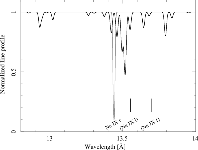
Figure 11.— Absorption line series of Fe xix between 12.8 Å and 14 Å. The Ne ix r line which blends with the complex at 13.4–13.6 Å is also shown, and the expected positions of the Ne ix i and f emission lines are indicated.

Table 7Parameters of the Absorption Line Series for Fe L-Shell Ions

Ion	$v$	$N(\mathrm{ion})$	$\xi_{0}$
	$(\rm km\,s^{-1})$	$(10^{16}\,\mathrm{cm}^{-2})$	$(\rm km\,s^{-1})$
Fe xxiv	$21^{+31}_{-30}$	$4.9^{+0.7}_{-1.0}$	$82^{+21}_{-22}$
Fe xxiii	$120^{+68}_{-94}$	$2.2^{+0.4}_{-0.2}$	$410^{+68}_{-140}$
Fe xxii	$-27^{+33}_{-35}$	$2.3^{+0.2}_{-0.4}$	$193^{+61}_{-64}$
Fe xxi	$-156^{+30}_{-29}$	$2.5^{+0.2}_{-0.4}$	$260^{+59}_{-68}$
Fe xx	$-283^{+33}_{-48}$	$3.0^{+0.3}_{-0.2}$	$333^{+57}_{-92}$
Fe xix	$-116^{+46}_{-41}$	$3.1^{+0.2}_{-0.3}$	$251^{+80}_{-68}$
Fe xviii	$-60^{+51}_{-54}$	$1.8^{+0.3}_{-0.2}$	$203^{+72}_{-56}$
Fe xvii	$-277^{+56}_{-42}$	$1.4\pm 0.3$	$78^{+26}_{-25}$

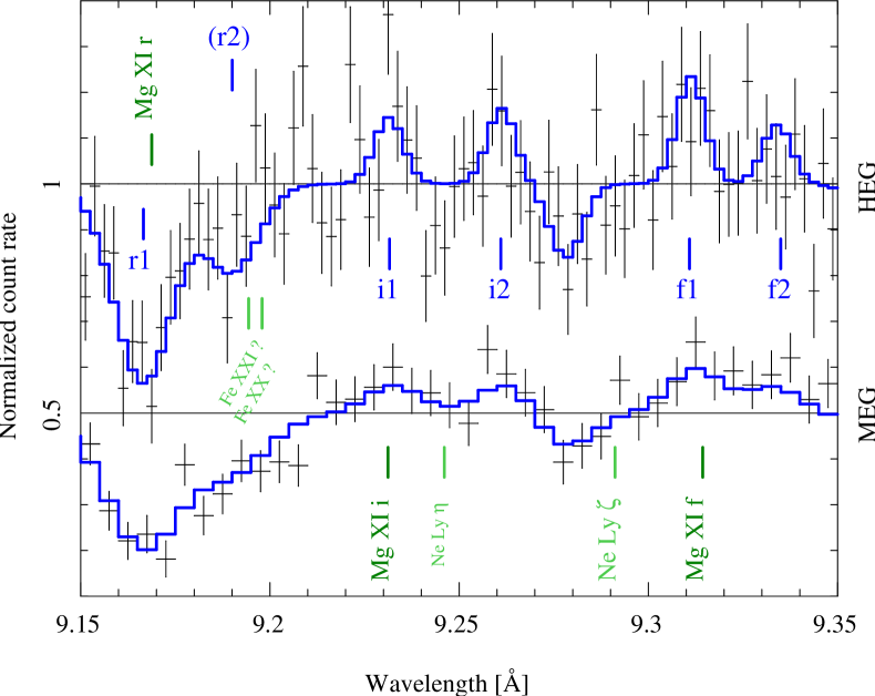
Figure 12.— Mg xi triplet of resonance (r), intercombination (i), and forbidden (f) lines in the Chandra-HETGS spectrum. The MEG data are shown with an offset of $-0.5$. While the ion/line labels indicate the rest wavelengths, the abbreviations r$n$, i$n$, and f$n$ label the actual line positions (see Table 8).

Table 8Parameters of the Lines of the Mg xi Triplet

Line	Component	$\lambda$	$v$	$W_{\lambda}$
		(Å)	(km s-1)	(mÅ)
Mg xi r	r1	$9.167^{+0.001}_{-0.002}$	$-70^{+35}_{-49}$	$-8.6^{+0.8}_{-0.7}$
Mg xi r?	(r2)	$9.190^{+0.004}_{-0.003}$	$\left(700^{+120}_{-90}\right)$	$-3.5\pm 0.9$
Mg xi i	i1	$9.232\pm 0.003$	$14^{+107}_{-105}$	$+1.5^{+1.5}_{-0.6}$
Mg xi i	i2	$9.261^{+0.002}_{-0.003}$	$968^{+52}_{-110}$	$+1.7^{+1.1}_{-0.9}$
Mg xi f	f1	$9.311^{+0.004}_{-0.001}$	$-110^{+130}_{-34}$	$+2.5^{+0.9}_{-1.2}$
Mg xi f	f2	$9.328^{+0.009}_{-0.003}$	$454^{+293}_{-111}$	$+1.3^{+0.9}_{-1.0}$

Notes. The shift velocity $v$ and equivalent width $W_{\lambda}$ are given by Equations (8) and (9). Note that the (r2) component is likely to be caused by absorption from blueshifted transitions of Fe xxi, Fe xx, and Ne x.

3.6. Emission Lines from He-Like Ions

The transitions between the 1s² ground state and the 1s2s or 1s2p excited states of He-like ions lead to the triplet of forbidden (f), intercombination (i), and resonance (r) line, see Table 4. These lines provide a density and temperature diagnostics of an emitting plasma via the ratios $R(n_{\mathrm{e}})\>:=\>F($f$)\,/\,F$(i) and $G(T_{\mathrm{e}})\>:=\>[F($i$)+F($f$)]\,/\,F$(r) of the fluxes $F$ in the r-, i-, and f-line (see, e.g., Gabriel & Jordan 1969; Porquet & Dubau 2000). In this observation, the dipole-allowed resonance transitions are seen as absorption lines, as an absorbing plasma is detected in front of the X-ray source. For the same reason, we cannot use the Fe L-shell density diagnostics (Mauche et al. 2005) as, e.g., the Fe XXII emission lines at 11.77 Å and 11.92 Å used by Mauche et al. (2003) are both seen in absorption. But we can still use the detected He-i and -f emission lines to estimate the density via the $R$-ratio, noting the caveat that the densities are systematically overestimated in the presence of an external UV radiation field, as photoexcitation of the $\mathrm{1s2s\>\left({}^{3}S_{1}\right)\rightarrow 1s2p\>\left({}^{3}P\right)}$ transition depopulates the upper level of the f-line in favor of the i-line and leads to a lower $R$-ratio (see, e.g., Mewe & Schrijver 1978; Kahn et al. 2001; Wojdowski et al. 2008).

The i- and f-lines of the Mg xi triplet are seen as two distinct components each – one with almost no shift, which is consistent with the r-absorption line, and the other one at a redshift of 400–1000 km s^-1 (see Figure 12 and Table 8). Given these two emission components and their Doppler shifts, one could be tempted to identify the absorption feature at 9.19 Å with a second redshifted Mg xi r line, but our model for the complete absorption line series (Section 3.5) predicts that the blueshifted $\mathrm{2s\rightarrow 4p}$ transitions from the ground states of Fe xxi and Fe xx, as well as the Ne x $\mathrm{1s\rightarrow 10p}$ transition, account for most of the absorption seen at 9.19 Å. Table 9 shows the $R$-ratios obtained for the two pairs of lines as well as the corresponding densities according to the calculations of Porquet & Dubau (2000, Fig. 8e), neglecting the influence of the UV radiation of HDE 226868 on the $R$-ratio. The unshifted lines would then be caused by a plasma with an electron density $n_{\mathrm{e,1}}\approx 5\!\times\!10^{12}\,$cm^-3; the redshifted pair of lines seems to stem from another plasma component with $n_{\mathrm{e,2}}\gg n_{\mathrm{e,1}}$. A more detailed discussion of these densities is presented in Section 4.1.

Table 9Electron Densities Corresponding to $R=F(\mathrm{f})/F(\mathrm{i})$ Ratios

		Model Calculations by
		Porquet & Dubau (2000)a
		$R$(Mg xi)	$n_{\mathrm{e}}$
Component	Measurement		($10^{12}\,$cm${}^{-3})$
First pair		2.3	1.0…4.5
of i and f lines	$R_{1}($Mg xi$)=1.6^{+0.7}_{-0.6}$ $\Big{\{}$	1.6	3.5…10
(unshifted)		1.0	8 …22
Second pair		1.3	5…15
of i and f lines	$R_{2}($Mg xi$)=0.8\pm 0.5$ $\Big{\{}$	0.8	12…28
(redshifted)		0.3	43…91

Note. ^a A temperature between 0.3 and 8 MK is assumed
and UV-photoexcitation is not considered.

The S/N of the spectrum above 20 Å is not high enough to describe the O vii triplet. The Ne ix triplet blends with several Fe xix lines (Figure 11). Na x i- and f-lines are likely to be present with several components, but those cannot be distinguished clearly. Similar as for Mg, there are also two i-lines of Al xii at shifts of $-477^{+120}_{-240}$ km s^-1 and $+333^{+156}_{-228}$ km s^-1, respectively, but no f-line is detected due to a blend with the strong Mg xi He $\beta$ absorption line and especially an Fe xxii 1s²2s2p(2s$\rightarrow$5p) absorption line at 7.87 Å. Similarly, the Si xiii i-line is not detected as it overlaps with absorption features probably due to nearly neutral Si K-edge structures. (Furthermore, the flux of the Si xiii f-line might be underestimated as it blends with the Mg xii Ly $\gamma$ line.) The i- and f-lines of He-like sulfur are detected with $R($S xv$)=0.61^{+1.31}_{-0.60}$, but S xv has not been modeled by Porquet & Dubau (2000). Below 4 Å, the S/N below is again not high enough to resolve further triplets from heavier elements such as argon, calcium, or iron.

4. Discussion And Conclusions

In the following, we discuss our results and derive constraints on the stellar wind in the accretion region.

4.1. Velocity and Density of the Stellar Wind

While a spherically symmetric model for the stellar wind in the HDE 226868/Cyg X-1 system can be excluded by observations (see, e.g., Gies & Bolton 1986b; Gies et al. 2003; Miller et al. 2005; Gies et al. 2008), a symmetric velocity law

$$v(r)\;\;=\;\;v_{\infty}\;\cdot\;f(r/R_{\star})$$ (12)

is usually assumed to obtain a first estimate of the particle density in the wind. The fraction $f$ of the terminal velocity $v_{\infty}$ is often parameterized by (Lamers & Leitherer 1993, Equation 3)

$$f(x)\;\;=\;\;f_{0}\>\;+\>\;\left(1-f_{0}\right)\cdot\left(1-1/x\right)^{\beta}\quad(\mbox{for }x\geq 1)$$ (13)

with $f_{0}:=v_{0}/v_{\infty}$, where $v_{0}$ is the velocity at the base of the wind ($x=1$). The simple model for the radiatively driven wind of isolated stars by Castor et al. (1975) is obtained for $\beta=1/2$. The photoionization of the wind, however, suppresses its acceleration (Blondin 1994), such that a smaller $f$ (e.g., a larger $\beta$ within the same model) is required in the Strömgren zone. Gies & Bolton (1986b) have explained the orbital variation of the 4686 Å He ii emission line profile of Cyg X-1 with a similar model for the focused wind, where $v_{\infty}$, $R_{\star}$, and $\beta$ depend on the angle $\theta$ from the binary axis. $\beta$ was interpolated between 1.60 and 1.05 for $\theta$ between $0$ and $20^{\circ}$. The value $\beta(\theta\!=\!20^{\circ})=1.05$ is, however, often used for a spherically symmetrical wind as well (Lachowicz et al. 2006; Szostek & Zdziarski 2007; Poutanen et al. 2008). Vrtilek et al. (2008) use $f_{0}=0.01$ to avoid numerical singularities and fit the (relatively low) value $\beta\approx 0.75$ to their models for UV lines. $v_{0}$ is likely to be of the order of the thermal velocity of H atoms, which is $(2kT/m_{\mathrm{H}})^{1/2}=23\,$km s^-1 and corresponds to $f_{0}=0.011$ for HDE 226868’s effective temperature $T_{\mathrm{eff}}=32$ 000 K and $v_{\infty}=2100\,$km s^-1 (Herrero et al. 1995).

Table 10Solutions to Equation (15) for the Model of Equation (13)

$n_{\mathrm{H}}(x)$	$d(x)$	$f_{0}$	$\beta$	$x$	$2100\cdot f(x)$
(1010 cm-3)		$=v_{0}/v_{\infty}$		$=r/R_{\star}$	for $\beta=\beta_{\mathrm{max}}$
440	200	0.005	$<\infty$	1	11
110	50	0.011	$\leq 1$	$\leq 1.01$	$\leq 41$
110	50	0.011	$\leq 2$	$\leq 1.08$	$\leq 36$
110	50	0.011	$\leq 3$	$\leq 1.18$	$\leq 30$
22	10	0.011	$\leq 1$	$\leq 1.08$	$\leq 180$
22	10	0.011	$\leq 2$	$\leq 1.29$	$\leq 127$
22	10	0.011	$\leq 3$	$\leq 1.48$	$\leq\phantom{1}95$
4.4	2	0.011	$\leq 1$	$\leq 1.36$	$\leq 570$
4.4	2	0.011	$\leq 2$	$\leq 1.69$	$\leq 368$
4.4	2	0.011	$\leq 3$	$\leq 1.97$	$\leq 271$

Note. The binary separation $a=41\,R_{\odot}$ corresponds to $x_{a}=a/R_{\star}=2.4$.

With the mean molecular weight per H atom, $\mu\approx 1.4$, the continuity equation $\dot{M}_{\star}\;=\;\mu\,m_{\mathrm{H}}\,n_{\mathrm{H}}(r)\>\cdot\>4\pi r^{2}\,v(r)$ gives the following estimate for the hydrogen density profile:

$$n_{\mathrm{H}}(r)\;=\;\frac{\dot{M}_{\star}/(\mu\,m_{\mathrm{H}})}{4\pi R_{\star}^{2}v_{\infty}}\>\cdot d(r/R_{\star})\;\;\mathrm{with}\;\;d(x)\;=\;x^{-2}/f(x)$$ (14)

Using the parameters of HDE 226868 ($\dot{M}_{\star}=3\!\times\!10^{-6}\,M_{\odot}\,\mathrm{yr}^{-1}$, $R_{\star}=17\,R_{\odot}$; Herrero et al. 1995; also summarized by Nowak et al. 1999, Table 1), Equation (14) predicts

$$n_{\mathrm{H}}(r)\;\;=\;\;2.2\!\times\!10^{10}\,\mathrm{cm}^{-3}\;\cdot\;d(r/R_{\star})\;\;.$$ (15)

Equation (14) can only be solved within the model of Equation (13) – or any other model for $f$ in Equation (12) with $f(x)\geq f_{0}$ – for

$$d\;\;<\;\;f_{0}^{-1}\quad\quad\mbox{and}\quad\quad 1\;\;\leq\;\;x\;\;\leq\;\;\sqrt{1/(f_{0}d)\;}\;\;.$$ (16)

For $f_{0}\approx 0.01$, the value $d\approx 190$ – which would be required to explain the density $n_{\mathrm{H,1}}\approx 4.2\!\times\!10^{12}\,$cm^-3 obtained from the unshifted Mg xi triplet (Section 3.6) – can never be reached within our model for the continuous spherical wind. This result shows that the density is likely to be overestimated by an $R$-ratio analysis which ignores the strong UV-flux of the O9.7 star. Table 10 lists therefore some solutions to Equation (15) for much lower densities as well. Due to the additional constraint that the radial velocity is less than 100 km s^-1 (Table 8), we suggest that the first emission component stems from close to the stellar surface. Although the simple wind model of Equation (13) may not be appropriate in this region, the results of Table 10 are rather insensitive to the assumptions on the velocity law, as a wide range of $\beta$ values was considered, but mostly depend on the wind’s initial velocity $v_{0}$, for which we have used a reasonable estimate. Note that $f_{0}$ and $d$ also depend on $v_{\infty}$, but their product, which is important in Equation (16), does not.

In spite of the systematic errors of the (absolute) density analysis with the $R$-ratio, we infer that the second plasma component is much denser relative to the first one. As it is seen at a larger redshift of 400–1000 km s^-1, we favor its identification with the focused wind. The two emission components could also be caused coincidentally by dense clumps in the stellar wind (which are common for O-stars; e.g., Oskinova et al. 2007; Lépine & Moffat 2008), but the interpretation as a slow base of the wind close to the stellar surface and a focused wind between the accreting black hole and its donor star provides a consistent description of both emission components: an undisturbed wind (with $v_{\infty}$ and $f_{0}$ as above, and $\beta=1.05\rightarrow 1.6$) would reach a velocity of $v(a)\approx 900\leftarrow 1200$ km s^-1 in the distance of the black hole. The focused wind in the orbital plane would then be detected with a projected velocity $v(a)\sin i=500\leftarrow 700$ km s^-1 at $\phi_{\mathrm{orb}}=0$. While photoionization reduces the efficiency of acceleration for the spherical wind, the denser focused wind is less strongly affected due to self-shielding and reaches the expected velocity. It is an observational fact that the focused wind has another ionization structure: optical emission lines (H$\alpha$, He ii $\lambda 4686$) from ions which only exist at a low ionization parameter have been observed in the focused stream (see, e.g., Gies & Bolton 1986b; Ninkov et al. 1987b; Gies et al. 2003). For the spherical wind, however, Gies et al. (2008) have conjectured that the part between Cyg X-1 and the donor star might be completely ionized in the soft state. Our observations show that the situation in the hard state may be similar.

4.2. Modeling of the Photoionization Zone

We use the photoionization code XSTAR 2.1ln7b (Kallman & Bautista 2001) to model the photoionization zone. As the latter is quite complex (due to the inhomogeneous wind density, which is strongly entangled with the X-ray flux), we do not claim to describe the photoionized wind self-consistently, but only want to derive a first approximation. For an optically thin plasma, the relative population of a given atom’s ions is merely a function of the ionization parameters

$$\xi(r)\;\;=\;\;\frac{L}{n_{\mathrm{H}}\,r^{2}}\;\;=\;\;\frac{L_{37}}{n_{13}\,r_{12}^{2}}\;\;\mathrm{erg}\;\mathrm{cm}\;\mathrm{s}^{-1}\;\;,$$ (17)

where $L_{37}$ is the ionizing source luminosity above 13.6 eV in $10^{37}\,\mathrm{erg}\;\mathrm{s}^{-1}$, $n_{13}$ is the hydrogen density in $10^{13}\,\mathrm{cm}^{-3}$ and $r_{12}$ is the distance from the source in $10^{12}\,\mathrm{cm}$.

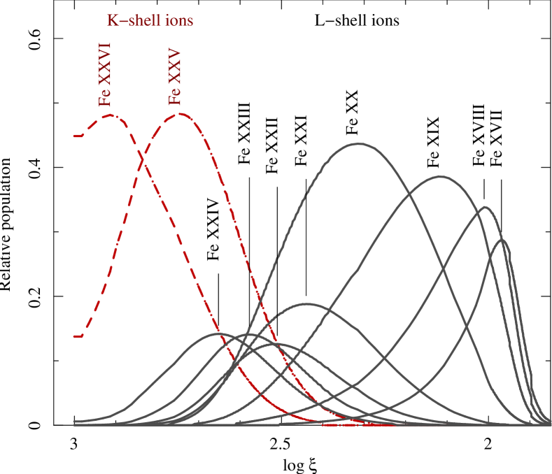
Figure 13.— Relative population of the ionization stages of iron as a function of the ionization parameter $\xi=L/(n_{\mathrm{H}}\,r^{2})$, as calculated with XSTAR for $L_{37}=3.5$ and $n_{13}=0.01$.

Table 11Ionization Parameters for Peak Ion Populations

Ion	log$\>\xi$	FWHM(log$\>\xi$)	$r_{12}=\left(L_{37}/n_{13}/10^{\log\xi}\right)^{1/2}$
Fe xxvi	2.91	0.27	0.6–0.8
Fe xxv	2.75	0.32	0.7–1.0
Fe xxiv	2.65	0.30	0.8–1.1
Fe xxiii	2.58	0.28	0.8–1.1
Fe xxii	2.51	0.31	0.9–1.3
Fe xxi	2.44	0.36	0.9–1.4
Fe xx	2.32	0.44	1.0–1.7
Fe xix	2.12	0.40	1.2–1.9
Fe xviii	2.01	0.23	1.6–2.0
Fe xvii	1.97	0.14	1.8–2.1
Ca xx	2.69	0.56	0.7–1.2
Ca xix	2.39	0.54	0.9–1.6
Ar xviii	2.55	0.65	0.7–1.5
Ar xvii	2.22	0.50	1.0–1.8
S xvi	2.38	0.69	0.8–1.7
S xv	2.08	0.43	1.2–2.0
Si xiv	2.21	0.65	0.9–2.0
Si xiii	1.96	0.39	1.5–2.4
Si iv	1.09	0.18	4.7–5.7
Mg xii	2.06	0.58	1.2–2.3
Mg xi	1.82	0.31	1.8–2.6
Ne x	1.94	0.40	1.6–2.5
Ne ix	1.74	0.24	2.1–2.8
O viii	1.80	0.26	1.9–2.6
O vii	1.62	0.22	2.5–3.2
N v	1.51	0.01	3.25–3.30
C iv	1.48	0.19	3.3–4.1

Notes. We list the range in ionization parameter and distance for the maximum ion population (Figure 13) obtained in an XSTAR simulation with $L_{37}=3.5$ and $n_{13}=0.01$. Note that the binary separation in units of $10^{12}\,$cm is $a_{12}=2.9$.

For Cyg X-1 as observed in the hard state, extrapolation of the unabsorbed model obtained by our analysis (Table 2) gives $L_{37}\approx 3.5$. Although there are obviously strong variations in the density, the XSTAR calculation has been performed with constant $n_{13}=0.01$, which is the average of $n_{\mathrm{H}}(r)$ from Equation (15) for $R_{\star}\leq r\leq a$. Figure 13 shows the resulting population of Fe ions. The ionization parameters at which the population distributions of some ions of interest peak, as well as the corresponding full width at half maximum (FWHM), are presented in Table 11. We have also included Si iv, N v, and C iv for a comparison with the work of Vrtilek et al. (2008) and Gies et al. (2008). The H- and He-like ions detected with Chandra only appear at considerable distance from the X-ray source. Taking into account that the photons emanating from Cyg X-1 first propagate through a lower density wind and that the (eventually stalled) wind of higher density is only reached in the vicinity of the star, the actual distances will be even larger than the $r_{12}$ values quoted in Table 11.

4.3. Origin of Redshifted X-Ray Absorption Lines

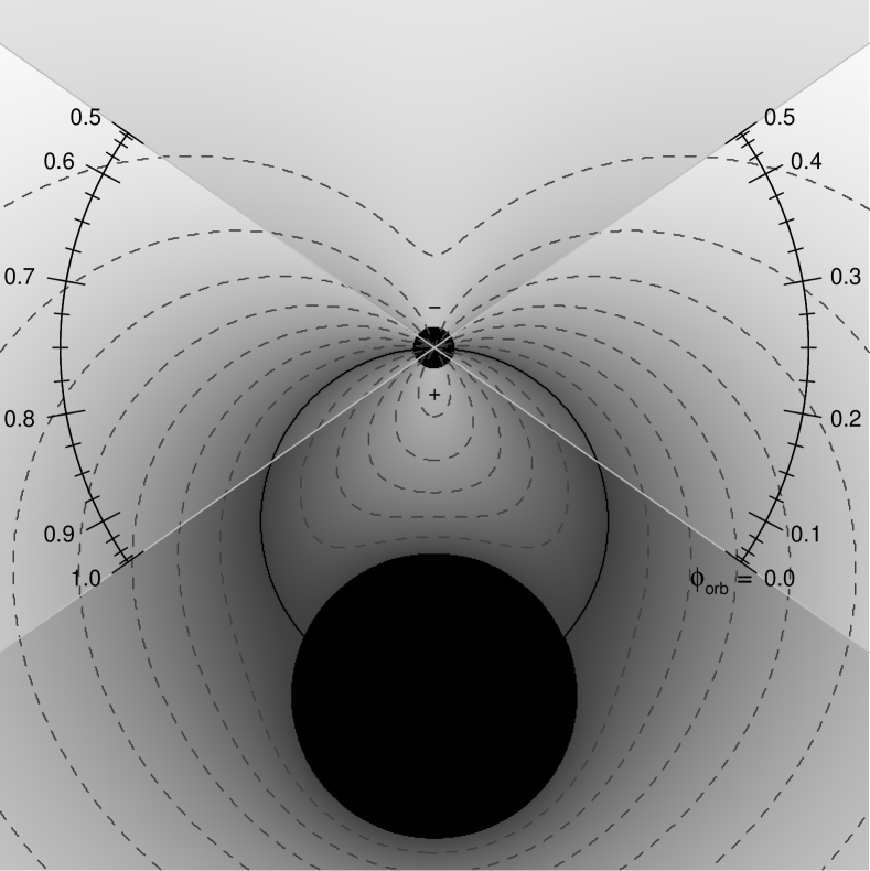
Figure 14.— Gray-scale image of $v_{\mathrm{rad,BH}}(\boldsymbol{r})$ of Equation (18), i.e., projected wind velocity against the black hole. A spherically symmetric velocity law given by Equations (12) and (13) with $v_{\infty}=2100\,\mathrm{km\,s}^{-1}$, $f_{0}=0.01$, and $\beta=1.05$ is assumed. The star and the black hole are shown as filled black circles; the size of the latter is the accretion radius $2GM_{\mathrm{BH}}/v(a)^{2}$. On the black circle passing through the center of the star and through the black hole $v_{\mathrm{rad,BH}}(\boldsymbol{r})$ is $0$ since $\alpha(\boldsymbol{r})=90^{\circ}$. Positive velocities (+) are seen only within this circle; a lighter gray means a larger redshift. Negative velocities ($-$) can likewise only occur outside of this circle; a lighter gray here means a larger blueshift. The dashed gray lines of constant $v_{\mathrm{rad,BH}}$ are shown from $-1400\,$km s^-1 to $+1000$ km s^-1 in steps of 200 km s^-1. The two highlighted sectors contain all observable lines of sight toward the black hole (after rotation in this plane) for the inclination $i=35^{\circ}$. The labels show the corresponding orbital phases.

Additional constraints on the accretion flow can be derived by considering the Doppler shifts observed in absorption lines (Sections 3.4 and 3.5). Models for the wind velocity like that of Equations (12) and (13) predict a velocity $\boldsymbol{v}(\boldsymbol{r})$ at the position $\boldsymbol{r}$ in the stellar wind. But only the projection of $\boldsymbol{v}$ against the black hole, $v_{\mathrm{rad,BH}}$, can eventually be observed as radial velocity in an X-ray absorption line. With the angle $\alpha(\boldsymbol{r})$ between $\boldsymbol{v}(\boldsymbol{r})$ and the direction from $\boldsymbol{r}$ toward the black hole, $v_{\mathrm{rad,BH}}(\boldsymbol{r})$ is

$$v_{\mathrm{rad,BH}}(\boldsymbol{r})\;\;=\;\;\cos\alpha(\boldsymbol{r})\;\cdot\;|\boldsymbol{v}(\boldsymbol{r})|\;\;.$$ (18)

Assuming a velocity field with radial symmetry with respect to the star, $\alpha(\boldsymbol{r})$ is just the angle at $\boldsymbol{r}$ between the star and the black hole. For example, $\alpha$ is $90^{\circ}$ (and $v_{\mathrm{rad,BH}}$ is therefore 0) on the sphere containing the center of the star and the black hole diametrically opposed. Redshifted absorption lines can only be observed from wind material inside this sphere, while the part of the wind outside of it is always seen at a blueshift – a fact which is independent of the assumed velocity field as long as it is directed radially away from the star.

For a spherically symmetrical wind model, any line of sight can be rotated to an equivalent one in a half-plane limited by the binary axis. Only a sector with half-opening angle $i$ can be observed unless the system’s inclination is $i=90^{\circ}$. Figure 14 shows the projected velocity $v_{\mathrm{rad,BH}}(\boldsymbol{r})$ for a simple wind model and two sectors containing all observable lines of sight toward Cyg X-1 for an inclination of $i=35^{\circ}$.

We now investigate the region where the projected wind velocity (Figure 14) is compatible with the observed Doppler shifts (Tables 5 and 7). We are confident that this method allows for the identification of the absorption regions, as the low observed velocities are always found close to the $\alpha=90^{\circ}$ sphere – independent of the wind model. For most of the investigated ions (Ne x, Mg xii, Si xiv and xiii, S xv, Ar xvii, Fe xix and xviii) the inferred distance from the black hole agrees with the predictions of Table 11, e.g., the projected velocity $-117\,$km s${}^{-1}\leq v_{\mathrm{Ne\,X}}\leq-69\,$km s^-1 measured for Ne x is (during $0.93\leq\phi_{\mathrm{orb}}\leq 1$) obtained at $r_{12}=1.78\pm 0.07$. For many other ions, both results are still very similar: e.g., Ne ix with $-214\,$km s${}^{-1}\leq v_{\mathrm{Ne\,IX}}\leq-123\,$km s^-1 is expected at $r_{12}=1.95\pm 0.07$ from the $v_{\mathrm{rad,BH}}$ model and at $r_{12}=2.1$–2.8 from the photoionization model. Only for the highly ionized iron lines, the small distances are – as already anticipated in Section 4.2 – underestimated by the XSTAR simulation run with constant average density, which overestimates the wind density close to the black hole. For example, the velocity range $-9\,$km s${}^{-1}\leq v_{\mathrm{Fe\,XXIV}}\leq 52\,$km s^-1 measured for Fe xxiv corresponds to $r_{12}=1.51\pm 0.07$, while the population of this ion peaks at $r_{12}=0.8$–1.1 within the model presented in Table 11.

4.4. Previous Chandra Observations

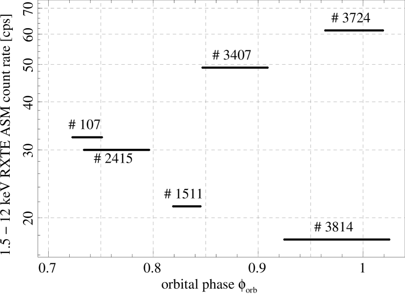
Figure 15.— Orbital phase and mean ASM count rate of the previously reported Chandra observations of Cyg X-1 (ObsID 3814 is presented in this paper).

In previous Chandra-HETGS observations of Cyg X-1, the stellar wind was seen under different viewing angles, or the X-ray source was in other spectral states (see Figure 15), which probably means that the properties of the wind were also different. Schulz et al. (2002) have analyzed the 14 ks observation ObsID 107 performed in 1999 October (at $\phi_{\mathrm{orb}}\approx 0.74$), when Cyg X-1 was in a transitional state. They derive a neutral column density of $N_{\mathrm{H}}=6.2\!\times\!10^{21}\>\mathrm{cm}^{-2}$ from prominent absorption edges (see also Table 3) and detect some emission and absorption lines with indications of P Cygni profiles. Miller et al. (2005) have investigated the focused wind with the 32 ks observation ObsID 2415 of Cyg X-1 in an intermediate state, performed in 2001 January (at $\phi_{\mathrm{orb}}\approx 0.77$). They report absorption and emission lines of H- and He-like resonance lines of Ne, Na, Mg, and Si with a mean redshift of $\approx$100 km s^-1, as well as some lines of highly ionized Fe and Ni. The column density is $6.2\!\times\!10^{21}\>\mathrm{cm}^{-2}$ (Miller et al. 2002). Marshall et al. (2001) describe Ly $\alpha$ and He $\alpha$ absorption lines, redshifted by $(450\pm 150)\>\mathrm{km\,s}^{-1}$ from the 12.6 ks observation ObsID 1511 of Cyg X-1 in the hard state, performed in 2001 January (at $\phi_{\mathrm{orb}}\approx 0.83$). Chang & Cui (2007) report dramatic variability in the 30 ks observation ObsID 3407 performed in 2001 October (at $\phi_{\mathrm{orb}}\approx 0.88$), when Cyg X-1 reached its soft state. While a large number of absorption lines (mostly redshifted, but not by a consistent velocity) is identified in the first part of their observation, most of them weaken significantly or cannot be detected at all during the second part. The complete ionization of the wind due to a sudden density decrement is given as a possible explanation. Feng et al. (2003) detect asymmetric absorption lines with the 26 ks observation ObsID 3724 of Cyg X-1 in the soft state, performed in 2002 July (at $\phi_{\mathrm{orb}}=0$). The line centers are almost at their rest wavelengths, but the red wings are more extended, especially for the transitions of highest ionized ions, which they explain by the inflowing focused wind reaching both the highest redshift and ionization parameter closest to the black hole.

The interpretation of the absorption lines presented in the previous section describes our observation consistent with wind and photoionization models. It can, however, not be applied to all of the other observations; the model of Figure 14 neither predicts a conspicuously high redshift at $\phi_{\mathrm{orb}}\approx 0.83$ and at a higher soft X-ray flux (ObsID 1511), nor a positive redshift at $\phi_{\mathrm{orb}}\approx 0.77$ at a still higher flux (ObsID 2415, see Figure 15). Inhomogeneities (e.g., density enhancements in shielding clumps) and asymmetries of the wind (e.g., due to noninertial forces in the binary system) may therefore play an important role in these cases.

4.5. Summary

In this paper, we have presented a Chandra-HETGS observation of Cyg X-1 during superior conjunction of the black hole, which allows us to detect the X-ray absorption signatures of the stellar wind of HDE 226868. The light curve near $\phi_{\mathrm{orb}}=0$ is shaped by absorption dips; these are, however, excluded from this analysis by selecting nondip times of high count rate only. At a flux of $\sim$0.25 Crab, we have to deal with moderate pile-up in the grating spectra, for which can be accounted very well with the simple_gpile2 model. The continuum of both Chandra’s soft and RXTE’s broadband X-ray spectrum has been described consistently by a single model, consisting of an empirical broken power-law spectrum with high-energy cutoff (which is typical for the hard state) and a subordinated disk component with an inner radius close to the ISCO. The joint modeling of both spectra reveals the presence of both a narrow and a relativistically broadened fluorescence Fe K$\alpha$ line. Chandra has resolved absorption edges of neutral atoms with an overabundance of metals, suggesting an origin not only in the ISM, but also in the stellar wind of the evolved supergiant. The previously suspected anticorrelation of neutral column densities and X-ray flux, which is due to photoionization, is confirmed. Absorption lines of highly ionized ions are produced where the wind becomes extremely photoionized. For H- and He-like ions, Lyman and He-series are detected up to the Ly or He$\>\epsilon$ line, which we use to measure the column density and velocity of absorbing ions. For the wealth of Fe L-shell transitions, column densities can best be obtained by directly using a physical model for the complete line series of an ion. The nondip spectrum shows almost no Doppler shifts, probably indicating that we have excluded the focused wind by our selection of nondip times. We have also detected two plasma components in emission by two pairs of i- and f-lines of He-like Mg xi. The first one is roughly at rest and we identify it with the base of the spherical wind close to the stellar surface. The second plasma component is denser and observed at a redshift that is compatible with the focused wind. A simple XSTAR simulation indicates that most of the observed ions only exist in a distance of the black hole, where the velocity of a spherical wind, projected against the black hole, is low – which is a consistent explanation of the small Doppler shifts observed in absorption lines. We review the previously reported Chandra observations of Cyg X-1 and find that not all of them can be described in the same picture, as the wind may be affected by asymmetries or inhomogeneities. A detailed spectroscopy of the absorption dips, which might shed more light on the focused wind, will be presented in a subsequent paper.

References

- Bałucińska-Church et al. (1995) Bałucińska-Church, M., Belloni, T., Church, M.J., & Hasinger, G. 1995, A&A, 302, L5
- Bałucińska-Church et al. (2000) Bałucińska-Church, et al. 2000, MNRAS, 311, 861
- Belloni et al. (1996) Belloni, T., et al. 1996, ApJ, 472, L107
- Blondin (1994) Blondin, J.M. 1994, ApJ, 435, 756
- Bolton (1972) Bolton, C.T. 1972, Nature, 240, 124
- Bondi & Hoyle (1944) Bondi, H., & Hoyle, F. 1944 MNRAS, 104, 273
- Bowyer et al. (1965) Bowyer, S., Byram, E.T., Chubb, T.A., & Friedman, H. 1965, Science, 147, 394
- Brocksopp et al. (1999) Brocksopp, et al. 1999, MNRAS, 309, 1063
- Cadolle Bel et al. (2006) Cadolle Bel, M., et al. 2006, A&A, 446, 591
- Canizares et al. (2005) Canizares, C.R., et al. 2005, PASP, 117, 1144
- Castor et al. (1975) Castor, J.I., Abbott, D.C., & Klein, R.I. 1975, ApJ, 195, 157
- Chang & Cui (2007) Chang, C., & Cui, W. 2007 ApJ, 663, 1207
- Conti (1978) Conti, P.S. 1978 A&A, 63, 225
- CXC (2005) Chandra X-ray Center 2005, The Chandra ABC Guide to Pileup, http://cxc.harvard.edu/ciao/download/doc/pileup_abc.ps
- CXC (2006) Chandra X-ray Center 2006, The Chandra Proposers’ Observatory Guide, http://cxc.harvard.edu/proposer/POG/
- Davis (2002) Davis, J.E. 2002, in High Resolution X-ray Spectroscopy with XMM-Newton and Chandra, ed. G. Branduardi-Raymont, http://adsabs.harvard.edu/abs/2002hrxs.confE..11D
- Davis (2003) Davis, J.E. 2003, in Proc. SPIE 4851, X-Ray and Gamma-Ray Telescopes and Instruments for Astronomy, ed. J.E. Trümper, & H.D. Tananbaum (Bellingham, WA:SPIE), 101
- Dotani et al. (1997) Dotani, T., et al. 1997 ApJ, 485, L87
- Doty (1994) Doty, J.P. 1994, The All Sky Monitor for the X-ray Timing Explorer, Technical report, MIT, http://xte.mit.edu/XTE.html
- Feng et al. (2003) Feng, Y.X., Tennant, A.F., & Zhang, S.N. 2003 ApJ, 597, 1017
- Friend & Castor (1982) Friend, D.B., & Castor, J.I. 1982 ApJ, 261, 293
- Gabriel & Jordan (1969) Gabriel, A.H., & Jordan, C. 1969, MNRAS, 145, 241
- Garmire et al. (2003) Garmire, G.P., et al. 2003, in Proc. SPIE 4851, X-Ray and Gamma-Ray Telescopes and Instruments for Astronomy, ed. J.E. Truemper, & H.D. Tananbaum (Bellingham, WA:SPIE), 28
- Gies & Bolton (1982) Gies, D.R., & Bolton, C.T. 1982 ApJ, 260, 240
- Gies & Bolton (1986a) Gies, D.R., & Bolton, C.T. 1986a, ApJ, 304, 371
- Gies & Bolton (1986b) Gies, D.R., & Bolton, C.T. 1986b, ApJ, 304, 389
- Gies et al. (2003) Gies, D.R., et al. 2003, ApJ, 583, 424
- Gies et al. (2008) Gies, D.R., et al. 2008, ApJ, 678, 1237
- Gleissner et al. (2004a) Gleissner, T., et al. 2004a, A&A, 425, 1061
- Gleissner et al. (2004b) Gleissner, T., et al. 2004b, A&A 414, 1091
- Gorczyca (2000) Gorczyca, T.W. 2000, Phys. Rev. A, 61, 024702
- Gorczyca & McLaughlin (2000) Gorczyca, T.W., & McLaughlin, B.M. 2000, J. Phys. B Atom. Mol. Phys., 33, L859
- Gruber et al. (1996) Gruber, D.E., et al. 1996, A&AS, 120, C641
- Hatchett & McCray (1977) Hatchett, S., & McCray, R. 1977, ApJ, 211, 552
- Herrero et al. (1995) Herrero, A., et al. 1995, A&A, 297, 556
- Houck (2002) Houck, J.C. 2002, in High Resolution X-ray Spectroscopy with XMM-Newton and Chandra, ed. G. Branduardi-Raymont, http://adsabs.harvard.edu/abs/2002hrxs.confE..17H.
- Humphreys (1978) Humphreys, R.M. 1978, ApJS, 38, 309
- Ishibashi (2006) Ishibashi, K. 2006, Specification for finding zeroth order positions in grating data analysis, http://space.mit.edu/CXC/docs/memo_fzero_1.3.ps
- Jahoda et al. (1996) Jahoda, K., et al. 1996, in Proc. SPIE 2808, EUV, X-Ray, and Gamma-Ray Instrumentation for Astronomy, Vol. VII ed. O.H. Siegmund, & M.A. Gummin (Bellingham, WA:SPIE), 59
- Juett et al. (2004) Juett, A.M., Schulz, N.S., & Chakrabarty, D. 2004, ApJ, 612, 308
- Juett et al. (2006a) Juett, A.M., Schulz, N.S., Chakrabarty, D., & Gorczyca, T.W. 2006a, ApJ, 648, 1066
- Juett et al. (2006b) Juett, A.M., Wilms, J., Schulz, N.S., & Nowak, M.A. 2006b, BAAS, 38, 921
- Kahn et al. (2001) Kahn, S.M., et al. 2001, A&A, 365, L312
- Kalberla et al. (2005) Kalberla, P.M.W., et al. 2005, A&A, 440, 775
- Kallman & Bautista (2001) Kallman, T., & Bautista, M. 2001, ApJS, 133, 221
- Karitskaya et al. (2006) Karitskaya, E.A., et al. 2006, Inf. Bull. Variable Stars, 5678, 1
- Kirsch et al. (2005) Kirsch, M.G., et al. 2005, in Proc. SPIE 5898 UV, X-Ray, and Gamma-Ray Space Instrumentation for Astronomy, Vol. XIV, ed. O.H.W. Siegmund (Bellingham, WA:SPIE), 22
- Kortright & Kim (2000) Kortright, J.B., & Kim, S.-K. 2000, Phys. Rev. B, 62, 12216
- Kotani et al. (2000) Kotani, T., et al. 2000, ApJ, 539, 413
- Lachowicz et al. (2006) Lachowicz, P., et al. 2006, MNRAS, 368, 1025
- Lamers & Leitherer (1993) Lamers, H.J.G.L.M., & Leitherer, C. 1993, ApJ, 412, 771
- Lee et al. (2001) Lee, J.C., et al. 2001, ApJ, 554, L13
- Lee et al. (2002) Lee, J.C., et al. 2002, ApJ, 567, 1102
- Lépine & Moffat (2008) Lépine, S., & Moffat, A.F.J. 2008, AJ, 136, 548
- Levine et al. (1996) Levine, A.M., et al. 1996, ApJ, 469, L33
- Makishima et al. (2008) Makishima, K., et al. 2008, PASJ, 60, 585
- Marshall et al. (2001) Marshall, H.L., Schulz, N.S., Fang, T., Cui, W., Canizares, C.R., Miller, J.M., & Lewin, W.H.G. 2001, in X-ray Emission from Accretion onto Black Holes, ed. T. Yaqoob, & J.H. Krolik (Baltimore: John Hopkins Univ.), 45
- Mauche et al. (2003) Mauche, C.W., Liedahl, D.A., & Fournier, K.B. 2003, ApJ, 588, L101
- Mauche et al. (2005) Mauche, C.W., Liedahl, D.A., & Fournier, K.B. 2005, in AIP Conf. Ser. 774, X-ray Diagnostics of Astrophysical Plasmas: Theory, Experiment, and Observation, ed. R. Smith (New York: AIP), 133
- McConnell et al. (2002) McConnell, M.L., et al. 2002, ApJ, 572, 984
- Merloni et al. (2000) Merloni, A., Fabian, A.C., & Ross, R.R. 2000, MNRAS, 313, 193
- Mewe & Schrijver (1978) Mewe, R., & Schrijver, J. 1978, A&A, 65, 99
- Mihalas (1978) Mihalas, D. 1978, Stellar atmospheres (San Francisco, CA: W.H. Freeman)
- Miller et al. (2002) Miller, J.M., et al. 2002, ApJ, 578, 348
- Miller et al. (2005) Miller, J.M., et al. 2005, ApJ, 620, 398
- Murdin & Webster (1971) Murdin, P., & Webster, B.L. 1971, Nature, 233, 110
- Ninkov et al. (1987a) Ninkov, Z., Walker, G.A.H., & Yang, S. 1987a, ApJ, 321, 425
- Ninkov et al. (1987b) Ninkov, Z., Walker, G.A.H., & Yang, S. 1987b ApJ, 321, 438
- Nowak et al. (1999) Nowak, M.A., et al. 1999, ApJ, 510, 874
- Nowak et al. (2008) Nowak, M.A., et al. 2008, ApJ, in press (arXiv: 0809.3005)
- Oskinova et al. (2007) Oskinova, L.M., Hamann, W.-R., & Feldmeier, A. 2007, A&A, 476, 1331
- Porquet & Dubau (2000) Porquet, D., & Dubau, J. 2000, A&AS, 143, 495
- Pottschmidt et al. (2000) Pottschmidt, K., el al. 2000, A&A, 357, L17
- Pottschmidt et al. (2003) Pottschmidt, K., et al. 2003, A&A, 407, 1039
- Poutanen et al. (2008) Poutanen, J., Zdziarski, A.A., & Ibragimov, A. 2008, MNRAS, 389, 1427
- Remillard & McClintock (2006) Remillard, R.A., & McClintock, J.E. 2006, ARA&A, 44, 49
- Russell et al. (2007) Russell, D.M., Fender, R.P., Gallo, E., & Kaiser, C.R. 2007, MNRAS, 376, 1341
- Schulz et al. (2002) Schulz, N.S., et al. 2002, ApJ, 565, 1141
- Shaposhnikov & Titarchuk (2007) Shaposhnikov, N., & Titarchuk, L. 2007, ApJ, 663, 445
- Shimura & Takahara (1995) Shimura, T., & Takahara, F. 1995, ApJ, 445, 780
- Spitzer (1978) Spitzer, L. 1978, Physical processes in the interstellar medium (New York: Wiley-Interscience)
- Strömgren (1939) Strömgren, B. 1939, ApJ, 89, 526
- Szostek & Zdziarski (2007) Szostek, A., & Zdziarski, A.A. 2007, MNRAS, 375, 793
- Treves et al. (1980) Treves, A., et al. 1980, ApJ, 242, 1114
- van Aken & Liebscher (2002) van Aken, P.A., & Liebscher, B. 2002, Phys. Chem. Miner., 29, 188
- Verner et al. (1996) Verner, D.A., Verner, E.M., & Ferland, G.J. 1996, At. Data Nucl. Data Tables, 64, 1
- Verner & Yakovlev (1995) Verner, D.A., & Yakovlev, D.G. 1995, A&AS, 109, 125
- Verner et al. (1993) Verner, D.A., Yakovlev, D.G., Band, I.M., & Trzhaskovskaya, M.B. 1993, At. Data Nucl. Data Tables, 55, 233
- Vrtilek et al. (2008) Vrtilek, S.D., et al. 2008, ApJ, 678, 1248
- Walborn (1973) Walborn, N.R. 1973, ApJ, 179, L123
- Webster & Murdin (1972) Webster, B.L., & Murdin, P. 1972, Nature, 235, 37
- Wilms et al. (2000) Wilms, J., Allen, A., & McCray, R. 2000, ApJ, 542, 914
- Wilms et al. (2006) Wilms, J., et al. 2006, A&A, 447, 245
- Wojdowski et al. (2008) Wojdowski, P.S., Liedahl, D.A., & Kallman, T.R. 2008, ApJ, 673, 1023
- Xiang et al. (2005) Xiang, J., Zhang, S.N., & Yao, Y. 2005, ApJ, 628, 769
- Zhang et al. (1997) Zhang, S.N., et al. 1997, ApJ, 477, L95
- Ziółkowski (2005) Ziółkowski, J. 2005, MNRAS, 358, 851