Thermal fluctuations and phase diagrams of the phase field crystal model with pinning

Abstract

We study the influence of thermal fluctuations in the phase diagram of a recently introduced two-dimensional phase field crystal model with an external pinning potential. The model provides a continuum description of pinned lattice systems allowing for both elastic deformations and topological defects. We introduce a non-conserved version of the model and determine the ground-state phase diagram as a function of lattice mismatch and strength of the pinning potential. Monte Carlo simulations are used to determine the phase diagram as a function of temperature near commensurate phases. The results show a rich phase diagram with commensurate, incommensurate and liquid-like phases with a topology strongly dependent on the type of ordered structure. A finite-size scaling analysis of the melting transition for the $c(2\times 2)$ commensurate phase shows that the thermal correlation length exponent $\nu$ and specific heat behavior are consistent with the Ising universality class as expected from analytical arguments.

I Introduction

Many two-dimensional (2D) lattice systems on periodic potentials form different ordered structures at low temperatures which may be unstable against thermal fluctuations and the mismatch between the competing periodicities. Adsorbed layers on crystal surfaces patry ; persson ; patry07 , vortex lattices in 2D superconductors martin97 and colloidal crystals lin00 ; ling08 in a periodic substrate are important examples of current interest. In numerical simulations, pure elastic models or particle models are often employed. However, there are important limitations in these approaches. In the former, plastic deformations such as dislocations are not taken into account and in the latter, the accessible time and spatial scales may be very limited. These limitations are particularly important in atomistic simulations of crystalline materials described by microscopic models with complicated interactions, where the time scale is set by the vibrational frequency and consequently relatively small system sizes are often used in numerical simulations.

Recently, a phase field crystal (PFC) model for pinned lattice systems was introduced achim06 that allows for both elastic and plastic deformations of the lattice. The model describes the lattice system as a continuous density field in an external pinning potential. In this formulation a free energy functional is introduced which depends on the phase field $\psi(\vec{r})$ corresponding to the particle density. In absence of a pinning potential, the free energy is minimized when $\psi$ is spatially periodic elder02 forming a hexagonal solid phase in 2D. By incorporating phenomena on short length scales the model naturally includes elastic and plastic deformations and it should be computationally more efficient than particle simulations such as standard molecular dynamics elder02 ; elder04 .

In a previous work achim06 , the phase diagram of the PFC model in a periodic pinning potential with square symmetry was determined as a function of the pinning strength and lattice mismatch, in the absence of thermal fluctuations. A numerical minimization procedure was used to determine the different ordered phases and the phase transitions, based on the corresponding dynamical equation of motion for a conserved field. In the present work, we consider the influence of thermal fluctuations and lattice mismatch in the PFC model with pinning. We first introduce a non-conserved version of the model which is more efficient for equilibrium simulations, such that a constant chemical potential is included in the free energy to fix the average density. With this new version, we determine the ground-state phase diagram as a function of lattice mismatch and strength of pinning potential using the corresponding non-conserved dynamical equations of motion. Monte Carlo (MC) simulations are then used to determine the phase diagram as a function of temperature and mismatch near commensurate phases. The results reveal that the model has a rich phase diagram, which includes commensurate, incommensurate and liquid-like phases with a topology dependent on the type of ordered structure. In particular, a finite-size scaling analysis of the melting transition for the $c(2\times 2)$ commensurate phase shows that the thermal correlation length exponent $\nu$ and specific heat behavior are consistent with the Ising universality class, which is expected from analytical arguments based on symmetry considerations and Landau free-energy expansion.

II Model

The mean field free-energy functional of the PFC model with an external pinning potential achim06 can be written in dimensionless units as

$$F=F_{0}\int d\vec{x}\{\frac{1}{2}\psi[r+(1+\nabla^{2})^{2}]\psi+\frac{\psi^{4}}{4}+V\psi\},$$ (1)

where $\psi(\vec{x})$ is a continuous field representing the local number density of the particles and $V(\vec{x})$ represents the external pinning potential. The overall constant $F_{0}$ sets the energy scale and $r$ is a parameter. In Eq. (1), $\psi(\vec{x})$ is a conserved field and the minima of the free energy depends on the average value of $\psi(\vec{x})$. To remove this conservation constraint on $\psi(\vec{x})$, we introduce here an additional linear term to the free energy containing the chemical potential $\mu$, which controls the average value of $\psi(\vec{x})$. This leads to a model mean field free-energy functional

$$F=F_{0}\int d\vec{x}\{\frac{1}{2}\psi[r+(1+\nabla^{2})^{2}]\psi+\frac{\psi^{4}}{4}+V\psi-\mu\psi\}.$$ (2)

This modification allows the use of a MC algorithm with non-conserved dynamics as described in Sec. 3, which is more efficient for equilibrium simulations.

In the absence of the pinning potential, $V(\vec{x})=0$, the free energy of Eq. (2) can be minimized by a configuration of the field $\psi(\vec{x})$ forming a hexagonal pattern of peaks with wavector of magnitude $k_{0}=1$, when the values of the parameters $r$ and $\mu$ are chosen appropriately. This structure of peaks can be regarded as a crystalline system and the free energy functional of Eq. (2) can then be used to describe both elastic and plastic properties of such a lattice system within a mean field description elder02 ; elder04 ; elder07 for temperatures $T$ below the mean field melting temperature $T_{m}$ by setting the parameter $r\propto T-T_{m}$. However, the free energy of Eq. (2) do not provide all the information on the system at finite temperatures and specially do not take into account strong thermal fluctuations which may lead to the melting of the hexagonal pattern.

To go beyond mean field theory and take thermal fluctuations into account, we follow the usual procedure of introducing a coarse-grained effective Hamiltonian chaikin where the energy for a particular configuration of the order parameter is given by the corresponding mean field free-energy functional. Then instead of considering just the minimum energy this procedure allows for excitations according to a statistical weight provided by the free energy functional. In the present case we take as the effective Hamiltonian $H[\psi]\equiv F[\psi]$ with the corresponding partition function

$$Z=\sum_{\{\psi(\vec{x})\}}e^{-H[\psi]/k_{B}T},$$ (3)

where $T$ is the temperature and the summation (functional integration) is taken over all configurations of $\psi(\vec{x})$. Physical quantities are defined in the usual way as thermal averages over $\psi$ configurations. The parameter $r$ contained in $H[\psi]$ is taken to be a temperature-independent constant for the region below the mean field transition temperature $T_{m}$ in the absence of the pinning potential.

We consider a pinning potential $V(x,y)$ with square symmetry

$$V(x,y)=V_{0}[\cos(k_{s}x)+\cos(k_{s}y)],$$ (4)

where $k_{s}=2\pi/a_{s}$ is the wave vector of the pinning potential, which can represent, for example, and adsorbed layer on the $(100)$ face of an fcc crystal patry ; patry07 . We define the lattice misfit between the lattice system and pinning potential as $\delta_{\rm m}=(k_{0}-k_{s})/k_{0}$, where $k_{0}=1$ is the wave vector of the hexagonal periodic patternfoot1 of $\psi(x,y)$ in the absence of the pinning potential, corresponding to a free lattice system. Thus, for $\delta_{\rm m}\gg 0$, the lattice system is under tensile strain while for $\delta_{\rm m}\ll 0$ it is under compression.

III Monte Carlo simulation

The free energy associated with the partition function of Eq. (3), which now takes into account thermal fluctuations can not be obtained directly without approximations. Therefore, to obtain the equilibration configurations and average quantities it is necessary to perform numerical simulations and for this purpose we used the MC method. Thermal averages over configurations of $\psi(x,y)$ were performed using MC simulations on a discrete version of the effective Hamiltonian $H[\psi]$. The field $\psi(x,y)$ and pinning potential $V(x,y)$ are defined on a square space grid, $x=idx$, $y=jdy$ ($i,j$ integers), with grid size $L\times L$ and grid spacing $dx=dy$ and with periodic boundary conditions. The Laplacians in Eq. (2) were approximated by a simple discretization scheme

$$\frac{\partial^{2}}{\partial x^{2}}f_{i,j}=\frac{f_{i+1,j}+f_{i-1,j}-2f_{i,j}}{(\Delta x)^{2}}.$$ (5)

The standard Metropolis algorithm was used for simulations at a given temperature. At each grid site $(i,j)$, we attempt to change $\psi_{i,j}$ by an small amount $\Delta\psi$ with probability $\min(1,e^{-\Delta H/k_{B}T})$, using the Metropolis scheme, where $\Delta H$ is the resulting change in the configurational energy. Simulations were performed using, typically, $L$ ranging from $64$ to $224$, grid spacing $dx=\pi/4$ and $(4-2)\times 10^{6}$ MC passes for equilibration and equal number of passes for thermal averages. Because of the periodic boundary conditions, the length of the system $L\ dx$ has to be a multiple of the lattice constant of the pinning potential, $2\pi/k_{s}$. This condition imposes a restriction on the values of $k_{s}$ when calculations are done for fixed $L$ and $dx$. Thus, to be able to change $k_{s}$ continuously near a commensurate phase while still keeping the same system size $L$, we choose a variable grid spacing $dx=(k_{s}^{0}/k_{s})(\pi/4)$, where $k_{s}^{0}$ is fixed such that $L\pi/4=n(2\pi/k_{s}^{0})$ ($n$ is an integer). The parameters $r$ and $\mu$ were set to $r=-1/4$ and $\mu=-0.1875$, corresponding to the hexagonal crystalline region in the original PFC model without pinning elder02 ; elder04 . The temperature $T$ is measured in units of $F_{0}k_{B}^{-1}$.

Near the phase transitions where long equilibration times are required, we use the exchange MC method (parallel tempering) nemoto ; marinari . This method is known to reduce significantly the critical slowing down near phase transitions. Recently, it has being used to study glassy incommensurate vortex lattices in 2D superconducting arrays eg08 . In this method, many replicas of the system with different temperatures $T_{i}$ in a range above and below the critical temperature are simulated simultaneously and the corresponding configurations are allowed to be exchanged with a probability distribution satisfying detailed balance. The exchange process allows the configurations of the system to explore the temperature space, being cooled down and warmed up, and the system can in principle escape more easily from metastable minima at lower temperatures. Without the replica exchange step, the method reduces to conventional MC simulations performed at different temperatures. The method was implemented by performing MC simulations as described above for each replica at different temperatures, simultaneously and independently, for a few MC passes. Then exchange of pairs of replica configurations at temperatures $T_{i}$ and $T_{j}$ and energies $E_{i}$ and $E_{j}$ is attempted with probability $\min(1,\exp(-\Delta))$, where $\Delta=(1/T_{i}-1/T_{j})(E_{j}-E_{i})$, using the Metropolis scheme. We typically used $10^{6}$ MC passes for equilibration with up to $30$ replicas and equal number of MC passes for calculations of average quantities.

IV Results and discussion

IV.1 Ground-state phase diagram

The ordered structures in the ground state were obtained by simulations of the dissipative dynamical equations for the phase field $\psi(\vec{x})$, as in the previous work achim06 . The reason for using this method instead of the MC method described in Sec. III is that, at very low temperatures, MC simulations turned out to be computationally less efficient due to the low acceptance rate for MC moves. The dissipative dynamics should evolve the system to the lower-energy state for arbitrary initial conditions. Therefore the determination of the final configurations is equivalent to finding the ground state for the effective Hamiltonian in Eq. (3), since $H[\psi]\equiv F[\psi]$. For the free-energy functional of Eq. (2) with non-conserved field the dynamical equations are

$$\frac{\delta\psi}{\delta t}=-\frac{\delta F}{\delta\psi}.$$ (6)

The ground-state phase diagram was obtained by finding the final configurations where $\delta\psi/\delta t=0$ starting from different initial configurations, for different misfits $\delta_{m}$ and amplitudes of the pinning potential $V_{0}$. Typically, we start with a hexagonal structure which is the minimum energy state in the absence of the periodic potential ($V_{0}=0$) and then increase slowly $V_{0}$ to the its final value for fixed $\delta_{\rm m}$. The calculations are then repeated for different initials conditions. The ground state is the final configuration corresponding to the lowest energy.

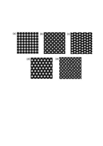
Figure 1: Density plot of the phase field $\psi(\vec{x})$ showing commensurate (C) and incommensurate (IC) structures in the ground state, depending on the amplitude of the pinning potential $V_{0}$ and misfit parameter $\delta_{\rm m}$. (a) $(1\times 1)$ C phase; (b) $c(2\times 2)$ C phase; (c) $(2\times 1)$ C phase; (d) hexagonal (full) IC phase and (e) IC phase with domain walls near the $c(2\times 2)$ C phase.

Three low-order commensurate structures were obtained as shown in Fig. 1: a $(1\times 1)$ commensurate (C) phase, where the peaks of $\psi(\vec{x})$ coincide with the pinning potential minima; a $c(2\times 2)$ C phase, where they form a superstructure with periodicity twice that of the pinning potential along the principal directions and a $c(2\times 1)$ phase where the superstructure has lattice periodicity twice the pinning potential along one of the directions. In addition, there are incommensurate (IC) phases, where $\psi(\vec{x})$ forms a hexagonal periodic structures incommensurate with the pinning potential as in Fig. 1(d) or a structure of domain walls separating commensurate regions as in Fig. 1(e).

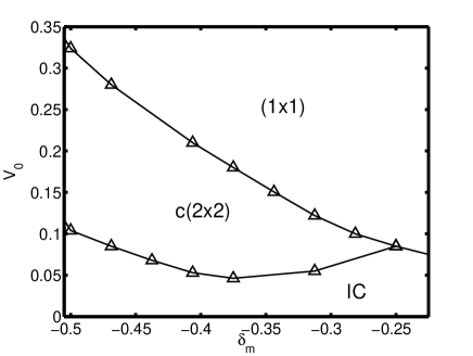
Figure 2: Ground state phase diagram in terms of the pinning strength $V_{0}$ and mismatch $\delta_{\rm m}$ for $-0.5\leq\delta_{\rm m}\leq-0.225$

The results of extensive numerical calculations using the dynamical equation (6) are summarized in the phase diagram in Fig. 2 for $-0.5\leq\delta_{\rm m}\leq-0.225$ and in Fig. 3 for $-0.2\leq\delta_{\rm m}\leq 0.40$. The transitions between the different phases were determined from the change in the structure factor.

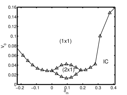
Figure 3: Ground state phase diagram in terms of the pinning strength $V_{0}$ and mismatch $\delta_{\rm m}$ for $-0.2\leq\delta_{\rm m}\leq 0.4$.

IV.2 Finite-temperature phase diagram

We have studied the influence of thermal fluctuations and lattice mismatch near the simplest commensurate structures, the $(1\times 1)$ and $c(2\times 2)$ commensurate phases, using the MC method described in Sec. III. The phase diagrams were obtained by monitoring the behavior of the structure factor and specific heat as a function of temperature and lattice misfit. First, the structure factor $S(\vec{k})$ was calculated from the positions $\vec{R}_{j}$ of the local peaks in the field $\psi(x,y)$ as

$$S(\vec{k})=\langle\sum_{j,j^{\prime}=1}^{N_{P}}\frac{1}{N_{P}}e^{-i\vec{k}\cdot(\vec{R}_{j}-\vec{R}_{j^{\prime}})}\rangle,$$ (7)

where $N_{p}$ is the number of peaks. To locate the peak positions $\vec{R}_{j}$ for each configuration of $\psi(x,y)$ we have implemented a computer algorithm ramosb to find the local maxima in $\psi(x,y)$ based on a particle location algorithm used in digital image processing crocker . Alternatively, a structure factor can also be defined directly from the field $\psi(x,y)$ as

$$S_{\psi}(\vec{k})=\frac{1}{L^{2}}\langle|\psi(\vec{k})|^{2}\rangle,$$ (8)

where $\psi(\vec{k})$ is the Fourier transform of $\psi(\vec{x})$. While the two expressions give similar results the former expression is better for characterizing a structural phase transition as it includes only the ordering of the lattice and does not simultaneously include fluctuations in the amplitude of the $\psi$ as the latter expression does. The results described here were obtained using the definition in Eq. (7). Second, the specific heat $c$ was calculated directly from the average energy as $c=(1/L^{2})(d\langle H\rangle/dT)$ and from the fluctuation relation

$$c=\frac{1}{L^{2}T^{2}}(\langle H^{2}\rangle-\langle H\rangle^{2}).$$ (9)

We checked that these two different ways of calculating $c$ gave the same results, which indicates that the system is properly equilibrated at a given temperature.

Figs. 4a and 4b show the behavior of the scaled structure-factor peak $S(k_{m})/N_{p}$ and specific heat $c$ as a function of temperature for the $(1\times 1)$ and $c(2\times 2)$ commensurate phases. Here $k_{m}$ is the magnitude of the wave-vector corresponding to the local maximum in $S(\vec{k})$. For the $(1\times 1)$ phase, $S(k_{m})/N_{p}$ in Fig. 4a decreases and broaden with temperature but does not disappear at the highest temperature where a liquid-like phase is expected. Also, there is no peak in the corresponding specific heat in Fig. 4b. This indicates that the $(1\times 1)$ phase does not melt into a liquid-like phase via a phase transition, instead there is a smooth crossover from a low temperature highly ordered phase to a high temperature phase where the pinning potential still induces some order in the peak pattern of $\psi(\vec{x})$. This behavior is expected on theoretical grounds patry ; haldane since in this case the pinning potential has the same symmetry as the commensurate phase and acts as a constant external field on the displacement order parameter. On the other hand, for the $c(2\times 2)$ commensurate phase, $S(k_{m})/N_{p}$ in Fig. 4a drops sharply near the temperature where there is a peak in the corresponding specific heat in Fig. 4b and this behavior is associated with the melting of the ordered structure into a liquid-like phase.

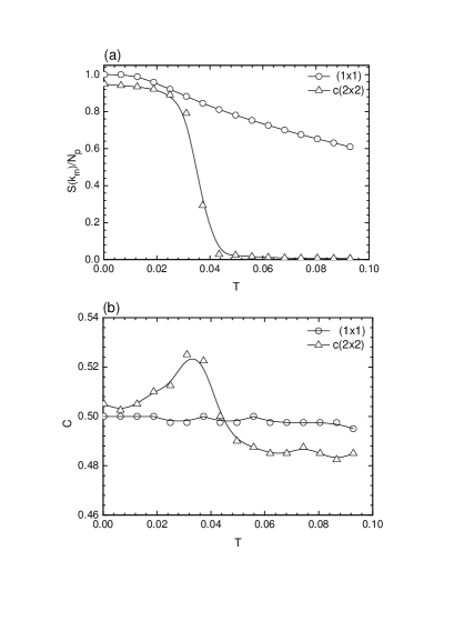
Figure 4: Temperature dependence of the scaled structure-factor peak $S(k_{m})/N_{p}$ (a) and specific heat $c$ (b) for the $(1\times 1)$ commnesurate phase ( $\delta_{\rm m}=0$, $V_{0}=0.10$ ) and $c(2\times 2)$ commensurate phase ( $\delta_{\rm m}=-0.5$, $V_{0}=0.275$). Here $k_{m}$ is the wave vector of the corresponding ordered structure.

The phase diagrams obtained near the $(1\times 1)$ and $c(2\times 2)$ commensurate phases as a function of misfit, strength of pinning potential and temperature are shown in Figs. 5 and 6, respectively. In addition to the melting transitions, there are also commensurate-incommensurate transitions from the $c(2\times 2)$ to IC phases and from $c(2\times 2)$ to $(1\times 1)$ phases which are identified by the change in the peak patterns in the structure factor. A striking feature of the phase diagram is its topology, which is strong dependent on the type of C phase. This agrees qualitatively with theoretical predictions from simplified models patry ; haldane . However, the present calculations were not sufficiently accurate to determine the joining of the transition lines near the incommensurate phases in Figs. 6(a) and (b). Hence, we were unable to investigate the theoretical predictions haldane ; rys for the existence of an intermediate liquid phase between the IC and C phases at finite temperature near the $c(2\times 2)$ commensurate phase.

Figure 5: Phase diagrams near the $(1\times 1)$ commensurate phase. (a) at fixed pinning strength $V_{0}$ and (b) at fixed misfit $\delta_{\rm m}$.

Figure 6: Phase diagrams near the $c(2\times 2)$ commensurate phase. (a) at fixed pinning strength $V_{0}$ and (b) at fixed misfit $\delta_{\rm m}$.

In addition to the topology of the phase diagram, the nature of the phase transitions between the different phases is of particular interest. We have investigated in detail the critical behavior for the simplest case, corresponding to the melting transition of the $c(2\times 2)$ commensurate phase as a function of the temperature. From symmetry considerations and Landau free-energy expansions schick , one expects that the critical behavior should be in the Ising universality class. To verify if the phase field crystal model provides a correct description of this behavior, we have performed a finite-size scaling analysis of the melting of the $c(2\times 2)$ phase as a function of temperature, for a fixed value of misfit $\delta_{\rm m}=-0.5$. Calculations were performed for increasing system sizes for the specific heat, structure factor and a suitable dimensionless Binder ratio binder . We define the Binder ratio $U_{L}(T)$ as

$$U_{L}=2-\frac{\langle|\rho(k_{m})|^{4}\rangle}{\langle|\rho(k_{m})|^{2}\rangle^{2}},$$ (10)

where the order parameter $\rho(k_{m})$ is the Fourier transform of the of density of local peaks in the field $\psi(x,y)$ at $\vec{R}_{j}$

$$\rho(k_{m})=\frac{1}{N_{P}}\sum_{j=1}^{N_{P}}e^{-i\vec{k}_{m}\cdot\vec{R}_{j}},$$ (11)

evaluated at the wave vector $k_{m}$ corresponding to the local maximum of the structure factor $S(k)$. The finite-size behavior of $U_{L}$ provides an accurate determination of the critical temperature $T_{c}$ and an estimate of the thermal critical exponent $\nu$ which characterizes the divergent correlation length, $\xi\propto|T-T_{c}|^{-\nu}$, near the transition binder ; binder97 . In the high temperature disordered phase, the real and imaginary parts of $\rho(k_{m})$ fluctuate with a Gaussian distribution leading to $U_{L}\rightarrow 0$ while at low temperature there is long-range order with $\langle\rho(k_{m})\rangle\neq 0$ and therefore $U_{L}\rightarrow 1$ for $L\rightarrow\infty$. At the critical temperature $T_{c}$, the ratio $U_{L}$ becomes independent of the system size $L$ and therefore plots of $U_{L}(T)$ as a function of temperature for different systems sizes should cross at the same point, corresponding to the critical temperature $T_{c}$ of the system in the thermodynamic limit. In the scaling regime sufficiently close to $T_{c}$, the dimensionless $U_{L}(T)$ should satisfy the scaling form

$$U_{L}(T)=\bar{U}((T-T_{c})L^{1/\nu}),$$ (12)

where $\bar{U}(x)$ is a scaling function. Since the slope ($\partial U_{L}(T)/\partial T$) evaluated at $T_{c}$ is proportional to $L^{1/\nu}$, an estimate of $\nu$ can be obtained binder97 from a log-log plot of this quantity against $L$.

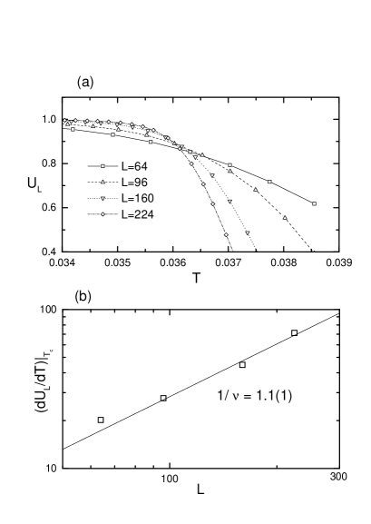
Figure 7: (a) Temperature dependence of the Binder ratio $U_{L}(T)$ for different system sizes $L$, near the melting transition of the $c(2\times 2)$ commensurate phase at $\delta_{\rm m}=-0.5$ and $V_{0}=0.275$; (b) Estimate of the thermal critical exponent $\nu$ from the log-log plot of $\frac{\partial}{\partial T}U_{L}(T)$ at $T_{c}$ against $L$ for the three largest system sizes.

Fig. 7(a) shows the temperature behavior of $U_{L}$ for different system sizes. Although the curves do not cross precisely at the same point, for the three largest system sizes the curves intersect approximately at $T_{c}\approx 0.03599(20)$. The lack of intersection at a common point should be due to statistical errors and corrections to scaling. Fig. 7b shows a log-log of $\delta U_{L}(T)/\delta T$ evaluated at the estimated $T_{c}$ against $L$ from where we obtain $1/\nu=1.1(1)$. This estimate of $\nu$ is in agreement with the exact value for the thermal exponent of the two-dimensional Ising model, $\nu=1$.

The finite-size behavior of the specific heat $c$ is also consistent with the Ising universality class, where the specific heat exponent is $\alpha=0$. Fig. 8(a) shows the temperature behavior of the specific heat for the different systems sizes. From finite-size scaling, the maximum of $c$ should scale as $L^{\alpha/\nu}$, which corresponds to a logarithmic behavior $C_{max}\propto\log L$, if $\alpha=0$. Fig. 8(b) shows that the linear-log plot of the specific heat maximum $c_{max}$ against $L$ is indeed consistent with a logarithmic behavior for the three largest system sizes.

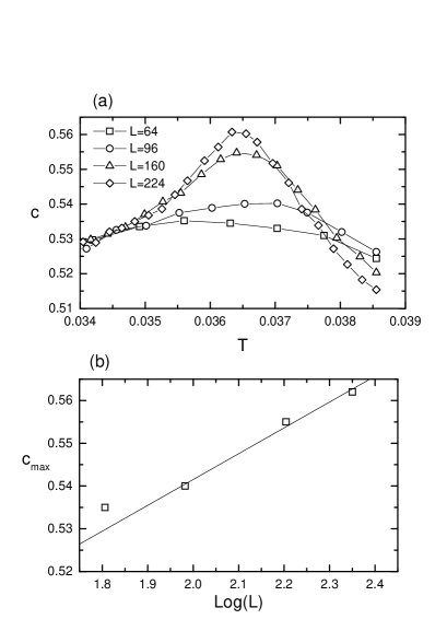
Figure 8: (a) Temperature dependence of the specific heat $c$ for different system sizes $L$, near the melting transition of the $c(2\times 2)$ commensurate phase at $\delta_{\rm m}=-0.5$ and $V_{0}=0.275$; (b) Specific heat maxima $c_{max}$ in a linear-log plot indicating a logarithmic behavior as a function of $L$ for the three largest systems sizes.

The correlation function exponent $\eta$ can also be estimated from the expected finite-size behavior of the structure factor, which should scale as $S(k_{m})\propto L^{2-\eta}$ at $T_{c}$. Fig. 9 shows a log-log plot of $S(k_{m})/L^{2}$ evaluated at the above estimated $T_{c}$ against $L$ from where we find $\eta=0.15$. Unlike the above estimates of $\nu$ and $\alpha$, this estimate of $\eta$ is much smaller than the known exact value for the Ising model, $\eta=0.25$. This large discrepancy could be due to corrections to scaling. However, to take such corrections into account would require more accurate data and larger system sizes, which is beyond the scope of the present work.

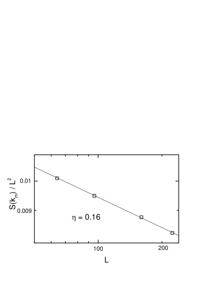
Figure 9: Estimate of the correlation function exponent $\eta$ from the log-log plot of $S(k_{m})/L^{2}$ at $T_{c}$ against $L$ for the three largest systems sizes.

V Conclusions

In the present work we have studied the effects of thermal fluctuations in the phase field crystal model with an external pinning potential achim06 using a non-conserved version of the model and Monte Carlo simulations. We have determined the phase diagram as a function of temperature and mismatch near low-order rational commensurate phases. The results show a rich phase diagram with commensurate, incommensurate and liquid-like phases with a topology dependent on the type of ordered structure qualitatively consistent with predictions of simplified models of pinned lattice systems patry ; haldane . In particular, we find that the melting transition for the $c(2\times 2)$ commensurate phase is consistent with the Ising universality class, which is expected from analytical arguments based on symmetry considerations and Landau free-energy expansion schick . Our results demonstrate that the PFC model and the MC method employed here can be used to study specific lattice systems by adjusting the parameters of the model to match the experimental structure factor elder04 ; elder07 and choosing a suitable pinning potential.

- (1) A. Patrykiejew, S. Sokolowski, and K. Binder, Surf. Sci. Rep. 37, 207 (2000).
- (2) B. Persson, Surf. Sci. Rep. 15, 1 (1992).
- (3) A. Patrykiejew and S. Sokolowski, Phys. Rev. Lett. 99, 156101 (2007).
- (4) J.I. Martin, M. Vélez, J. Nogués, and I.K. Schuller, Phys. Rev. Lett. 79, 1929 (1997).
- (5) K-H Lin, J.C. Crocker, V. Prasad, A. Schofield, D.A. Weitz, T.C. Lubensky, and A.G. Yodh, Phys. Rev. Lett. 85, 1770 (2000).
- (6) A. Pertsinidis and X.S. Ling, Phys. Rev. Lett. 100, 028303 (2008).
- (7) C.V. Achim, M. Karttunen, K.R. Elder, E. Granato, T. Ala-Nissila, and S.C. Ying, Phys. Rev. E 74, 021104 (2006); J. Phys.: Conf. Ser. 100, 072001 (2008).
- (8) K.R. Elder, M. Katakowski, M. Haataja, and M. Grant, Phys. Rev. Lett. 88, 245701 (2002).
- (9) K.R. Elder, and M. Grant, Phys. Rev. E 70, 051605 (2004).
- (10) K.R. Elder, N. Provatas, J. Berry, P. Stefanovic, and M. Grant, Phys. Rev. B 75, 064107 (2007).
- (11) P.M. Chaikin and T.C. Lubensky, Principles of condensed matter physics, Cambridge University Press, 1995.
- (12) The wave-vector of the periodic lattice is strictly only one in a one-mode approximation and may deviate by a few percent when higher order modes are considered.
- (13) K. Hukushima and K. Nemoto, J. Phys. Soc. Jpn. 65, 1604 (1996).
- (14) E. Marinari and G. Parisi, Europhys. Lett. 19, 451 (1992).
- (15) E. Granato, Phys. Rev. Lett. 101, 027004 (2008).
- (16) J.A.P. Ramos, E. Granato, C.V. Achim, M. Karttunen, S.C. Ying, K.R. Elder, and T. Ala-Nissila, unpublished.
- (17) J.C. Crocker and D. G. Grier, J. Colloid Interface Sci. 179, 298 (1996).
- (18) F.D.M. Haldane, P. Bak, and T. Bohr, Phys. Rev. B 28, 2743 (1983).
- (19) F.S. Rys, Phys. Rev. Lett. 51, 849 (1983).
- (20) M. Schick, Prog. Surf. Sci. 11, 245 (1981).
- (21) K. Binder, Phys. Rev. Lett. 47, 693 (1981).
- (22) K. Binder, Rep. Prog. Phys. 60, 487 (1997).