Gamma-Ray Studies of Blazars: Synchro-Compton Analysis of Flat Spectrum Radio Quasars

Abstract

We extend a method for modeling synchrotron and synchrotron self-Compton radiations in blazar jets to include external Compton processes. The basic model assumption is that the blazar radio through soft X-ray flux is nonthermal synchrotron radiation emitted by isotropically-distributed electrons in the randomly directed magnetic field of outflowing relativistic blazar jet plasma. Thus the electron distribution is given by the synchrotron spectrum, depending only on the Doppler factor $\delta_{\rm D}$ and mean magnetic field $B$, given that the comoving emission region size scale $R_{b}^{\prime}\lesssim c\delta_{\rm D}t_{v}/(1+z)$, where $t_{v}$ is variability time and $z$ is source redshift. Generalizing the approach of Georganopoulos, Kirk, and Mastichiadis (2001) to arbitrary anisotropic target radiation fields, we use the electron spectrum implied by the synchrotron component to derive accurate Compton-scattered $\gamma$-ray spectra throughout the Thomson and Klein-Nishina regimes for external Compton scattering processes. We derive and calculate accurate $\gamma$-ray spectra produced by relativistic electrons that Compton-scatter (i) a point source of radiation located radially behind the jet, (ii) photons from a thermal Shakura-Sunyaev accretion disk and (iii) target photons from the central source scattered by a spherically-symmetric shell of broad line region (BLR) gas. Calculations of broadband spectral energy distributions from the radio through $\gamma$-ray regimes are presented, which include self-consistent $\gamma\gamma$ absorption on the same radiation fields that provide target photons for Compton scattering. Application of this baseline flat spectrum radio/$\gamma$-ray quasar model is considered in view of data from $\gamma$-ray telescopes and contemporaneous multi-wavelength campaigns.

1. Introduction

A class of radio-loud blazar active galactic nuclei (AGNs) that emit luminous fluxes of $\gtrsim 100$ MeV – GeV $\gamma$ rays was discovered with the Energetic Gamma Ray Experiment Telescope (EGRET) on the Compton Observatory (Hartman et al., 1992; Fichtel et al., 1994; Hartman et al., 1999). This result clarified the nature of 3C 273, which was first identified as a $\gamma$-ray emitting AGN in COS-B satellite data (Hermsen et al., 1977). The $\gamma$ rays from blazars are certainly nonthermal in origin and associated with the radio jets formed by the supermassive black holes that power these sources. The largest subclass of EGRET AGNs are moderate redshift ($z\approx 1$) flat-spectrum radio quasars (FSRQs) with blazar properties, including apparent superluminal motion, rapidly variable optical emission, high polarization, and intense broadened optical emission lines. Another subclass of the EGRET AGNs consists of $\gamma$-ray emitting BL Lacertae (BL Lac) objects, which are generally at lower redshifts ($z\approx 0.1$ – $0.3$) and, by definition, have weak or absent optical emission lines in their spectra. The X-ray selected BL Lac (XBL) subset were discovered to be a class of TeV $\gamma$-ray sources by the Whipple Observatory (Punch et al., 1992; Weekes, 2003).

The common superluminal nature of the first identified $\gamma$-ray blazars, namely 3C 273, 3C 279, and PKS 0528+134, led Dermer et al. (1992) to propose a Compton-scattering origin for the $\gamma$ rays. In this model, jet electrons Compton-scatter accretion-disk photons that intercept the jet plasma. The nonthermal jet electrons can also scatter internal synchrotron photons to produce a synchrotron self-Compton (SSC) component (Bloom & Marscher, 1996). Given the broadened emission lines in the spectra of FSRQs, accretion-disk radiation scattered by surrounding gas of the broad line region (BLR) will provide a further source of target photons to be scattered to $\gamma$-ray energies (Sikora et al., 1994), as will radiation from a surrounding dusty torus (Kataoka et al., 1999; Błażejowski et al., 2000). The accretion-disk and scattered radiation will attenuate jet $\gamma$-rays through $\gamma\gamma$ pair-production attenuation (Becker & Kafatos, 1995; Blandford & Levinson, 1995).

Expressions for the $\gamma$-ray spectral energy distributions (SEDs) of blazars produced by Compton scattering processes have been derived and calculated for many specific models of the black-hole/blazar jet environment. In the case of external accretion-disk photons as the target photon source, where the accretion disk is described by an optically thick, geometrically thin thermal Shakura and Sunyaev (1973) accretion disk, Compton-scattered $\gamma$-ray spectra were calculated in the Thomson regime by Dermer & Schlickeiser (1993, 2002). Calculations of the Thomson-scattered spectra for a quasi-isotropic target radiation field formed by BLR gas or hot dust were made by Sikora et al. (1994), Dermer et al. (1997) and Błażejowski et al. (2000). Detailed numerical calculations including both accretion disk and scattered radiation fields, have been made by, e.g., Kusunose & Takahara (2005); Böttcher & Bloom (2000) and Böttcher & Reimer (2004).

Compton scattering in the Klein-Nishina regime is not so simple to treat compared to analyses restricted to the Thomson regime, but is unavoidable for blazar analysis in the era of the Fermi Gamma-Ray Space Telescope (formerly known as GLAST) and the ground-based $\gamma$ Cherenkov telescopes. For surrounding isotropic radiation fields in the stationary frame of the blazar AGN, Georganopoulos et al. (2001) suggested to transform the comoving electron distribution to the stationary frame and then scatter the target photons to $\gamma$-ray energies, using the formula first derived by Jones (Jones, 1968; Blumenthal & Gould, 1970). This approach is generalized in this paper to surrounding anisotropic radiation fields.

The usual spectral modeling approach proceeds by injecting power-law electrons and evolving these particles while they produce the output synchrotron and Compton-scattered radiation (e.g., Dermer & Schlickeiser, 1993; Böttcher et al., 1997). For example, Moderski et al. (2005) calculate electron energy evolution and spectral formation throughout the Thomson and Klein-Nishina regimes for different ratios of synchrotron and isotropic radiation field energy densities. They show that reduced Compton losses in the Klein-Nishina regime compared to synchrotron losses can lead to spectral hardening of the synchrotron component in the optical/X-ray regime (noted earlier by Dermer & Atoyan, 2002). A difficulty in this approach is that the electron energy-loss rate depends on the photon spectrum of the comoving radiation field, not just the total radiation energy density, and this field evolves with time. The modeler is faced with the prospect of simultaneously fitting the synchrotron and Compton components. The acceleration scenario may well be over-simplified, and non-power-law particle injection distributions could be more realistic than power-law injection spectra, e.g., due to nonlinear effects in Fermi acceleration. Moreover, a separation between the acceleration and radiation zones may not be justified.

Here we extend a method of blazar analysis recently proposed for TeV blazars (Finke et al., 2008) that avoids these difficulties. For a standard $\gamma$-ray blazar model, where isotropically distributed electrons spiral in a randomly oriented magnetic field with mean magnetic field strength $B$ in the fluid frame, the measured synchrotron flux directly reveals the electron spectrum responsible for the synchrotron radiation. The only uncertainties are the mean magnetic field $B$, the comoving size scale $R_{b}^{\prime}$ of the emitting region, and the Doppler factor $\delta_{\rm D}=[\Gamma(1-\beta\cos\theta)]^{-1}$ ($\Gamma=1/\sqrt{1-\beta^{2}}$ is the bulk Lorentz factor of the outflow). With this electron spectrum, we then Compton-scatter target photons of the surrounding radiation fields using the head-on approximation to the total Compton cross section (Dermer & Schlickeiser, 1993), valid when the electron Lorentz factor $\gamma\gg 1$. This generalizes the approach of Georganopoulos et al. (2001) to surrounding anisotropic radiation fields. The temporally-evolving electron spectrum in blazars can be derived in this approach from simultaneous multiwavelength blazar data. Values of $B$, $\delta_{\rm D}$, and jet power can then be deduced. The related treatment for XBLs applied to PKS 2155-304, including more details about the derivation of the electron spectrum from the synchrotron component, the derivation and calculations of the SSC component and internal $\gamma$-ray opacity by the synchrotron photons, is given by Finke et al. (2008).

Analysis of blazar SEDs using this approach is presented in Section 2, where formulas to calculate Compton-scattered internal and external radiation and a $\delta$-function approximation for $\gamma\gamma$ opacity from the internal radiation field are given. Derivations of the Compton-scattered spectrum for specific examples of external radiation fields consisting of a monochromatic point source of radiation radially behind the jet, a Shakura-Sunyaev disk model, and a model BLR radiation field are derived in Section 3. Discussion of the results is found in Section 4.

2. One-Zone Synchrotron/Synchrotron Self-Compton Model with $\gamma\gamma$ Opacity

We consider a one-zone model for blazar flares. Multiple zones could still be allowed, but the product of the duty cycle and number of zones would have to be small enough that interference of emissions from the different regions would still permit rapid variability. In this case, the emission would still predominantly arise from a single zone. Distinct zones could also emit the bulk of their radiation in different wavebands. In this case, the cospatiality assumption often made in blazar modeling would not apply. In this regard, correlated variability data is essential to test the underlying assumptions made when a one-zone model is employed. Slowly varying radio/IR synchrotron and hard X-ray and low-energy $\gamma$-ray Compton emissions could involve extended emission regions.

A radiative event from the source emission region that varies on a comoving timescale $t^{\prime}_{v}\gtrsim R^{\prime}_{b}/c$ is related to the observed variability timescale through the relation $t^{\prime}_{v}=\delta_{\rm D}t_{v}/(1+z)$, where $z$ is redshift; thus the comoving blob radius is $R^{\prime}_{b}\lesssim c\delta_{\rm D}t_{v}/(1+z)$. The inequality allows us to neglect light-travel time effects from different parts of the emitting volume and avoid integrations over source volume. Within this zone, the nonthermal electrons with isotropic pitch angle distribution are described by the total comoving electron number spectrum $N_{e}^{\prime}(\gamma^{\,\prime})$ in terms of comoving electron Lorentz factor $\gamma^{\,\prime}$. The magnetic field is assumed to be randomly oriented in the comoving fluid frame. The relativistic electrons that gyrate in this field radiate nonthermal synchrotron radiation, observed as the low-energy component in blazar SEDs.

2.1. Synchrotron and Self-Compton Components

The $\nu F_{\nu}$ synchrotron radiation spectrum can be approximated by the expression

$$f_{\epsilon}^{syn}\cong{\delta_{\rm D}^{4}\over 6\pi d_{L}^{2}}\;c\sigma_{\rm T}U_{B}\gamma_{s}^{\prime 3}N_{e}^{\prime}(\gamma^{\,\prime}_{s})\;,\;$$ (1)

where

$$\gamma^{\,\prime}_{s}=\sqrt{{\epsilon(1+z)\over\delta_{\rm D}\epsilon_{B}}}=\sqrt{{\epsilon^{\prime}\over\epsilon_{B}}}\;,$$ (2)

$d_{L}=d_{L}(z)$ is the luminosity distance, $c$ is the speed of light, $\sigma_{T}$ is the Thomson cross-section, $z$ is the source redshift, and the comoving magnetic-field energy density of the randomly-oriented comoving field with comoving mean intensity $B$ is $U_{B}\equiv B^{2}/8\pi\;.$ We use $\epsilon$ and $\epsilon^{\prime}$ to refer to the dimensionless photon energy in the observer and comoving frame, respectively. Here and throughout this paper, unprimed quantities refer to the observer’s frame, and primed quantities refer to the frame comoving with the AGN’s jet, with the exception being $B$, the comoving magnetic field. Inverting this expression gives the comoving electron distribution

$$N_{e}^{\prime}(\gamma^{\,\prime}_{s})=V_{b}^{\prime}n_{e}(\gamma^{\,\prime}_{s})\cong{6\pi d_{L}^{2}f_{\epsilon_{syn}}^{syn}\over c\sigma_{\rm T}U_{B}\delta_{\rm D}^{4}\gamma_{s}^{\prime 3}}\;,\;\;$$ (3)

where

$$\epsilon_{syn}={\delta_{\rm D}\epsilon_{B}\gamma_{s}^{\prime 2}\over 1+z}\;,$$ (4)

$\epsilon_{B}=B/B_{cr}$ is the ratio of $B$ and the critical magnetic field $B_{cr}=m_{e}^{2}c^{3}/e\hbar\cong 4.41\times 10^{13}$ G (Dermer & Schlickeiser, 2002), and $V_{b}^{\prime}=4\pi R^{\prime 3}_{b}/3$ is the comoving volume of the blob. Note that $U_{B}=\epsilon_{B}^{2}U_{B_{cr}}=\epsilon_{B}^{2}B_{cr}^{2}/8\pi$. Eq. (3) gives a good representation to the source electron distribution when the $\nu F_{\nu}$ spectral index $a<4/3$ (i.e., for spectra softer than $a=4/3$, adopting the convention $f_{\epsilon}\propto\epsilon^{a}$) and away from the high-energy exponential cutoff of the spectrum (see Finke et al., 2008, for comparison).

The SSC $\nu F_{\nu}$ flux is given by

$$f_{\epsilon}^{SSC}\;=\;{\delta_{\rm D}^{4}\over d_{L}^{2}}\;\epsilon^{\prime}_{s}L^{\prime}_{SSC}(\epsilon^{\prime}_{s},\Omega^{\prime}_{s})\;.$$ (5)

The formula of Jones (1968) (see also Blumenthal & Gould (1970)) gives the SSC $\nu F_{\nu}$ flux,

$$f_{\epsilon}^{SSC}={3\over 4}c\sigma_{\rm T}\epsilon^{\prime 2}_{s}\;{\delta_{\rm D}^{4}\over 4\pi d_{L}^{2}}\;\int_{0}^{\infty}d\epsilon^{\prime}\;{u^{\prime}(\epsilon^{\prime})\over\epsilon^{\prime 2}}\int_{\gamma^{\,\prime}_{min}}^{\gamma^{\,\prime}_{max}}d\gamma^{\,\prime}\;{N_{e}^{\prime}(\gamma^{\,\prime})\over\gamma^{\prime 2}}\;F_{\rm C}(q^{\prime},\Gamma^{\prime}_{e})\;,$$ (6)

where

$$F_{\rm C}(q^{\prime},\Gamma^{\prime}_{e})=\left[2q^{\prime}\ln q^{\prime}+(1+2q^{\prime})(1-q^{\prime})+{1\over 2}{(\Gamma^{\prime}_{e}q^{\prime})^{2}\over(1+\Gamma^{\prime}_{e}q^{\prime})}(1-q^{\prime})\right]\;H\;\left(q^{\prime};{1\over 4\gamma^{\prime 2}},1\right),$$ (7)

$$q^{\prime}\equiv{\epsilon^{\prime}_{s}/\gamma^{\,\prime}\over\Gamma^{\prime}_{e}(1-\epsilon^{\prime}_{s}/\gamma^{\,\prime})}\;,\;{\rm and}\;\;\Gamma^{\prime}_{e}=4\epsilon^{\prime}\gamma^{\,\prime}\;.$$ (8)

The synchrotron photons provide a target radiation field with spectral energy density

$$u^{\prime}(\epsilon^{\prime})=\epsilon^{\prime}m_{e}c^{2}n^{\prime}_{syn}(\epsilon^{\prime})=\frac{3d_{L}^{2}f_{\epsilon}^{syn}}{cR_{B}^{\prime 2}\delta_{\rm D}^{4}\epsilon^{\prime}}\;,$$ (9)

using eq. (2). The scattered photon energy in the comoving frame is related to the observed photon energy $h\nu=m_{e}c^{2}\epsilon$ by the relation

$$\epsilon^{\prime}_{s}\;=\;{(1+z)\epsilon\over\delta_{\rm D}}\;\equiv\;{\epsilon_{s}\over\delta_{\rm D}}\;.$$ (10)

From the limits on the integration over $\gamma^{\,\prime}$ implied by the limits on $q^{\prime}$ we find

$$\gamma^{\,\prime}_{min}={1\over 2}\epsilon^{\prime}_{s}\;\left(1+\sqrt{1+{1\over\epsilon^{\prime}\epsilon^{\prime}_{s}}}\;\right)$$ (11)

and

$$\gamma^{\,\prime}_{max}={\epsilon^{\prime}\epsilon^{\prime}_{s}\over\epsilon^{\prime}-\epsilon^{\prime}_{s}}H(\epsilon^{\prime}-\epsilon^{\prime}_{s})\;+\;\gamma^{\,\prime}_{2}H(\epsilon^{\prime}_{s}-\epsilon^{\prime})\;$$ (12)

(see Finke et al., 2008, for a detailed derivation of synchrotron/SSC models and application to blazars). Here the maximum lepton Lorentz factor injected into the radiating fluid is $\gamma^{\,\prime}_{2}$, and the Heaviside function $H(x;a,b)$ is defined such that $H(x;a,b)=1$ when $a\leq x\leq b$, and $H(x;a,b)=0$ otherwise; the Heaviside function with one entry is defined such that $H(x)=1$ when $x\geq 0$, and $H(x)=0$ otherwise. The $\nu F_{\nu}$ SSC spectrum is therefore given by

$$f_{\epsilon}^{SSC}=\left({3\over 2}\right)^{3}\;{d_{L}^{2}\epsilon_{s}^{\prime 2}\over R_{b}^{\prime 2}c\delta_{\rm D}^{4}U_{B}}\;\int_{0}^{\infty}d\epsilon^{\prime}\;{f_{\tilde{\epsilon}}^{syn}\over\epsilon^{\prime 3}}\;\int_{\gamma^{\,\prime}_{min}}^{\gamma^{\,\prime}_{max}}d\gamma^{\,\prime}\;{F_{\rm C}(q^{\prime},\Gamma^{\prime}_{e})f_{\hat{\epsilon}}^{syn}\over\gamma^{\prime 5}}\;,$$ (13)

where $\tilde{\epsilon}\equiv{\delta_{\rm D}\epsilon^{\prime}/(1+z)}$ and $\hat{\epsilon}\equiv{\delta_{\rm D}\epsilon_{B}\gamma^{\prime 2}/(1+z)}$. The maximum $\nu F_{\nu}$ SSC flux at photon energy $\epsilon^{SSC}_{pk}$ can be approximated in the Thomson limit by the expression

$$f_{\epsilon_{pk}^{SSC}}^{SSC}\simeq\frac{24\pi d_{L}^{2}(1+z)^{2}}{(\delta_{\rm D}^{3}Bt_{v})^{2}c^{3}}\ \left(f_{\epsilon_{pk}^{syn}}^{syn}\right)^{2}\;,$$ (14)

where the peak frequencies are related by

$$\epsilon_{pk}^{syn}\;\cong\;\sqrt{{\epsilon_{pk}^{SSC}\epsilon_{B}\delta_{\rm D}\over 1+z}}\;$$ (15)

(Tavecchio et al., 1998; Finke et al., 2008). Here $f_{\epsilon_{pk}^{syn}}^{syn}$ is the $\nu F_{\nu}$ peak of the synchrotron component, which reaches its maximum at $\epsilon=\epsilon_{pk}^{syn}$.

Second-order SSC takes place when the SSC photons are again Compton scattered by electrons in the same blob, and may account for superquadratic variability of the $\gamma$-ray flux with respect to the synchrotron flux (Perlman et al., 2008). In principle, these photons can again be Compton scattered to arbitrarily higher orders, though higher-order scatterings are negligible due to Klein-Nishina effects. Calculating second-order SSC can be done accurately by replacing

$f_{\tilde{\epsilon}}^{syn}$ with $f_{\tilde{\epsilon}}^{SSC}$ in eq. (13), so that

$$f_{\epsilon}^{SSC,2}=\left({3\over 2}\right)^{3}\;{d_{L}^{2}\epsilon_{s}^{\prime 2}\over R_{b}^{\prime 2}c\delta_{\rm D}^{4}U_{B}}\;\int_{0}^{\infty}d\epsilon^{\prime}\;{f_{\tilde{\epsilon}}^{SSC}\over\epsilon^{\prime 3}}\;\int_{\gamma^{\,\prime}_{min}}^{\gamma^{\,\prime}_{max}}d\gamma^{\,\prime}\;{F_{\rm C}(q^{\prime},\Gamma^{\prime}_{e})f_{\hat{\epsilon}}^{syn}\over\gamma^{\prime 5}}\;.$$ (16)

2.2. $\gamma\gamma$ Opacity

Gamma-ray photons are subject to $\gamma\gamma$ attenuation by synchrotron photons produced in the radiating plasma, by ambient photons in the environment of the black hole (starred frame), and by photons of the intergalactic radiation field. The $\gamma\gamma$ pair-production cross section

$$\sigma_{\gamma\gamma}(s)={1\over 2}\pi r_{e}^{2}(1-\beta_{cm}^{2})\left[(3-\beta_{cm}^{4})\ln\left({1+\beta_{cm}\over 1-\beta_{cm}}\right)-2\beta_{cm}(2-\beta_{cm}^{2})\right]\;$$ (17)

(Jauch & Rohrlich, 1976; Nikishov, 1961; Gould & Schréder, 1967; Brown, Mikaelian, & Gould, 1973), where $\gamma_{cm}$ is the center-of-momentum frame Lorentz factor of the produced electron and positron, $\beta_{cm}=(1-\gamma_{cm}^{-2})^{1/2}=\sqrt{1-s^{-1}}$,

$$s=\gamma_{cm}^{2}={\epsilon_{*}\epsilon_{1}(1+z)\over 2}(1-\cos\psi)\;,$$ (18)

and $r_{e}=e^{2}/m_{e}c^{2}\cong 2.8179\times 10^{-13}$ cm is the classical electron radius. The interaction angle $\psi$, given by the relation

$$\cos\psi=\mu_{*}\mu_{s}+\sqrt{1-\mu_{*}^{2}}\sqrt{1-\mu_{s}^{2}}\cos(\phi_{*}-\phi_{s})\;,$$ (19)

is the angle between the directions of the photon detected with energy $\epsilon_{1}$ and the target photon with energy $\epsilon_{*}$.

The absorption probability per unit pathlength is

$${d\tau_{\gamma\gamma}(\epsilon_{1})\over dx}=\oint d\Omega_{*}\;(1-\cos\psi)\int_{0}^{\infty}d\epsilon_{*}\;n_{ph}(\epsilon_{*},\Omega_{*})\;\sigma_{\gamma\gamma}(s)\;.$$ (20)

For absorption by synchrotron photons within the radiating volume, $\epsilon_{*}\rightarrow\epsilon^{\prime}$ and $\epsilon_{1}\rightarrow\epsilon^{\prime}_{1}=(1+z)\epsilon_{1}/\delta_{\rm D}$, and the target synchrotron radiation field is given by eq. (9). In this case, the optically-thin $\gamma$-ray emission spectrum is modified by the factor $3u(\tau_{\gamma\gamma})/\tau_{\gamma\gamma}$ for a spherical geometry, where

$$u(\tau_{\gamma\gamma})={1\over 2}+{\exp(-\tau_{\gamma\gamma})\over\tau_{\gamma\gamma}}-{1-\exp(-\tau_{\gamma\gamma})\over\tau_{\gamma\gamma}^{2}}\;.$$ (21)

Here $\tau_{\gamma\gamma}$ is the total $\gamma\gamma$ optical depth integrated over pathlength. For absorption by ambient photons in the vicinity of the AGN, $\epsilon_{*}$ is the photon energy in the AGN rest frame. For cosmic $\gamma\gamma$ absorption, the target photons are given by the spectrum of the intergalactic background light, which evolves with redshift. In the latter two cases, the intrinsic spectrum is modified by the factor $\exp(-\tau_{\gamma\gamma})$.

3. Compton-Scattered External Radiation Fields

In the one-zone model, the $\nu F_{\nu}$ spectrum of Compton-scattered external radiation fields is given by the Compton spectral luminosity $\epsilon_{s}L_{\rm C}(\epsilon_{s},\Omega_{s})$ according to the relation

$$f^{\rm C}_{\epsilon}={\epsilon_{s}L_{\rm C}(\epsilon_{s},\Omega_{s})\over d_{L}^{2}}\;,$$ (22)

where $\epsilon_{s}\equiv(1+z)\epsilon$, from eq. (10), and $\Omega_{s}=\Omega$. The latter equality means that the photon direction is not deflected in transit to the observer. The Compton spectral luminosity is given by

$$\epsilon_{s}L_{\rm C}(\epsilon_{s},\Omega_{s})=m_{e}c^{3}\epsilon_{s}^{2}\oint d\Omega_{*}\int_{0}^{\infty}d\epsilon_{*}\;n_{ph}(\epsilon_{*},\Omega_{*})\oint d\Omega_{e}\int_{1}^{\infty}d\gamma\;N_{e}(\gamma,\Omega_{e})\times$$

$$\;(1-\cos\psi)\;{d\sigma_{\rm C}(\bar{\epsilon})\over d\epsilon_{s}}\;\delta(\Omega_{s}-\Omega_{e})\;,$$ (23)

having already introduced the approximation that the scattered photon travels in the same direction as the relativistic scattering electron, i.e., $\Omega_{s}=\Omega_{e}$. Because of this approximation, the cosine of the angle $\psi$ is given by eq. (19). The invariant collision energy

$$\bar{\epsilon}\equiv\gamma\epsilon_{*}(1-\sqrt{1-1/\gamma^{2}}\cos\psi)\cong\gamma\epsilon_{*}(1-\cos\psi)\;$$ (24)

because $\gamma\gg 1$. The relation $n_{ph}(\epsilon_{*},\Omega_{*})=u(\epsilon_{*},\Omega_{*})/(m_{e}c^{2}\epsilon_{*})$ gives the specific spectral number density of target photons with energy $\epsilon_{*}$, the starred quantities referring to the frame stationary with respect to the black hole.

The Compton cross section in the head-on approximation is given by

$${d\sigma_{\rm C}\over d\epsilon_{s}}\;\cong\;{\pi r_{e}^{2}\over\gamma\bar{\epsilon}}\;\Xi\;H\left(\epsilon_{s};{\bar{\epsilon}\over 2\gamma},{2\gamma\bar{\epsilon}\over 1+2\bar{\epsilon}}\right)\,$$ (25)

(Dermer & Schlickeiser, 1993; Dermer & Böttcher, 2006), where

$$\Xi\;\equiv\;y+y^{-1}-{2\epsilon_{s}\over\gamma\bar{\epsilon}y}+({\epsilon_{s}\over\gamma\bar{\epsilon}y})^{2}\;,$$ (26)

$$y\;\equiv\;1-{\epsilon_{s}\over\gamma}\;,$$ (27)

$\bar{\epsilon}$ is given by eq. (24). The Compton spectral luminosity in the head-on approximation becomes

$$\epsilon_{s}L_{\rm C}(\epsilon_{s},\Omega_{s})={c\pi r_{e}^{2}\epsilon_{s}^{2}}\oint d\Omega_{*}\;\int_{0}^{\epsilon_{*,hi}}d\epsilon_{*}\;{u_{*}(\epsilon_{*},\Omega_{*})\over\epsilon_{*}^{2}}\int_{\gamma_{low}}^{\infty}d\gamma\;\gamma^{-2}N_{e}(\gamma,\Omega_{s})\;\Xi\;.$$ (28)

The lower limit on the electron Lorentz factor $\gamma_{low}$ and the upper limit $\epsilon_{*,hi}$ implied by the kinematic limits on $y$ are

$$\gamma_{low}={\epsilon_{s}\over 2}\;\left[1+\sqrt{1+{2\over\epsilon_{*}\epsilon_{s}(1-\cos\psi)}}\;\right]\;,$$ (29)

and

$$\epsilon_{*,hi}={2\epsilon_{s}\over 1-\cos\psi}\;.$$ (30)

Eq. (28) is the starting point to calculate accurate Compton-scattered spectra involving relativistic electrons and external photon fields with arbitrary anisotropies. In contrast to the comoving electron spectrum used in the SSC calculation, the calculation of Compton-scattered radiation uses the electron spectrum $N_{e}(\gamma,\Omega_{e})$ and the target photon spectrum defined in the stationary frame (Georganopoulos et al., 2001). The invariant phase volume $d{\cal V}=dVd^{3}\vec{p}$ for relativistic particles is given by

$${dN\over d{\cal V}}={dN\over dVd^{3}\vec{p}}\;=\;{1\over(m_{e}c)^{3}}\;{1\over\gamma^{2}}\;{dN\over d\gamma d\Omega dV}\;=\;inv\;,$$ (31)

implying that

$$N_{e}(\gamma,\Omega)={\gamma^{2}\over\gamma^{\prime 2}}\;{dV\over dV^{\prime}}\;N_{e}^{\prime}(\gamma^{\prime},\Omega^{\prime})=\delta_{\rm D}^{3}N_{e}^{\prime}(\gamma^{\,\prime},\Omega^{\prime})\;,$$ (32)

noting that $dV/dV^{\prime}=dt^{\prime}/dt=\delta_{\rm D}$, and $\gamma=\delta_{\rm D}\gamma^{\,\prime}$ when $\gamma^{\,\prime},\gamma\gg 1$, required for the head-on approximation. For an isotropic comoving distribution of electrons, $N_{e}(\gamma,\Omega_{s})=\delta_{\rm D}^{3}N^{\prime}_{e}(\gamma^{\,\prime})/4\pi$. Hence

$$\epsilon_{s}L_{\rm C}(\epsilon_{s},\Omega_{s})={cr_{e}^{2}\over 4}\;\epsilon_{s}^{2}\delta_{\rm D}^{3}\;\int_{0}^{2\pi}d\phi_{*}\int_{-1}^{1}d\mu_{*}\;\int_{0}^{\epsilon_{*,hi}}d\epsilon_{*}\;{u_{*}(\epsilon_{*},\Omega_{*})\over\epsilon_{*}^{2}}\int_{\gamma_{low}}^{\infty}d\gamma\;\gamma^{-2}{N^{\prime}_{e}(\gamma/\delta_{\rm D})}\;\Xi\;,$$ (33)

or

$$f_{\epsilon}^{\rm EC}={\epsilon_{s}L_{\rm C}(\epsilon_{s},\Omega_{s})\over d_{L}^{2}}={c\pi r_{e}^{2}\over 4\pi d_{L}^{2}}\;\epsilon_{s}^{2}\delta_{\rm D}^{3}\;\int_{0}^{2\pi}d\phi_{*}\int_{-1}^{1}d\mu_{*}\;\int_{0}^{\epsilon_{*,hi}}d\epsilon_{*}\;{u_{*}(\epsilon_{*},\Omega_{*})\over\epsilon_{*}^{2}}\int_{\gamma_{low}}^{\infty}d\gamma\;{N^{\prime}_{e}(\gamma/\delta_{\rm D})\over\gamma^{2}}\;\Xi\;.$$ (34)

In terms of the measured synchrotron $\nu F_{\nu}$ spectrum, eq. (3), the source Compton spectrum for external Compton (EC) scattering in a standard one-zone model for blazars is, in general, given by the four-fold integral

$$f_{\epsilon}^{\rm EC}=\left({3\over 4}\right)^{2}\;{\epsilon_{s}^{2}\delta_{\rm D}^{2}\over U_{B}}\;\int_{0}^{2\pi}d\phi_{*}\int_{-1}^{1}d\mu_{*}\int_{0}^{\epsilon_{hi}}d\epsilon_{*}\;{u_{*}(\epsilon_{*},\Omega_{*})\over\epsilon_{*}^{2}}\int_{\gamma_{low}}^{\infty}d\gamma\;{f^{syn}_{\breve{\epsilon}}\over\gamma^{5}}\;\Xi\;\;,$$ (35)

with

$$\breve{\epsilon}\equiv{\epsilon_{B}\gamma^{2}\over(1+z)\delta_{\rm D}}\;,$$ (36)

using eq. (3). The number of integrations can obviously be reduced by choosing symmetrical target photon geometries.

3.1. Point Source Radially Behind Jet

First we consider the flux when nonthermal electrons in a relativistic jet Compton-scatter photons from a point source of radiation, isotropically emitting and located radially behind the outflowing plasma jet. For a monochromatic point source with luminosity $L_{0}$ and energy $\epsilon_{0}$, the spectral luminosity can be expressed as

$$L_{*}(\epsilon_{*})\;=\;L_{0}\delta(\epsilon_{*}-\epsilon_{0})\;.$$ (37)

The spectral energy distribution of the target photon source at distance $r$ from the point source is therefore given by

$$u(\epsilon_{*},\Omega_{*})={L_{0}\over 4\pi r^{2}c}\;{\delta(\mu_{*}-1)\over 2\pi}\;\delta(\epsilon_{*}-\epsilon_{0})\;.$$ (38)

Substituting eq. (38) into eq. (33) and solving gives

$$\epsilon_{s}L^{pt}_{\rm C}(\epsilon_{s},\Omega_{s})={r_{e}^{2}\epsilon_{s}^{2}L_{0}\delta_{\rm D}^{3}\over 16\pi r^{2}\epsilon_{0}^{2}}\int_{\bar{\gamma}_{low}}^{\infty}d\gamma\;{N^{\prime}_{e}(\gamma/\delta_{\rm D})\over\gamma^{2}}\;\bar{\Xi}\;.$$ (39)

Using eq. (22), eq. (39) becomes

$$f^{{\rm C},pt}_{\epsilon}={r_{e}^{2}\epsilon_{s}^{2}L_{0}\delta_{\rm D}^{3}\over 16\pi r^{2}d_{L}^{2}\epsilon_{0}^{2}}\int_{\bar{\gamma}_{low}}^{\infty}d\gamma\;{N^{\prime}_{e}(\gamma/\delta_{\rm D})\over\gamma^{2}}\;\bar{\Xi}\;,$$ (40)

or with eq. (3),

$$f^{{\rm C},pt}_{\epsilon}={3^{2}\over 8^{2}\pi}\;{L_{0}\epsilon_{s}^{2}\delta_{\rm D}^{2}\over cr^{2}U_{B}\epsilon_{0}^{2}}\;\int_{\bar{\gamma}_{low}}^{\infty}d\gamma\;{f_{\breve{\epsilon}}^{syn}\over\gamma^{5}}\;\bar{\Xi}\;,$$ (41)

where $\breve{\epsilon}$ is defined in eq. (36), $\bar{\Xi}$ is defined by eq. (26) with $\bar{\epsilon}$ replaced by $\bar{\bar{\epsilon}}=\gamma\epsilon_{0}(1-\mu_{s})$, and

$$\bar{\gamma}_{low}={\epsilon_{s}\over 2}\;\left[1+\sqrt{1+{2\over\epsilon_{0}\epsilon_{s}(1-\mu_{s})}}\;\right]\;.$$ (42)

Eqs. (40) and (41) give the Compton-scattered spectrum from a point source of radiation located radially behind the jet, generalizing the Thomson-regime result (Dermer et al., 1992) to include scattering in the Klein-Nishina regime. A scattered disk component should be found in all blazar models, with its importance strongly dependent on distance $r$ of the jet from the accretion disk. The point-source approximation gives the least upscattered flux in the Thomson limit, and an extended disk having the same power as a point source will give a more intense flux. At sufficiently large jet heights $r\gg\Gamma^{4}R_{g}$, defining the far field, where $R_{g}=GM/c^{2}\cong 1.5\times 10^{13}M_{8}$ cm is the gravitational radius, the Shakura-Sunyaev disk can be described as a point source radially behind the the jet. Photons from large disk radii are important in the near field $r\ll\Gamma^{4}R_{g}$ (Dermer & Schlickeiser, 2002).

3.1.1 Reduction to the Thomson Regime

We now derive the Thomson limit for the $\nu F_{\nu}$ spectrum, eq. (40). Because we consider relativistic electrons $\gamma\gg 1$, we are restricted to the condition $\bar{\gamma}_{low}\gg 1$, which occurs according to eq. (42) when either $\epsilon_{s}\gg 1$ or $\epsilon_{s}/\epsilon_{0}(1-\mu_{s})\gg 1$. The Thomson condition can be expressed as $\epsilon_{s}\ll\gamma$, which is guaranteed when $\epsilon_{s}\ll\bar{\gamma}_{low}$, in which case $2\epsilon_{0}\epsilon_{s}(1-\mu_{s})\ll 1$. Another statement of the Thomson condition is that $\gamma\epsilon_{0}(1-\mu_{s})\ll 1$ which, with $\epsilon_{s}\ll\gamma$, again implies that $\epsilon_{0}\epsilon_{s}(1-\mu_{s})\ll 1$. Thus

$$\bar{\gamma}_{low}\rightarrow\sqrt{\epsilon_{s}\over 2\epsilon_{0}(1-\mu_{s})}\;.$$ (43)

For the scattering kernel, eq. (26), $\epsilon_{s}\ll\gamma$ and $y\rightarrow 1$ in the Thomson regime, so

$$\bar{\Xi}\rightarrow\bar{\Xi}_{\rm T}\equiv 2-2\left({\epsilon_{s}\over\gamma\bar{\bar{\epsilon}}}\right)+\left({\epsilon_{s}\over\gamma\bar{\bar{\epsilon}}}\right)^{2}\;.$$ (44)

Away from the endpoints of the spectrum, $\epsilon_{s}\ll\gamma\bar{\bar{\epsilon}}$ and $\bar{\Xi}_{\rm T}\rightarrow 2$. Hence

$$f_{\epsilon}^{pt,{\rm T}}\;=\;{3\over 4}\;{\sigma_{\rm T}L_{0}\over(4\pi rd_{L})^{2}}\;\left({\epsilon_{s}\over\epsilon_{0}}\right)^{2}\delta_{\rm D}^{3}\;\int_{\delta_{\rm D}\bar{\bar{\gamma}}}^{\infty}d\gamma\;{N^{\prime}_{e}(\gamma^{\,\prime})\over\gamma^{2}}\;,$$ (45)

defining

$$\delta_{\rm D}\bar{\bar{\gamma}}\equiv\sqrt{{\epsilon_{s}\over 2\epsilon_{0}(1-\mu_{s})}}\;.$$ (46)

For the comoving electron distribution, eq. (3), in the power-law form

$$N_{e}^{\prime}(\gamma^{\,\prime})=K^{\prime}\gamma^{\prime-p}H(\gamma^{\,\prime};\gamma^{\,\prime}_{1},\gamma^{\,\prime}_{2})\;,$$ (47)

eq. (45) becomes

$$f_{\epsilon}^{pt,{\rm T}}\;=\;{3\over 4(p+1)}\;{\sigma_{\rm T}L_{0}K^{\prime}\over(4\pi rd_{L})^{2}}\;\left({\epsilon_{s}\over\epsilon_{0}}\right)^{2}\delta_{\rm D}^{3+p}\;\left[\max\left(\bar{\bar{\gamma}},\gamma^{\,\prime}_{1}\right)^{-(p+1)}-\gamma_{2}^{\prime-(p+1)}\right]\;$$

$$\rightarrow{3\over 4(p+1)}\;{\sigma_{\rm T}L_{0}K^{\prime}\over(4\pi rd_{L})^{2}}\;\left({\epsilon_{s}\over\epsilon_{0}}\right)^{(3-p)/2}\delta_{\rm D}^{3+p}\;[2(1-\mu)]^{(p+1)/2}\;,$$ (48)

where the final expression applies in the regime $\gamma^{\,\prime}_{1}\ll\bar{\bar{\gamma}}\ll\gamma^{\,\prime}_{2}$. This can be written as

$$f_{\epsilon}^{pt,{\rm T}}\cong\left({3\over p+1}\right)\;\delta_{\rm D}^{6}(1-\mu_{s})^{2}\;\left({\sigma_{\rm T}\over 4\pi d_{L}^{2}}\right)\;\left({L_{0}\over 4\pi r^{2}}\right)\;\bar{\bar{\gamma}}^{3}N^{\prime}_{e}(\bar{\bar{\gamma}})\;,$$ (49)

which can be compared with the Thomson-regime expression

$$f_{\epsilon}^{pt,{\rm T}}\cong\left({1\over 2}\right)\;\delta_{\rm D}^{6}(1-\mu_{s})^{2}\;\left({\sigma_{\rm T}\over 4\pi d_{L}^{2}}\right)\;\left({L_{0}\over 4\pi r^{2}}\right)\;\tilde{\gamma}^{\,\prime 3}N^{\prime}_{e}(\tilde{\gamma}^{\,\prime})\;$$ (50)

(Dermer et al., 1992; Dermer & Schlickeiser, 1993, 2002), where

$$\tilde{\gamma}^{\,\prime}={1\over\delta_{\rm D}}\;\sqrt{\epsilon(1+z)\over\epsilon_{0}(1-\mu_{s})}=\sqrt{2}\bar{\bar{\gamma}}\;.$$ (51)

3.1.2 Accurate Thomson Regime Spectrum

Eq. (49) for the Thomson-scattered spectrum was derived assuming $\Xi_{\rm T}=2$, away from the endpoints of the spectrum. Using the full expression for $\Xi_{\rm T}$ and a power-law electron distribution gives an accurate expression for the spectrum of a localized jet of isotropically entrained electrons Thomson scattering a point source, monochromatic radiation field that enters the jet from behind. The result is

$$f_{\epsilon}^{pt,{\rm T}}=\;{\pi r_{e}^{2}L_{0}\over(4\pi rd_{L})^{2}}\;\big{(}{\epsilon_{s}\over\epsilon_{0}}\big{)}^{2}\delta_{\rm D}^{3}\;\int_{\delta_{\rm D}\bar{\bar{\gamma}}}^{\infty}d\gamma\;\big{(}{2\over\gamma^{2}}-{2s\over\gamma^{4}}+{s^{2}\over\gamma^{6}}\big{)}N^{~{}\prime}_{e}(\gamma^{\,\prime})\;,$$ (52)

where

$$s\;\equiv\;{\epsilon_{s}\over\epsilon_{0}(1-\mu_{s})}\;=\;2\delta_{\rm D}^{2}{\bar{\bar{\gamma}}}^{2}\;.$$ (53)

For the power-law electron distribution $N_{e}^{\prime}(\gamma^{\,\prime})$, eq. (47), the accurate analytic Thomson-regime $\nu F_{\nu}$ flux from an isotropic monochromatic point source radiation field located behind the jet is

$$f_{\epsilon}^{pt,{\rm T}}={3\over 4}\;{\sigma_{\rm T}L_{0}K^{\prime}\over(4\pi rd_{L})^{2}}\;\big{(}{\epsilon_{s}\over\epsilon_{0}}\big{)}^{2}\;\delta_{\rm D}^{3+p}\;\big{\{}{1\over 1+p}\big{[}\gamma_{1}^{-(1+p)}-\gamma_{2}^{-(1+p)}\big{]}$$

$$-\;{s\over(3+p)}\big{[}\gamma_{1}^{-(3+p)}-\gamma_{2}^{-(3+p)}\big{]}\;+{s^{2}\over 2(5+p)}\big{[}\gamma_{1}^{-(5+p)}-\gamma_{2}^{-(5+p)}\big{]}\big{\}},$$ (54)

where $\gamma_{1}=\max(\delta_{\rm D}\gamma^{\,\prime}_{1},\delta_{\rm D}{\bar{\bar{\gamma}}})$ and $\gamma_{2}=\delta_{\rm D}\gamma^{\,\prime}_{2}$.

In the asymptotic limit $\gamma^{\,\prime}_{1}\ll\bar{\bar{\gamma}}\ll\gamma^{\,\prime}_{2}$, eq. (54) approaches

$$f_{\epsilon}^{pt,{\rm T}}\rightarrow{\cal A}(p)\;\big{(}{\sigma_{\rm T}\over 4\pi d_{L}^{2}}\big{)}\;\big{(}{L_{0}\over 4\pi r^{2}}\big{)}\;\delta_{\rm D}^{6}(1-\mu_{s})^{2}\;\bar{\bar{\gamma}}^{3}N^{~{}\prime}_{e}(\bar{\bar{\gamma}})\;,$$ (55)

where

$${\cal A}(p)\equiv 3\;\left({1\over 1+p}-{2\over 3+p}+{2\over 5+p}\right)\;.$$ (56)

The values of ${\cal A}(p)=1.0,0.657$, and $0.5$ for $p=1,2$, and $3$, respectively. For the Thomson approximation away from the endpoints of the spectrum, given by eq. (49), the corresponding coefficient is $3/(p+1)$.

3.1.3 Solution with Compton Cross Section

From eqs. (39) and (22),

$$f^{pt,{\rm C}}_{\epsilon}={\pi r_{e}^{2}L_{0}\over(4\pi rd_{L})^{2}}\;\left({\epsilon_{s}\over\epsilon_{0}^{2}}\right)\;\delta_{\rm D}^{3}\int_{\bar{\gamma}_{low}}^{\infty}d\gamma\;{N^{\prime}_{e}(\gamma/\delta_{\rm D})\over\gamma^{2}}\;\left[y+y^{-1}-{2\epsilon_{s}\over\gamma\bar{\epsilon}y}+({\epsilon_{s}\over\gamma\bar{\epsilon}y})^{2}\right]\;\;.$$ (57)

Introducing $u={\epsilon_{s}/\gamma}$ and $v=\epsilon_{s}\epsilon_{0}(1-\mu_{s})\;$ and changing variables to $u$ gives, for the power-law electron distribution, eq. (47),

$$f^{pt,{\rm C}}_{\epsilon}={\pi r_{e}^{2}L_{0}K^{\prime}\over(4\pi rd_{L})^{2}}\;\left({\epsilon_{s}\over\epsilon_{0}^{2}}\right)\;\delta_{\rm D}^{3+p}\epsilon_{s}^{-(1+p)}I_{\rm C}\;,\;$$ (58)

where

$$I_{\rm C}=\int_{u_{1}}^{u_{2}}du\;\left[\;u^{p}-u^{p+1}+{u^{p}\over 1-u}-{2u^{p+2}\over v(1-u)}+{u^{p+4}\over v^{2}(1-u)^{2}}\;\right]\;,$$ (59)

and $u_{1}=\epsilon_{s}\delta_{\rm D}/\gamma^{\,\prime}_{2}$, $u_{2}=\epsilon_{s}\min\left({1\over\bar{\gamma}_{low}},{\delta_{\rm D}\over\gamma^{\,\prime}_{1}}\right)$. The series solution of eq.  (59) is given by

$$I_{\rm C}=\left\{{u^{p+1}\over p+1}-{u^{p+2}\over p+2}+\sum_{i=0}^{\infty}\left[{u^{i+p+1}\over i+p+1}-{2u^{i+p+3}\over v(i+p+3)}+{1\over v^{2}}{(i+1)u^{i+p+5}\over i+p+5}\right]\right\}\Biggr{|}_{u_{1}}^{u_{2}}\;.$$ (60)

Eq. (59) can be solved analytically for integral $p$.

3.2. Shakura-Sunyaev Accretion Disk Field

For the emission spectrum of an accretion disk surrounding the supermassive black hole, we consider the cool, optically-thick blackbody solution of Shakura and Sunyaev (1973). The disk emission is approximated by a surface radiating at the blackbody temperature associated with the local energy dissipation rate per unit surface area, which is derived from considerations of viscous dissipation of the gravitational potential energy of the accreting material. The accretion luminosity is defined in terms of the Eddington ratio

$$\ell_{\rm Edd}={\eta\dot{m}c^{2}\over L_{\rm Edd}}\;,$$ (61)

where $\eta\sim 0.1$ is the efficiency to transform accreted matter to escaping radiant energy. The Eddington luminosity $L_{\rm Edd}=1.26\times 10^{46}M_{8}$ ergs s^-1, where the mass of the central supermassive black hole is $M=10^{8}M_{8}M_{\odot}$ and the black hole is accreting mass at the rate $\dot{m}$ (gm s^-1).

For steady flows where the energy is derived from the viscous dissipation of the gravitational potential energy of the accreting matter, the radiant surface-energy flux

$${d{\cal E}\over dAdt}={3GM\dot{m}\over 8\pi R^{3}}\;\varphi(R)$$ (62)

(Shakura and Sunyaev, 1973), where

$$\varphi(R)=[1-\beta_{i}(R_{i}/R)^{1/2}]\;,$$ (63)

$\beta_{i}\cong 1$, and $R_{i}=6GM/c^{2}$ for the Schwarzschild metric. Integrating equation (62) over a two-sided disk gives $\eta=1/12$. Assuming that the disk is an optically-thick blackbody, the effective temperature of the disk can be determined by equating equation (62) with the surface energy flux $\sigma_{\rm SB}T^{4}(R)$. A monochromatic approximation for the mean photon energy $m_{e}c^{2}\bar{\epsilon}(R)=k_{\rm B}T(R)$ at radius $R$ of the accretion disk with mean temperature $T(R)$ is given by

$$m_{e}c^{2}\langle\epsilon(R)\rangle\;\cong\;2.70{k_{\rm B}T(R)}\;\cong\;2.70{k_{\rm B}}\big{[}{3GM\dot{m}\varphi(R)\over 8\pi R^{3}\sigma_{\rm SB}}\big{]}^{1/4}\;\cong 137\;\big{(}{\ell_{\rm Edd}\over M_{8}\eta}\big{)}^{1/4}\tilde{R}^{-3/4}\;{\rm eV}\;,$$ (64)

so

$$\langle\epsilon(\tilde{R})\rangle\;\cong\;2.7\times 10^{-4}\;\xi\tilde{R}^{-3/4}\;,$$ (65)

where

$$\xi\equiv\left({\ell_{\rm Edd}\over M_{8}\eta}\right)^{1/4}\;.$$ (66)

Here $\theta=\arccos\mu_{*}$ is the angle between the directions of the jet and the photon that intercepts the jet,

$$\tilde{R}={R\over R_{g}}=\tilde{r}\sqrt{\mu_{*}^{-2}-1}\;,$$ (67)

where $\tilde{r}={r/R_{g}}$. Lengths marked with a tilde are normalized to $R_{g}$. The final expression in eq. (64) is valid when $\tilde{R}\gg\tilde{R}_{min}$, though we assume it is reasonably accurate to $\tilde{R}\cong\tilde{R}_{min}$.

The intensity of the Shakura-Sunyaev accretion disk model along the jet axis is given by

$$I_{\epsilon}^{\rm SS}(\Omega;R)\cong\;{3GM\dot{m}\over 16\pi^{2}R^{3}}\varphi(R)\;\delta[\epsilon-{2.7k_{\rm B}\over m_{e}c^{2}}\;T(R)]\;$$ (68)

(Shapiro & Teukolsky, 1983). Thus

$$I_{\epsilon}^{\rm SS}(\Omega;\tilde{R})={3\over 16\pi^{2}}\;{\ell_{\rm Edd}L_{\rm Edd}\over\eta\tilde{R}R^{2}}\;\varphi(\tilde{R})\delta[\epsilon-\langle\epsilon(\tilde{R})\rangle]\;$$ (69)

(Dermer & Schlickeiser, 2002). Substituting eq. (69) into eq. (33), using the relation $I_{\epsilon}(\Omega)=cu(\epsilon,\Omega)$, gives

$$f_{\epsilon}^{\rm SS}={3^{2}\over 2^{9}\pi^{3}}\;{\sigma_{\rm T}\epsilon_{s}^{2}\over d_{L}^{2}R_{g}^{2}}\;{\ell_{\rm Edd}L_{\rm Edd}\over\eta\tilde{r}^{3}}\;\delta_{\rm D}^{3}\;\int_{0}^{2\pi}d\phi_{*}\int_{\mu_{*,min}}^{\mu_{*,max}}d\mu_{*}\;\;{\varphi(\tilde{R})\over(\mu_{*}^{-2}-1)^{3/2}\langle\epsilon(\tilde{R})\rangle^{2}}$$

$$\times\int_{\bar{\gamma}_{low}}^{\infty}d\gamma\;\gamma^{-2}{N^{\prime}_{e}(\gamma/\delta_{\rm D})}\;\big{[}y+y^{-1}-{2\epsilon_{s}\over\gamma\tilde{\bar{\epsilon}}y}+({\epsilon_{s}\over\gamma\tilde{\bar{\epsilon}}y})^{2}\big{]}\;.$$ (70)

The integration over angle in eq. (70) is limited by the inner radius of the accretion disk, so that $\mu_{*,max}=\big{[}1+(6/\tilde{r})^{2}\big{]}^{-1/2}$ for a Schwarzschild black hole, and

$$\tilde{\bar{\epsilon}}=\tilde{\bar{\epsilon}}(\gamma,\epsilon_{s},\psi)=\gamma\langle\epsilon(\tilde{R})\rangle(1-\cos\psi)\;,$$ (71)

and

$$\bar{\gamma}_{low}={\epsilon_{s}\over 2}\;\left(1+\sqrt{1+{2\over\langle\epsilon(\tilde{R})\rangle\epsilon_{s}(1-\cos\psi)}}\right)\;.$$ (72)

The other limit on the angular integration arises because of the restriction given by eq. (30), so that

$$\langle\epsilon(\tilde{R})\rangle\;<\;{2\epsilon_{s}\over 1-\cos\psi}\;,$$ (73)

which restricts the integral to a maximum value of $\tilde{R}$ and therefore $\mu_{*}\gtrsim\mu_{*,min}$. In the calculation of $\cos\psi$, eq. (19), we take $\phi_{s}=0$ without loss of generality because of the assumed azimuthal symmetry of the accretion-disk emission.

The result for the accretion-disk radiation field scattered by isotropic, relativistic jet electrons is a 3-fold integral—reduced from a 4-fold integral by approximating the disk blackbody spectrum by its mean thermal energy at different radii. When expressed in terms of the measured synchrotron $\nu F_{\nu}$ spectrum using eq. (3), the result for the accretion-disk radiation field is

$$f_{\epsilon}^{\rm SS}={3^{3}\over 2^{8}\pi^{2}}\;{\epsilon_{s}^{2}\over cR_{g}^{2}U_{B}}\;{\ell_{\rm Edd}L_{\rm Edd}\over\eta\tilde{r}^{3}}\;\delta_{\rm D}^{2}\;\int_{0}^{2\pi}d\phi_{*}\int_{\mu_{*,min}}^{\mu_{*,max}}d\mu\;\;{\varphi(\tilde{R})\over(\mu_{*}^{-2}-1)^{3/2}\langle\epsilon(\tilde{R})\rangle^{2}}$$

$$\times\int_{\bar{\gamma}_{low}}^{\infty}d\gamma\;\gamma^{-5}{f^{syn}_{\breve{\epsilon}}}\;\left[y+y^{-1}-{2\epsilon_{s}\over\gamma\tilde{\bar{\epsilon}}y}+({\epsilon_{s}\over\gamma\tilde{\bar{\epsilon}}y})^{2}\right]\;,$$ (74)

recalling the definitions of $\gamma^{\,\prime}_{s}$ and $\breve{\epsilon}$ from eqs. (2) and (36), respectively. This can be reduced to a 2-fold integral by approximating a typical scattering as occurring at $\phi_{*}=\pi/2$, so that $\tilde{\bar{\epsilon}}=\gamma\epsilon(1-\mu_{*}\mu_{s})$. Because it is feasible to perform the 3-fold integral numerically, we show results of the more accurate calculations.

3.2.1 Regimes in Compton-Scattered Accretion-Disk Spectra

The limiting behaviors of the Compton scattered spectra can be understood based on simple $\delta$-approximations in the Thomson regime. External Compton scattering of the Shakura-Sunyaev disk with radiant luminosity $L_{d}=\ell_{\rm Edd}L_{\rm Edd}$ in the near field, i.e., $\tilde{r}\ll\Gamma^{4}$, can be approximated as

$$f_{\epsilon}^{ECNF}\cong\frac{\delta_{\rm D}^{2}L_{d}}{2B^{2}R_{g}^{2}\tilde{r}^{3}c}\ f^{syn}_{\bar{\epsilon}_{syn}}$$ (75)

where

$$\bar{\epsilon}_{syn}=\bar{\epsilon}_{syn}(\tilde{r})={2\epsilon\epsilon_{B}\over\delta_{\rm D}\bar{\epsilon}(\sqrt{3r})}\cong 3\times 10^{-10}\ \frac{\epsilon B({\rm G})}{\delta_{\rm D}}\ \left(\frac{M_{8}\eta\tilde{r}^{3}}{l_{Edd}}\right)^{1/4}\ .$$ (76)

In the far field ($\tilde{r}\gg\Gamma^{4}$),

$$f_{\epsilon}^{ECFF}\cong\frac{3}{8}\ \frac{L_{d}}{r^{2}cB^{2}\delta_{\rm D}^{2}}\ f_{\bar{\bar{\epsilon}}_{syn}}\;,$$ (77)

where

$$\bar{\bar{\epsilon}}_{syn}=3.2\times 10^{14}\ \delta_{\rm D}^{4}\epsilon\epsilon_{B}M_{8}\ \left(\frac{\eta}{l_{Edd}}\right)^{1/4}$$ (78)

(Dermer & Schlickeiser, 2002).

3.2.2 $\gamma\gamma$ Opacity from Accretion Disk Photons

Photons from the accretion disk will interact with high energy $\gamma$-rays to produce electron-positron pairs, modifying the very-high energy (VHE; multi-GeV – TeV) $\gamma$-ray spectrum by a factor of $e^{-\tau_{\gamma\gamma}}$. The absorption opacity $\tau_{\gamma\gamma}$ can be calculated by inserting the photon density, $n_{ph}$ for an accretion disk into eq. (20) and integrating $x$ from $r$ to $\infty$. For a Shakura-Sunyaev accretion disk, the photon density is given by

$$n_{ph}^{SS}(\epsilon_{*},\Omega_{*})=\frac{I_{\epsilon_{*}}^{SS}(\Omega_{*};\tilde{R})}{\epsilon_{*}m_{e}c^{3}}$$ (79)

where $I_{\epsilon}^{SS}(\Omega;\tilde{R})$ is given by eq. (69). For an azimuthally symmetric accretion disk, the optical depth to $\gamma\gamma$ pair production attenuation for a photon with observed energy $\epsilon_{1}$ traveling outward along the jet axis starting at height $\tilde{r}$ is given by

$$\tau_{\gamma\gamma}^{SS}(\epsilon_{1},\tilde{r})\cong 3\times 10^{6}\ \frac{l_{Edd}^{3/4}M_{8}^{1/4}}{\eta^{3/4}}\ \int^{\infty}_{\tilde{r}}\frac{d\tilde{x}}{\tilde{x}^{2}}\ \int^{\infty}_{6}{d\tilde{R}\over\tilde{R}^{5/4}}\;{[\phi(\tilde{R})]^{1/4}H\left(\tilde{s}-1\right)\over(1+\tilde{R}^{2}/\tilde{x}^{2})^{3/2}}\;\left[{\sigma_{\gamma\gamma}(\tilde{s})\over\pi r_{e}^{2}}\right]\;(1-\mu_{*})\;,$$ (80)

where $\tilde{s}\equiv\langle\epsilon(\tilde{R})\rangle{\epsilon_{1}(1+z)(1-\mu_{*})/2}$ and $\mu_{*}=1/\sqrt{1+\tilde{R}^{2}/\tilde{x}^{2}}.$ For the Shakura-Sunyaev disk extending to the innermost stable orbit of a Schwarzschild black hole, one sees from eq. (80) and the definition of $\langle\epsilon(\tilde{R})\rangle$, eq. (65), and $\xi$, eq. (66), that

$${\tau_{\gamma\gamma}^{SS}(\epsilon_{1},\tilde{r})\over M_{8}}\propto{\rm~{}function~{}of~{}}\xi\;{\rm and~{}}\tilde{r}\;.$$ (81)

A first-order correction to $\gamma\gamma$ opacity for a photon traveling at a small angle angle $\theta_{s}=\arccos\mu_{s}\ll 1$ along the jet axis is obtained by replacing $\mu_{*}$ with $\mu_{*}\mu_{s}$, which implicitly assumes that typical interactions take place at azimuth $\phi_{*}=\pi/2$. A detailed calculation of the $\gamma\gamma$ opacity from accretion disk photons is given by Becker & Kafatos (1995).

3.2.3 Numerical Results

Table 1 Parameters of Baseline Model

Redshift	$z$	1
Bulk Lorentz Factor	$\Gamma$	25
Doppler Factor	$\delta_{\rm D}$	25
Magnetic Field	$B$	1 G
Variability Timescale	$t_{v}$	$10^{4}$ s
Black Hole Mass ($10^{8}M_{\odot}$)	$M_{8}$	1
Eddington Ratio	$l_{Edd}$	1
Jet Height (units of $R_{g}$)	$\tilde{r}$	$10^{3}$
Low-Energy Electron Spectral Index	$p_{1}$	2
High-Energy Electron Spectral Index	$p_{2}$	4
Minimum Electron Lorentz Factor	$\gamma^{\,\prime}_{min}$	$10^{2}$
Maximum Electron Lorentz Factor	$\gamma^{\,\prime}_{max}$	$10^{7}$
Accretion Efficiency	$\eta$	1/12
Ratio of $B$ to Equipartition Field	$B/B_{eq}$	0.3
Jet Power in Magnetic Field	$P_{j,B}$	$7\times 10^{43}$ erg s-1
Jet Power in Particles	$P_{j,par}$	$10^{46}$ erg s-1

The electron distribution is assumed to be well-represented by the Band et al. (1993)-type function

$$N^{\prime}_{e}(\gamma^{\,\prime})=K^{\prime}_{e}\ H(\gamma^{\,\prime};\gamma^{\,\prime}_{min},\gamma^{\,\prime}_{max})\;\;\big{\{}\gamma^{\prime-p_{1}}\exp\left(-\gamma^{\,\prime}/\gamma^{\,\prime}_{0}\right)\;H[(p_{2}-p_{1})\gamma^{\,\prime}_{0}-\gamma^{\,\prime}]\;+$$

$$[(p_{2}-p_{1})\gamma^{\,\prime}_{0}]^{p_{2}-p_{1}}\gamma^{\prime-p_{2}}\ \exp(p_{2}-p_{1})H[\gamma^{\,\prime}-(p_{2}-p_{1})\gamma^{\,\prime}_{0}]\big{\}}.$$ (82)

This distribution is essentially two smoothly joined power laws with power law number indices $p_{1}$ and $p_{2}$, and low- and high-energy cutoffs, $\gamma^{\,\prime}_{min}$ and $\gamma^{\,\prime}_{max}$, respectively, in the electron spectrum. For illustrative purposes, we take $p_{1}=2$ and $p_{2}=4$, or a break by 2 units in the electron spectrum. This can be compared to a break by one unit expected for synchrotron and Thomson losses. Our approach is, however, to use the flaring synchrotron spectrum to imply the underlying flaring electron distribution without regard to specific acceleration and radiation processes. When the nonthermal electron distribution is obtained from analysis of blazar data, then the underlying jet physics that gives rise to the inferred electron spectrum can be examined.

The total jet power in the stationary frame of the host galaxy is given by

$$P_{j}=2\pi R_{b}^{\prime 2}\beta\Gamma^{2}cu^{\prime}_{tot}=P_{j,par}+P_{j,B}$$ (83)

(Celotti & Fabian, 1993; Celotti et al., 2007; Finke et al., 2008), where $u^{\prime}_{tot}$ is the total energy density in the jet, $P_{j,par}$ is the jet power from particles, and $P_{j,B}$ is the jet power from the magnetic field. Here the factor of $2$ takes into account that the jet is two-sided. For synchrotron–only emission, it is expected that the jet will be in equipartition and $P_{j,par}\approx P_{j,B}$, which will minimize the jet power. In order to explain the Compton-scattered component, however, the energy density in electrons can be different than the magnetic field energy density.

We performed a parameter study by varying model parameters with respect to a baseline model, with baseline parameters given in Table 1. We consider a $10^{8}M_{\odot}$ supermassive black-hole jet source located at redshift $z=1$. The jet is radiating at $10^{3}R_{g}$ from the black hole and has Doppler factor $\delta_{\rm D}=25$ and bulk Lorentz factor $\Gamma=25$, so that the angle of the jet direction to the line of sight is $\theta\cong 1/\Gamma$. The mean magnetic field is 1 G, and the variability time $t_{v}=10^{4}$ s, corresponding to $\approx 10\times$ the light crossing time for the Schwarzschild radius of a $10^{8}M_{\odot}$ black hole. The jet opening angle $\theta_{j}\approx R_{b}^{\prime}/r\lesssim c\delta_{\rm D}t_{v}/(1+z)r\cong 0.25\approx 15^{\circ}$ for standard parameters. While varying the parameters, the synchrotron spectrum was kept relatively constant by varying $K^{\prime}_{e}$ and $\gamma^{\,\prime}_{0}$ following the relations given in §3.2.1 (except when changing angle). This was done with a $\chi^{2}$ fitting technique to the baseline synchrotron spectrum (see Finke et al., 2008). The transition between the near field and far field takes place at $\tilde{r}\approx\Gamma^{4}$, so that the baseline height of the jet is in the near field.

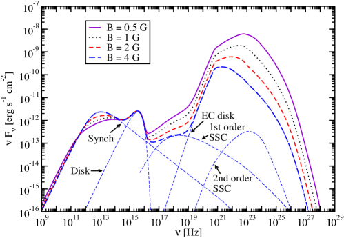
Figure 1.— Spectral energy distribution (SED) of accretion-disk/relativistic jet model using standard parameters for disk-jet system given by Table 1. Magnetic field is varied with the synchrotron flux remaining essentially constant, though with the peak synchrotron frequency varying between $\approx 2\times 10^{11}$ and $10^{13}$ eV. Separate spectral components (thin short dashed curves) are, from left to right, the synchrotron, accretion-disk, SSC, Compton-scattered accretion disk radiation, and second-order SSC components, for the high-magnetic field case, $B=4$ G.

The Compton-scattered accretion disk spectra are calculated from eq. (70). Fig. 1 shows the effects of changing the magnetic field. With increasing $B$, fewer electrons are required to make the same synchrotron flux, so that both the first and second-order SSC flux, and the flux of the Compton-scattered accretion-disk component decrease with increasing $B$. In all of these models, the second-order SSC emission is overwelmed by the external Compton component and is not visible. The overall levels of all Compton-scattered components are $\propto B^{-2}$.

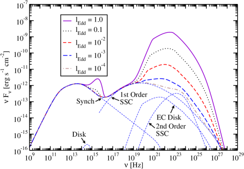
Figure 2.— Same as Fig. 1, except that the luminosity of the disk is changed. Separate spectral components are shown for the $l_{Edd}=10^{-4}$ case.

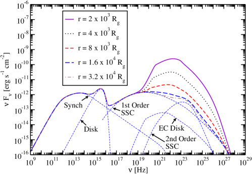
Figure 3.— Same as Fig. 1, except that the jet height is varied. Separate spectral components are shown for the $r=3.2\times 10^{4}\ R_{g}$ case.

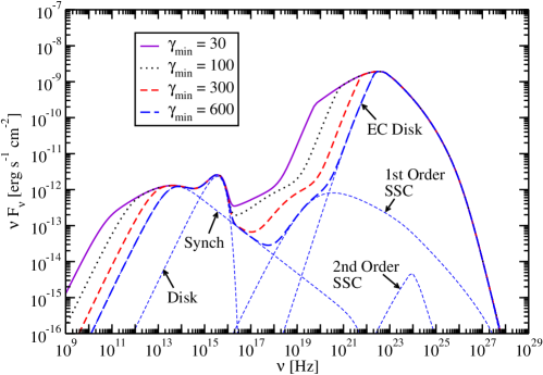
Figure 4.— Same as Fig. 1, except that the minimum electron Lorentz factor $\gamma^{\,\prime}_{min}$ is changed. Separate spectral components are shown for the $\gamma_{min}=600$ case.

With increasing disk power $\ell_{\rm Edd}$, the accretion-disk radiation and also the Compton-scattered accretion-disk component becomes progressively larger, as shown in Fig. 2. Note that the temperature of the disk photons at a given radius increases $\propto\ell_{\rm Edd}^{1/4}$. Fig. 3 displays the dependence of the blazar SED on height $\tilde{r}$ of the jet. As the blob’s distance from the disk increases, the level of the Comptonized disk radiation decreases. In both the case of changing the $\ell_{\rm Edd}$ and $\tilde{r}$ the SSC components are unaffected; eventually, the Compton-scattered disk flux falls below the SSC fluxes. The second-order SSC is visible when the external Compton flux decreases enough. Fig. 4 shows how variations in $\gamma_{min}$ affect the low energy part of the synchrotron, SSC, and external Compton components.

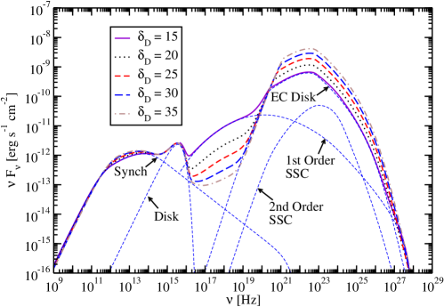
Figure 5.— Same as Fig. 1, except that the Doppler factor is varied with the synchrotron component essentially held constant. Separate spectral components are shown for the $\delta_{\rm D}=15$ case.

In Fig. 5, the Doppler factor is varied from the baseline value of 25, with the same approximate synchrotron flux. As $\delta_{\rm D}$ increases, the SSC component decreases, while the Compton-scattered accretion disk component increases. This behavior follows from eqs. (14) and (75), for the following reasons: For larger Doppler factors and fixed variability times, the radius becomes larger and fewer electrons are required to make the synchrotron flux at the same flux level, so the electron and internal photon energy densities decrease. Consequently the SSC flux decreases, but the larger value of $\delta_{\rm D}$ means that the external target photon field becomes more intense. Thus the Compton-scattered accretion disk radiation increases with increasing $\delta_{\rm D}$. Also, as the Doppler factor increases, the SSC component is shifted to lower energies while the Compton-disk component is shifted to higher energies, in accordance with eqs. (15) and (76), respectively.

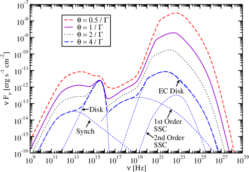
Figure 6.— Same as Fig. 1, except that the viewing angle is varied. The peak flux of the synchrotron, SSC, and near-field scattered disk component goes roughly as $\delta_{\rm D}^{4}$, $\delta_{\rm D}^{2}$, and $\delta_{\rm D}^{6}$, respectively. The different observing angles $\theta=1/\Gamma,2/\Gamma,3/\Gamma,4/\Gamma$ correspond to Doppler factors $\delta_{\rm D}=25,10,5,$ and 2.94, respectively. Separate spectral components are shown for the $\theta=4/\Gamma$ case.

Fig. 6 illustrates how the blazar SED is affected by changes in viewing angle. Contrary to Figs. (1) – (5), we let the synchrotron flux vary. In this calculation, $\Gamma=25$, and the observation angle and therefore $\delta_{\rm D}$ changes. It is interesting to note that the SSC flux varies least with changes in viewing angle, while the Comptonized disk component changes most rapidly. The ratios of the various components are explained by noting that $\delta_{\rm D}/\Gamma\cong 1,2/5,1/5,$ and 2/17 for $\theta\Gamma=1,2,3,$ and 4, respectively. The beaming factor for synchrotron radiation is $\propto\delta_{\rm D}^{3+\alpha}\propto\delta_{\rm D}^{4}$ in the flat portion of the $\nu F_{\nu}$ SED, with the convention that flux density $F_{\nu}\propto\nu^{-\alpha}$. The relative magnitudes of the SSC components are explained from eq. (14), noting that $f_{\epsilon_{pk}^{syn}}^{syn}\propto\delta_{\rm D}^{4}$, so that $f_{\epsilon_{pk}^{SSC}}^{SSC}\propto\delta_{\rm D}^{2}$. The peak flux of the scattered disk component in the near-field regime, $f_{\epsilon}^{ECNF}\propto\delta_{\rm D}^{6}$, from eq. (75).

A larger viewing angle or smaller Doppler factor implies a smaller size scale of the emitting region for a given variability time $t_{v}$. The characteristic Thomson scattering depth is $n^{\prime}_{e}\sigma_{\rm T}R^{\prime}_{b}\propto R^{\prime~{}-2}_{b}$ for a constant comoving electron spectrum $N^{\prime}_{e}(\gamma^{\,\prime})$ (described in our calculations by eq. [82]) in a region of size $R^{\prime}_{b}$. Consequently, the suppression of the SSC component due to Doppler boosting is offset by the increased scattering depth for larger observing angles.

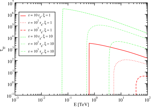
Figure 7.— Opacity of a photon emitted at various jet heights $\tilde{r}$ in units of $R_{g}$, subject to $\gamma\gamma$ pair production attenuation with photons from a Shakura-Sunyaev accretion disk with parameters given in Table 1. The parameter $\xi$ is defined in eq. (81).

Fig. 7 shows a calculation of the accretion-disk opacity $\tau_{\gamma\gamma}(\epsilon_{1},\tilde{r})$ for photons traveling along the jet axis, using eq. (80) and the parameters given in Table 1. Here we assume that the Shakura-Sunyaev disk reaches to the innermost stable orbit ($\tilde{R}_{i}=6$) of a Schwarzschild black hole. At larger jet heights, the accretion-disk opacity declines and only increasingly higher energy photons are subject to attenuation due to the threshold condition. The effect of increasing $\xi$ is to increase the mean accretion-disk photon energy at a given radius, from eq. (66), and therefore lower the energy at which $\gamma$ rays can be attenuated. At $\tilde{r}=10^{3}$, only $\gtrsim 10$ TeV photons are attenuated by the disk radiation field (with $\ell_{\rm Edd}=1$). The $\tau_{\gamma\gamma}$ corrections have not been included in the SED calculations, but are only important at $\nu\gtrsim 10^{25}$ Hz.

In all of our models the jet is particle-dominated ($P_{j,par}\gg P_{j,B}$) and the magnetic field is below its equipartition value. The total jet power, also divided into magnetic field and particle powers, is shown in Table 2. This is typical of results from modeling the observed X-ray and $\gamma$-ray emission of TeV blazars with the SSC component (Finke et al., 2008).

Table 2Jet Powers for Models in Figs. 1 – 6.

$B$ [G]	$\delta_{D}$	$\gamma_{min}$	$L_{B}$ [$10^{43}$ erg s-1]	$L_{par}$ [$10^{45}$ erg s-1]	$L_{tot}$ [$10^{45}$ erg s-1]
1	25	100	6.6	11	11
1	15	100	.85	36	36
1	20	100	2.7	19	19
1	30	100	14	7.5	7.6
1	35	100	25	5.3	5.5
0.5	25	100	1.6	27	27
2	25	100	26	4.8	5.0
4	25	100	110	2.0	3.1
1	25	30	6.6	18	18
1	25	300	6.6	5.7	5.7
1	25	600	6.6	3.0	3.0

3.3. External Isotropic Radiation Field

This is the case treated by Georganopoulos et al. (2001), where jet electrons scatter a surrounding external isotropic radiation field $u_{*}(\epsilon_{*},\Omega_{*})=u_{*}(\epsilon_{*})/4\pi$. By integrating eq. (28) over the angle variables, recognizing that $d\mu_{*}d\phi*=2\pi d\cos\psi$ for this geometry, one obtains

$$f^{{\rm C},iso}_{\epsilon}={3\over 4}\;{c\sigma_{\rm T}\epsilon_{s}^{2}\over 4\pi d_{L}^{2}}\;\delta_{\rm D}^{3}\;\int_{0}^{\infty}d\epsilon_{*}\;{u_{*}(\epsilon_{*})\over\epsilon_{*}^{2}}\int_{\gamma_{min}}^{\gamma_{max}}d\gamma\;{N^{\prime}_{e}(\gamma/\delta_{\rm D})\over\gamma^{2}}\;F_{\rm C}(q,\Gamma_{e})\;,$$ (84)

where $F_{\rm C}(q,\Gamma_{e})$ is given by Jones’s formula (Jones, 1968), eq. (7). Because the scattering is taking place in the stationary frame,

$$q\equiv{\epsilon_{s}/\gamma\over\Gamma_{e}(1-\epsilon_{s}/\gamma)}\;,$$ (85)

with $\Gamma_{e}=4\epsilon_{*}\gamma\;$ and, as before, $\epsilon_{s}=(1+z)\epsilon$. The limits $\gamma_{min}$ and $\gamma_{max}$ are given by

$$\gamma_{min}={1\over 2}\epsilon_{s}\;\left(1+\sqrt{1+{1\over\epsilon_{*}\epsilon_{s}}}\;\right)$$ (86)

and

$$\gamma_{max}={\epsilon_{*}\epsilon_{s}\over\epsilon_{*}-\epsilon_{s}}H(\epsilon_{*}-\epsilon_{s})\;+\;\gamma_{2}H(\epsilon_{s}-\epsilon_{*})\;.$$ (87)

For the case of the cosmic microwave background radiation (CMBR),

$${u_{*}(\epsilon_{*})\over 4\pi}\;=\;u_{bb}(\epsilon_{*},\Omega_{*})={2m_{e}c^{3}\over\lambda_{\rm C}^{3}}\;{\epsilon_{*}^{3}\over\exp(\epsilon_{*}/\Theta)-1}\;,$$ (88)

where $\Theta=k_{\rm B}T/m_{e}c^{2}$ is the dimensionless temperature of the blackbody radiation field, and $T=2.72(1+z)$ K. Substituting eq. (88) in eqs.  (22) and (33) gives

$$f_{\epsilon}^{{\rm C},CMBR}={3m_{e}c^{3}\sigma_{\rm T}\epsilon_{s}^{2}\delta_{\rm D}^{3}\over 2d_{L}^{2}\lambda_{\rm C}^{3}}\int_{0}^{\infty}d\epsilon_{*}\;{\epsilon_{*}\over\exp(\epsilon_{*}/\Theta)-1}\int_{\gamma_{min}}^{\gamma_{max}}d\gamma\;\gamma^{-2}N^{\prime}_{e}(\gamma/\delta_{\rm D})\;F_{\rm C}(q,\Gamma_{e})\;.$$ (89)

Eq. (89) gives an accurate spectrum of radiation made when jet electrons with number spectrum $N^{\prime}_{e}(\gamma^{\,\prime})$ Compton-scatter blackbody photons (see, e.g. Tavecchio et al., 2000; Dermer & Atoyan, 2002; Böttcher et al., 2008).

3.4. Scattered BLR Radiation Field

The BLR is thought to consist of dense clouds with a specified covering factor that can be determined from AGN studies. These clouds intercept central-source radiation to produce the broad emission lines in broad-line AGN (Kaspi & Netzer, 1999). The diffuse gas will also Thomson scatter the central source radiation. The scattered radiation provides an important source of target photons that jet electrons scatter to $\gamma$-ray energies (Sikora et al., 1994, 1997). This radiation field also attenuates $\gamma$ rays produced within the BLR (Blandford & Levinson, 1995; Levinson & Blandford, 1995; Böttcher & Dermer, 1995; Donea & Protheroe, 2003; Liu & Bai, 2006; Reimer, 2007; Sitarek & Bednarek, 2008).

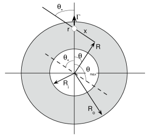
Figure 8.— Idealized geometry of the scattering region, approximated as a spherically-symmetric shell of gas with radial Thomson depth $\tau_{\rm T}$ between inner and outer radii $R_{i}$ and $R_{o}$, respectively, and a density gradient defined by index $\zeta$, where $n_{e}(R)\propto R^{\zeta}$.

Here we calculate the angular distribution of the Thomson-scattered radiation from a shell of gas with density

$$n_{e}(R)\;=n_{0}\left({R\over R_{i}}\right)^{\zeta}\;H(R;R_{i},R_{o})$$ (90)

extending from inner radius $R_{i}$ to outer radius $R_{o}$ (see Fig. 8; the calculation of fluorescence atomic-line radiation differs by considering dense clouds with a volume filling factor). The shell is assumed to be spherically symmetric with a power-law radial density distribution and radial Thomson depth $\tau_{\rm T}=\sigma_{\rm T}\int_{R_{i}}^{R_{o}}dR\;n_{e}(R)$. The Thomson-scattered spectral photon density can be estimated by noting that a fraction $\approx rn_{e}(r)\sigma_{\rm T}$ of the central source radiation with ambient photon density $n_{ph}(\epsilon_{*};r)=\dot{N}_{ph}(\epsilon_{*})/4\pi r^{2}c$ is scattered, giving a target scattered radiation field

$$n_{sc}(\epsilon_{*};r)\approx{n_{e}(r)\sigma_{\rm T}\dot{N}_{ph}(\epsilon_{*})\over 4\pi rc}\;$$ (91)

when $R_{i}\lesssim r\lesssim R_{0}$. Here $\dot{N}_{ph}(\epsilon_{*})=L(\epsilon_{*})/(m_{e}c^{2}\epsilon_{*})$ is the central source photon-production rate, assumed to radiate isotropically, and $L(\epsilon_{*})$ is its spectral luminosity.

A more accurate calculation of the Thomson-scattered photon density is obtained by integrating the expression

$$n_{ph}(\epsilon_{*};R)\;=\;\int dV\;{\dot{n}(\epsilon_{*};\vec{R})\over 4\pi x^{2}c}\;$$ (92)

over volume, where $dV=R^{2}d\phi d\mu dR$ and $x^{2}=R^{2}+r^{2}-2rR\cos\theta$ (Fig. 8). Assuming that the photons are isotropically Thomson-scattered by an electron without change in energy, so that $\dot{n}(\epsilon_{*};\vec{R})=\dot{N}_{ph}(\epsilon_{*})\sigma_{\rm T}n_{e}(R)/(4\pi R^{2}c)$, then

$$n_{ph}(\epsilon_{*};r)\;=\;{L(\epsilon_{*})\sigma_{\rm T}\over 8\pi m_{e}c^{3}\epsilon_{*}}\int_{-1}^{1}d\mu\;\int_{0}^{\infty}dR\;{n_{e}(R)\over x^{2}}\;=\;{L(\epsilon_{*})\sigma_{\rm T}\over 8\pi m_{e}c^{3}\epsilon_{*}r}\int_{0}^{\infty}dR\;{n_{e}(R)\over R}\;\ln\left|{R+r\over R-r}\right|$$ (93)

from a spherically-symmetric electron density distribution (cf. Gould, 1979; Böttcher & Dermer, 1995, for a time-dependent treatment). In the case of an isotropic, uniform surrounding medium, $n_{e}(R)=n_{0}$, $\zeta=0$, $R_{i}=0$ and $R_{o}\rightarrow\infty$ in eq. (90), and eq. (93) gives $n_{ph}(\epsilon_{*};r)=3.324\dot{N}_{ph}(\epsilon_{*})\sigma_{\rm T}n_{0}/(8\pi rc)$, noting that the integral $\int_{0}^{\infty}du\;\ln|(1+u)/(1-u)|/u\cong 3.324$. Thus the approximation given by eq. (91) is accurate to within a factor of $\approx 2$ for this case.

The angle-dependent scattered photon distribution $n_{ph}(\epsilon_{*},\mu_{*};r)$ can be derived by imposing a $\delta$-function constraint on the angle $\theta_{*}=\arccos\mu_{*}$ in eq. (92) (see also Donea & Protheroe, 2003), so that

$$n_{ph}(\epsilon_{*},\mu_{*};r)\;=\;{\sigma_{\rm T}\dot{N}_{ph}(\epsilon_{*})\over 8\pi cr}\;\int_{-\mu_{*}}^{1}d\mu\;\int_{0}^{\infty}dg\;{n_{e}(gr)\delta[\mu_{*}-\bar{\mu}_{*}(\mu,g)]\over g^{2}+1-2g\mu}\;,$$ (94)

after changing variables to $g=R/r$. From Fig. 8, $\theta_{max}=\pi-\theta_{*}$, so that $\mu_{min}=\cos\theta_{max}=\pi-\theta_{*}$ and $-\mu_{*}\leq\mu\leq 1$. The law of sines gives $R^{2}(1-\mu^{2})=x^{2}(1-\mu_{*}^{2})$, with the result

$$\bar{\mu}_{*}(\mu,g)\;=\;{\pm(1-g\mu)\over\sqrt{1+g^{2}-2g\mu}}\;.$$ (95)

Transforming the $\delta$-function in $\mu_{*}$ to a $\delta$-function in $g$ gives, after solving,

$$n_{ph}(\epsilon_{*},\mu_{*};r)\;=\;{\sigma_{\rm T}\dot{N}_{ph}(\epsilon_{*})\over 8\pi cr}\;{\cal N}(\mu_{*},r)\;,$$ (96)

where

$${\cal N}(\mu_{*},r)\;=\;{\cal N}[\mu_{*},n(r)]\;\equiv\;\int_{-\mu_{*}}^{1}d\mu\;n_{e}(\bar{g}r)\;{\sqrt{1+\bar{g}^{2}-2\bar{g}\mu}\over\bar{g}(1-\mu^{2})}\;$$ (97)

(units of ${\cal N}$ are $1/L^{3}$), and

$$\bar{g}\;=\;\bar{g}(\mu,\mu_{*})\;\equiv\;{-\mu(1-\mu_{*}^{2})+\mu_{*}\sqrt{(1-\mu^{2})(1-\mu_{*}^{2})}\over\mu_{*}^{2}-\mu^{2}}\;.$$ (98)

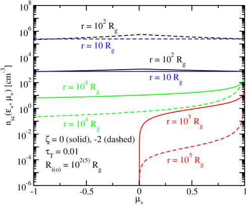
Figure 9.— Angle-dependent density of Thomson-scattered radiation at height $r$ along the jet axis. The radial Thomson depth of the spherically-symmetric scattering medium is $\tau_{\rm T}=0.01$, and the scattering shell is assumed to extend from $10^{2}$ to $10^{5}$ Schwarzschild radii for a $10^{8}M_{\odot}$ black hole. The solid and dashed curves show results with $\zeta=0$ and $\zeta=-2$, respectively. The values of $r$ for are labeled on the dashed curves. The ratio of the luminosity of the photon source to the dimensionless photon energy is $L_{*}/\epsilon_{*}=10^{44}$ ergs s^-1, and the calculation assumes that $\epsilon_{*}\ll 1$, so that scattering is in the Thomson regime (see eq. [99]).

Fig. 9 shows the angle dependence of the scattered radiation field in the stationary frame for this idealized geometry for the parameters given in the figure caption. As can be seen, the scattered radiation field is nearly isotropic when $r<R_{i}$, and starts to display increasing asymmetry peaked in the outward direction at increasingly greater heights. When $r>R_{o}$, all scattered radiation is outwardly directed. Most of the scattering material is near the inner edge when $\zeta=-2$, so that the intensity of the scattered radiation field is largest at $r\lesssim R_{i}$. By contrast, the intensity of the scattered radiation field is not so enhanced towards the inner regions when $\zeta=0$.

The Compton-scattered radiation spectrum is given, in general, by eq. (34). Substituting eq. (96) for the angular distribution of the target photon source gives, for a monochromatic photon source

$$\dot{N}_{ph}(\epsilon_{*})={L_{0}\delta(\epsilon_{*}-\epsilon_{*0})\over m_{e}c^{2}\epsilon_{*}}\;,$$ (99)

the $\nu F_{\nu}$ flux

$$f_{\epsilon}^{EC,scat}(r)\;=\;{(\pi r_{e}^{2})^{2}L_{0}\delta_{\rm D}^{3}\over 12\pi^{2}d_{L}^{2}r}\;\left({\epsilon_{s}\over\epsilon_{*}}\right)^{2}\;\int_{\max(-1,1-2\epsilon_{s}/\epsilon_{*})}^{1}d\mu_{*}\;{\cal N}(\mu_{*},r)\;\int_{\tilde{\gamma}_{low}}^{\infty}d\gamma\;{N_{e}^{\prime}(\gamma/\delta_{\rm D})\over\gamma^{2}}\;\Xi\;.$$ (100)

In this expression,

$$\tilde{\gamma}_{low}\;\equiv\;{\epsilon_{s}\over 2}\;\left[1+\sqrt{1+{2\over\epsilon_{*}\epsilon_{s}(1-\mu_{*})}}\;\right]\;$$ (101)

(compare eq. [29]). Substituting eq. (96) into eq. (20) for a monochromatic photon source, eq. (99), gives

$$\tau_{\gamma\gamma}(\epsilon_{1},r)\;=\;{\sigma_{\rm T}L_{0}\over 8\pi m_{e}c^{3}\epsilon_{*}}\;\int_{r}^{\infty}{dx\over x}\;\int_{-1}^{1-2/[\epsilon_{1}\epsilon_{*}(1+z)]}d\mu_{*}\;(1-\mu_{*})\;{\cal N}(\mu_{*},x)\sigma_{\gamma\gamma}(s)\;$$ (102)

for the opacity of a photon with measured energy $\epsilon_{1}$ emitted outward along the jet axis at height $r$. The $\gamma\gamma$ opacity vanishes when $\epsilon_{1}\leq 1/[\epsilon_{*}(1+z)]$ due to the $\gamma\gamma$ pair-production threshold.

3.4.1 Thomson-Scattered Isotropic Monochromatic Radiation Field

Substituting $u_{*}(\epsilon_{*},\Omega_{*})=u_{*0}\delta(\epsilon_{*}-\epsilon_{*0})/4\pi$ for an isotropic monochromatic radiation field in eq. (35) gives, with $\Xi\rightarrow 2$ for the Thomson regime away from the endpoints of the spectrum,

$$f_{\epsilon}^{{\rm T},iso}={c\pi r_{e}^{2}\delta_{\rm D}^{3+p}u_{*0}\over 4\pi d_{L}^{2}}\;\left({\epsilon_{s}\over\epsilon_{*}}\right)^{2}\;\int_{\max(-1,1-2\epsilon_{s}/\epsilon_{*})}^{1}d\mu_{*}\;\int_{\sqrt{\epsilon_{s}/2\epsilon_{*}(1-\mu_{*})}}^{\infty}d\gamma\;\gamma^{-2}N_{e}^{\prime}(\gamma/\delta_{\rm D})\;.$$ (103)

We consider Compton up-scattering, i.e., $\epsilon_{s}>\epsilon_{*}$ for the power-law electron spectrum given by eq. (47). The Thomson approximation is only valid far from the endpoints. The asymptotes for the Thomson-scattered spectrum of a surrounding isotropic, monochromatic radiation field therefore becomes

$$f_{\epsilon}^{{\rm T},iso}\cong{2c\pi r_{e}^{2}u_{*0}\over 4\pi d_{L}^{2}(p+1)}\;K^{\prime}\left({\epsilon_{s}\over\epsilon_{*}}\right)^{2}\;\delta_{\rm D}^{2}\gamma_{1}^{\prime~{}-(p+1)}\;,\;{\rm for}\;\;\epsilon_{*}\lesssim\epsilon_{s}\ll 4\epsilon_{s}(\delta_{\rm D}^{2}\gamma_{1}^{\prime})^{2}\;,$$ (104)

and

$$f_{\epsilon}^{{\rm T},iso}\cong{2^{p+3}\over(p+1)(p+3)}\;{c\pi r_{e}^{2}\delta_{\rm D}^{3+p}u_{*0}\over 4\pi d_{L}^{2}}\;K^{\prime}\left({\epsilon_{s}\over\epsilon_{*}}\right)^{(3-p)/2}\;,\;{\rm for}\;\;4\epsilon_{s}(\delta_{\rm D}^{2}\gamma_{1}^{\prime})^{2}\lesssim\epsilon_{s}\ll 4\epsilon_{s}(\delta_{\rm D}^{2}\gamma_{2}^{\prime})^{2}\;.$$ (105)

Note the different beaming factors in the two asymptotes. Eq. (105) agrees with the Thomson expression derived by Dermer et al. (1997), eq. (22), to within factors of order unity.

3.4.2 Numerical Calculations

We now present calculations of the SED of FSRQ blazars, including the external Compton-scattering component formed by jet electrons that scatter target photons which themselves were previously scattered by BLR material. This EC BLR component is not found in conventional synchrotron/SSC models of blazars, and so distinguishes standard model blazar BL Lacs and FSRQs. The inclusion of the $\gamma\gamma$ opacity through the scattered radiation makes the calculation self-consistent.

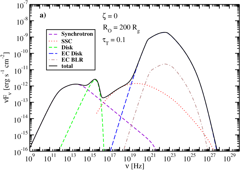
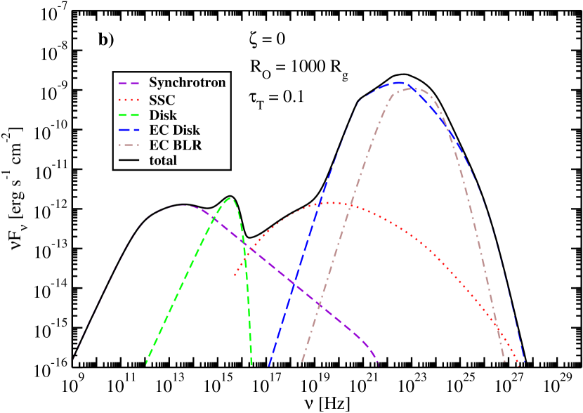
Figure 10.— Standard model FSRQ blazar with standard parameters given in Table 1. The optical depth through the BLR is $\tau_{\rm T}=0.1$, with no gradient in the density of the scattering material. The radiating jet is located at $10^{3}R_{g}$. Separate synchrotron, accretion-disk, SSC, EC Disk, and EC BLR components are shown. (a) The BLR extends from $100$ to $200R_{g}$. (b) The BLR extends from $100$ to $1000R_{g}$.

For the simplified shell geometry depicted in Fig. 8, we calculate the external Compton scattering component using eq. (100), and calculate the $\gamma\gamma$ opacity using eq. (102). To simplify the calculations, the spectrum of the radiation scattered by the BLR is assumed to be monochromatic with energy $\approx 50$ eV, corresponding to the mean energy from the accretion-disk radiation for the standard model. Results of such a calculation are shown in Fig. 10, using parameters for a standard FSRQ blazar model given in Table 1. The constant-density BLR is confined between 100 and 200 $R_{g}$, and the Thomson depth through the BLR is $\tau_{\rm T}=0.1$. In Fig. 10(a), the emission region of the jet is far outside the BLR, at 1000 $R_{g}$. Therefore most of the BLR photons encounter the jet from behind, and the rate of tail-on scatterings is suppressed by the rate factor. Consequently, the flux of the EC BLR component is much less that the flux of the EC Disk component. Fig. 10(b) presents a similar calculation, except that the BLR now extends to $10^{3}R_{g}$, the same radius where the radiating jet is assumed to be located. As expected, the EC BLR component is significantly enhanced compared to Fig. 10(a).

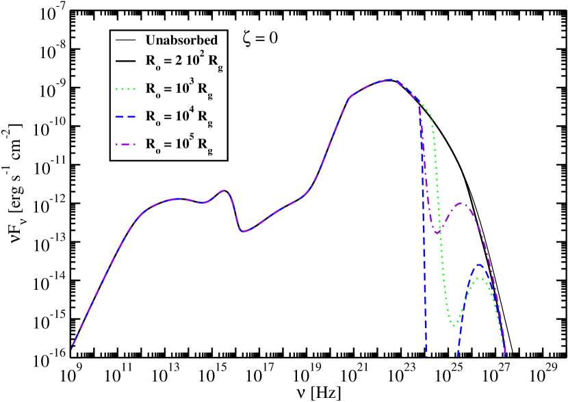
Figure 11.— Model blazar SED comprised of synchrotron, accretion-disk, SSC, EC disk, and EC BLR components, including $\gamma\gamma$ attenuation by the scattered BLR radiation. The jet height $r=10^{3}R_{g}$. The outer radius, $R_{o}$, of the BLR is varied, keeping its Thomson depth, $\tau_{\rm T}=0.01$, constant.

There is very little $\gamma\gamma$ absorption by the accretion-disk radiation or the BLR radiation when the jet is found outside the BLR. On the other hand, when the jet is within the BLR, there can be significant $\gamma\gamma$ opacity. This is shown in Fig. 11, where we use the standard parameters for the jet and a BLR with $\tau_{\rm T}=0.01$, except that the outer radius, $R_{o}$, of the BLR is varied. The effects of $\gamma\gamma$ attenuation by the scattered radiation field are shown. When $R_{o}<<r$, the jet height, then the threshold is suppressed except for the highest-energy $\gamma$ rays. When the blob lies within the BLR, $r\lesssim R_{o}$, the opacity from the scattered BLR radiation is significant and the $\gamma\gamma$ opacity large for $\gamma$ rays with $\epsilon\sim 2/\epsilon_{*}$, which for our monochromatic radiation field with $\epsilon_{*}\cong 10^{-4}$, is at $\nu\sim 5\times 10^{24}$ Hz ($\approx 40$ GeV). When $R_{o}\gg r$, the $\gamma\gamma$ opacity, proportional to $rn_{sc}(\epsilon_{*};r)$, declines $\propto R_{0}^{-1}$ for constant Thomson depth, as can be seen from eq. (91). Note that the EC $\gamma$ rays are not very sensitive to the changes in the BLR parameters, since most of the emission is formed by the EC disk component.

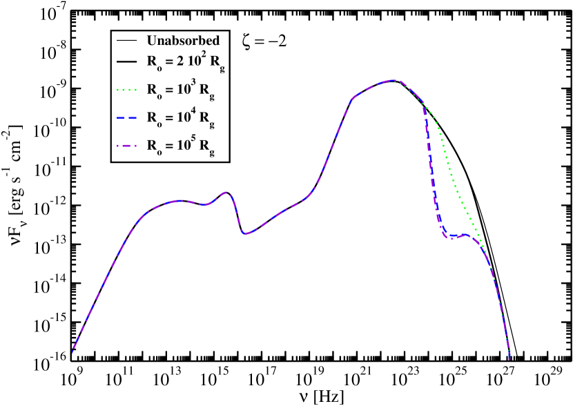
Figure 12.— Same as Fig. 11, except that the gradient $\zeta=-2$ in the density distribution.

The effect of changing the radial gradient of BLR scattering material is shown in Fig. 12. For a steeper density gradient, $\zeta=-2$, and a constant Thomson depth, the material is concentrated near the inner edge of the BLR at $R_{i}$, so the changes in the $\gamma\gamma$ opacity are most dramatic when $R_{o}\approx r$ due to geometric effects. When $R_{i}\ll r\ll R_{o}$, the radiation field is essentially unchanged for different values of $R_{o}$, and so also is the $\gamma\gamma$ opacity.

4. Discussion and Summary

We have presented accurate expressions for modeling synchrotron and Compton-scattered radiation from the jets of AGN that include target radiation fields from the accretion disk and BLR. This extends our technique for modeling synchrotron and SSC emission (Finke et al., 2008) to include external Compton scattering in a relativistic jet of thermal radiation from the accretion disk, and accretion-disk radiation Thomson-scattered by electrons in the BLR. These formulae use the full Compton cross section and are accurate throughout the Thomson and Klein-Nishina regimes at any angle with respect to the jet axis, so can also be used to model $\gamma$-ray emission from radio galaxies, e.g., M87 (Aharonian et al., 2006). We also derive expressions for the $\gamma\gamma$ opacity through the same scattered radiation field that serves as a target photon source for the jet electrons. The expressions, eqs. (80) and (102), for opacity from the accretion-disk and scattered radiation field assume, however, that the photon travels along the jet axis, though it is straightforward to derive the more general case.

In the results presented here (Figs. 1 – 6 and 10 – 12) we have chosen parameters for demonstration purposes that give an exaggerated EC component, particularly a high $\ell_{\rm Edd}$. Lowering the disk luminosity lowers the radiation considerably, as seen in Fig. 2. The disk radiation field in FSRQ blazars can be seen when the nonthermal blazar radiation is in a low state, as in the cases of 3C 279 (Pian et al., 1999), 3C 454.3 (Raiteri et al., 2007) and, most clearly, 3C 273 (e.g., von Montigny et al., 1997). These observations can be used to assign the accretion-disk luminosity when modeling a specific blazar, though the disk brightness could also vary during the flaring epoch.

The models presented here do, however, have limitations. They do not yet include enhancements from secondary cascade radiation initiated by $e^{\pm}$ pairs formed by $\gamma$ rays interacting with lower energy radiation from the disk and the BLR. For the parameters considered here, this would not make a significant difference in the calculated SEDs because the energy flux of the attenuated radiation is a small fraction of the escaping flux. But even in this case, the reinjected pairs from the attenuated radiation will be isotropized if the reinjection occurs outside the relativistic flow, and will then make only a small contribution to the Doppler-boosted radiation.

Spectral features result from $\gamma\gamma$ absorption by BLR radiation, as seen in Fig. 12. By assuming hard primary $\gamma$-ray emission components, Aharonian et al. (2008) argue that hard intrinsic spectra from blazars such as 1ES 1101-232 (Aharonian et al., 2007b) could be formed through $\gamma\gamma$ attenuation. If the primary TeV radiation originates from an underlying jetted electron distribution, then a consistent model requires that a $\gamma$-ray spectrum formed by Compton-scattering processes arises from the same radiation field responsible for $\gamma\gamma$ absorption. As our calculations show, soft Compton-scattered TeV spectra are formed due to Klein-Nishina effects in scattering, whether from the accretion disk or from photons scattered by the BLR. Thus either an extremely bright GeV component would be expected in the scenario of Aharonian et al. (2008) (cf. Figs. 11 and 12), which would easily be detected with Fermi, or a hard primary $\gamma$-ray spectrum must originate from other processes. Moreover, if this explanation was correct, then blazars with stronger broad emission lines should have harder VHE $\gamma$-ray spectra than weak-lined BL Lacs.

Cascade radiation induced by ultra-relativistic hadrons could inject high-energy leptons to form a hard radiation component, though a sufficiently dense target field for efficient photohadronic losses will itself severely attenuate the TeV radiation (Atoyan & Dermer, 2003). Depending on the underlying acceleration model, a distinctive hadronic signature could appear at $\gamma$-ray energies only, though one would expect that both electrons and protons would be accelerated synchronously.

Our calculations also do not as yet include absorption by the diffuse extragalactic background light (EBL), which would be important for EGRET $\gamma$-ray FSRQs, which have a broad redshift distribution with a mean value $\langle z\rangle\sim 1$, larger than the mean value $\langle z\rangle\sim 0.3$ for BL Lacs (Mukherjee et al., 1997). In cases where the Compton-scattered spectra decline steeply due to Klein-Nishina effects (e.g., Fig. 1), the issue of EBL absorption is secondary. In the one FSRQ, 3C 279 (catalog ) at $z=0.536$, detected from 80 to $>300$ GeV energies with MAGIC (MAGIC Collaboration, 2008), EBL effects cannot be neglected. For the models studied here, the soft calculated $\gamma$-ray spectra cannot in any case account for the measured, let alone intrinsic, spectrum of 3C 279. Based on the simultaneous optical – X-ray – VHE $\gamma$-ray SED of 3C279 during the MAGIC detection, Böttcher, Marscher & Reimer (2008, in preparation) show that one-zone leptonic models have severe problems explaining the flare, and require either extremely high Doppler factors or magnetic fields well below equipartition. Correlated X-ray, Fermi, and TeV campaigns will offer opportunities to apply the results developed in this paper.

In conclusion, we have derived expressions to model FSRQ blazars that self-consistently include $\gamma\gamma$ attenuation on the same target photons that are Compton-scattered by the relativistic electrons. By assuming that the lower energy, radio – UV emission is nonthermal synchrotron radiation, then the underlying electron distribution can be determined given the Doppler factor, magnetic field, and size scale of the emission region. The equations derived here can be used to calculate the $\gamma$-ray emission spectrum from SSC and external Compton scattering processes from this electron distribution. Separately, one can determine whether the inferred electron distribution can be derived from specific acceleration scenarios. Complementary to the technique of injecting electron spectra and cooling, this method can be applied to multiwavelength data sets to analyze high-energy processes in the jets of AGN.

References

- Aharonian et al. (2006) Aharonian, F., Akhperjanian, A. G., Bazer-Bachi, A. R., & et al. 2006, Science, 314, 1424
- Aharonian et al. (2007b) Aharonian, F., et al. 2007b, A&A, 470, 475
- Aharonian et al. (2008) Aharonian, F. A., Khangulyan, D., & Costamante, L. 2008, MNRAS, 387, 1206
- Atoyan & Dermer (2003) Atoyan, A. M., & Dermer, C. D. 2003, ApJ, 586, 79
- Band et al. (1993) Band, D., et al. 1993, ApJ, 413, 281
- Becker & Kafatos (1995) Becker, P. A., & Kafatos, M. 1995, ApJ, 453, 83
- Blandford & Levinson (1995) Blandford, R. D., & Levinson, A. 1995, ApJ, 441, 79
- Błażejowski et al. (2000) Błażejowski, M., Sikora, M., Moderski, R., & Madejski, G. M. 2000, ApJ, 545, 107
- Bloom & Marscher (1996) Bloom, S. D., & Marscher, A. P. 1996, ApJ, 461, 657
- Blumenthal & Gould (1970) Blumenthal, G. R., & Gould, R. J. 1970, Reviews of Modern Physics, 42, 237
- Böttcher et al. (2008) Böttcher, M., Dermer, C. D., & Finke, J. D. 2008, ApJ, 679, L9
- Böttcher & Dermer (1995) Böttcher, M., & Dermer, C. D. 1995, A&A, 302, 37
- Böttcher & Bloom (2000) Böttcher, M., & Bloom, S. D. 2000, AJ, 119, 469
- Böttcher et al. (1997) Böttcher, M., Mause, H., & Schlickeiser, R. 1997, A&A, 324, 395
- Böttcher & Reimer (2004) Böttcher, M., & Reimer, A. 2004, ApJ, 609, 576
- Brown, Mikaelian, & Gould (1973) Brown, R. W., Mikaelian, K. O., & Gould, R. J. 1973, Astrophys. Lett. 14, 203