Dvali-Gabadadze-Porrati Cosmology in Bianchi I brane

Abstract

The dynamics of Dvali-Gabadadze-Porrati Cosmology (DGP) braneworld with an anisotropic brane is studied. The Friedmann equations and their solutions are obtained for two branches of anisotropic DGP model. The late time behavior in DGP cosmology is examined in the presence of anisotropy which shows that universe enters a self-accelerating phase much later compared to the isotropic case. The acceleration conditions and slow-roll conditions for inflation are obtained.

I Introduction

Cosmological models inspired by higher dimensional theories have received a lot of attention in recent times. In these models our observed four-dimensional (4D) universe is a three dimensional hypersurface (brane) embedded in a higher dimensional space-time called bulk (for a review see brax ). Two popular cosmological models emerging out of higher dimensional theories are Randall-Sundrum (RS) lisa and the Dvali-Gabadadze-Porrati (DGP) model dvali . The generalisation of such models to the homogenious and isotropic Friedmann-Robertson-Walker (FRW) brane leads to modification of the Friedmann equation with a quadratic correction to energy density at higher energies. Many issues in cosmology like inflation, dark energy, cosmological constant were investigated in the braneworld cosmological scenario and encouraging results were obtained.

Although the present universe appears homogeneous and isotropic in its overall structure, as indicated from recent WMAP data that cosmic microwave background is isotropic up to 1 part in $10^{5}$. But there are reasons to believe that it has not been so in all its evolution and that inhomogeneities and anisotropies played an important role in the early universe. There exists a large number of anisotropic cosmological models, which are also being studied in cosmology, due to various reasons mis .

Hence, it is natural to ask how these anisotropies play a role in the context of the braneworld scenario. The anisotropic braneworld with a scalar field is studied in varun and it is shown that a large initial anisotropy introduces more damping in the scalar field equation of motion resulting in greater inflation. Cosmological solutions for the Bianchi-I and Bianchi-V in the case of the RS branemodel were studied in camp . It is shown that for matter on the brane obeying the bariotropic equation of state, the anisotropic Bianchi-I,V braneworlds always isotropise although there could be intermediate stages in which anisotropy grows. The shear dynamics in the Bianchi-I brane model were studied in top and shown that for $1<\gamma<2$ shear has maximum value during the phase transition from nonstandard to standard cosmology. The cosmological solution of field equations for an anisotropic brane in the generalised RS model were obtained in pal and the solution admits an inflationary era. Dissipation of anisotropy on the brane is explicitly demonstrated by the particle production mechanism in gus by considering the Bianchi-I braneworld model. Apart from this there have been studies frolov which show that anisotropy plays an important role in braneworld models. All the previous studies have mainly focussed on anisotropy on the Randall-Sundrum braneworld.

In this paper we consider the DGP braneworld model with anisotropy and find a solution of field equations. The DGP cosmological model possesses two classes of solutions; one which is close to standard FRW cosmology and the other is a fully five dimensional regime or a self-inflationary solution which produces accelerated expansion. It is also noted in ant that the self-accelerating universe exhibit ghost and tachyonic like excitations. We are mainly interested in effects of initial anisotropy and show that it is possible to get self-inflationary solution in the presence of anisotropy. We also explore an acceleration condition for the DGP cosmological model with a scalar field dominated universe, in the presence of shear.

II Field equations in the DGP model

We consider the DGP model, where our universe is a 3-brane embedded in 5D bulk with an infinite size extra dimension and there is an induced 4D Ricci scalar on the brane, due to radiative correction to the graviton propagator on the brane. In this model there exists a length scale below which the potential has usual Newtonian form and above which the gravity becomes five dimensional. The crossover scale between the four-dimensional and five-dimensional gravity is given by,

$$r_{c}=\frac{k_{5}^{2}}{2\mu^{2}}$$ (1)

where $\mu^{2}=8\pi G_{4}$ and $k^{2}_{5}=8\pi G_{5}$ are the constants related to 4D and 5D Newton’s constants respectively. The Einstein equation for a five dimensional bulk is given by,

$$G_{AB}=-\Lambda g_{AB}+k_{5}^{2}(T_{AB}+S_{AB}\delta(y)),$$ (2)

where $\Lambda$ is the bulk cosmological constant, $T_{AB}$ is the five-dimensional energy momentum tensor (A,B = 0,..4 ) and $S_{AB}$ is the 4D energy-momentum tensor and is given by,

$$S_{AB}=\tau_{AB}-\sigma q_{AB}-\mu^{-2}G_{AB},$$ (3)

where $\tau_{AB}$ is the energy-momentum tensor of matter fields on the brane, $\sigma$ is the brane tension, and the last term in the above equation represents contribution from the induced curvature term. Assuming $Z_{2}$ symmetry for the brane and using the Israel junction condition, the effective Einstein equation on the brane is obtained as sas ; riz ,

$$\left(1+\frac{\sigma k^{2}_{5}}{6\mu^{2}}\right)G_{\mu\nu} = -\left(\frac{k^{2}_{5}\Lambda}{2}+\frac{k^{4}_{5}\sigma^{2}}{12}\right)q_{\mu\nu}+\mu^{2}T_{\mu\nu}$$ (4)

$$+\frac{\sigma k^{4}_{5}}{6}\tau_{\mu\nu}+\frac{k^{4}_{5}}{\mu^{4}}F_{\mu\nu}+k^{4}_{5}\Pi_{\mu\nu}+\frac{k^{4}_{5}}{\mu^{2}}L_{\mu\nu}-E_{\mu\nu},$$

$$\Pi_{\mu\nu}=-\frac{1}{4}\tau_{\mu\rho}\tau^{\rho}_{\nu}+\frac{1}{12}\tau\tau_{\mu\nu}+\frac{1}{8}q_{\mu\nu}\tau_{\alpha\beta}\tau^{\alpha\beta}-\frac{1}{24}q_{\mu\nu}\tau^{2},$$ (5)

$$F_{\mu\nu}=-\frac{1}{4}G_{\mu\rho}G^{\rho}_{\nu}+\frac{1}{12}GG_{\mu\nu}+\frac{1}{8}q_{\mu\nu}G_{\alpha\beta}G^{\alpha\beta}-\frac{1}{24}q_{\mu\nu}G^{2},$$ (6)

$$L_{\mu\nu}=\frac{1}{4}(G_{\mu\rho}\tau^{\rho}_{\nu}+\tau_{\mu\rho}G^{\rho}_{\nu})-\frac{1}{12}(\tau G_{\mu\nu}+G\tau_{\mu\nu})-\frac{1}{4}q_{\mu\nu}(G_{\alpha\beta}\tau^{\alpha\beta}-\frac{1}{3}G\tau),$$ (7)

where $T_{\mu\nu}$ is the bulk energy-momentum tensor. It is noticed that in Eq. (4), apart from the usual quadratic matter field corrections to energy momentum, there are corrections coming from the induced curvature term through $F_{\mu\nu}$ and $L_{\mu\nu}$. $E_{\mu\nu}$ is the projection of the bulk Weyl tensor on the brane representing the nonlocal effects from the free gravitational field. If we define the four velocity comoving with matter as $u_{\mu}$ hawk , the non-local term takes the form,

$$E_{\mu\nu}=-4r_{c}^{2}[U(u_{\mu}u_{\nu}+\frac{1}{3}h_{\mu\nu})+P_{\mu\nu}+Q_{\mu}u_{\nu}+Q_{\nu}u_{\mu}].$$ (8)

where $h_{\mu\nu}=g_{\mu\nu}+u_{\mu}u_{\nu}$ and

$$U=-\frac{1}{4r_{c}^{2}}E_{\mu\nu}u^{\mu}u^{\nu},$$ (9)

is an effective nonlocal energy density on the brane,

$$P_{\mu\nu}=-\frac{1}{4r_{c}^{2}}\left[h_{\mu}{}^{\alpha}h_{\nu}{}^{\beta}-{\textstyle{1\over 3}}h^{\alpha\beta}h_{\mu\nu}\right]E_{\alpha\beta}$$ (10)

is the effective nonlocal anisotropic stress, and

$$Q_{\mu}=\frac{1}{4r_{c}^{2}}h_{\mu}{}^{\alpha}E_{\alpha\beta}u^{\beta}\,,$$ (11)

represents the effective nonlocal energy flux on the brane.

At this stage we set the bulk cosmological constant, brane tension to zero and consider empty bulk, then Eq. (4) becomes,

$$G_{\mu\nu}=\frac{k^{4}_{5}}{\mu^{4}}F_{\mu\nu}+k^{4}_{5}\Pi_{\mu\nu}+\frac{k^{4}_{5}}{\mu^{2}}L_{\mu\nu}-E_{\mu\nu}.$$ (12)

We combine all the nonlocal and local bulk corrections and these can be written in an compact form as,

$$G_{\mu\nu}=k^{4}_{5}T^{\rm tot}_{\mu\nu}\,,$$ (13)

where,

$$T^{\rm tot}_{\mu\nu}=\frac{1}{\mu^{4}}F_{\mu\nu}+\Pi_{\mu\nu}+\frac{1}{\mu^{2}}L_{\mu\nu}-{1\over k^{4}_{5}}E_{\mu\nu}\,.$$ (14)

Following mar the effective energy density, pressure, anisotropic stress, and energy density, for the DGP case can be calculated and are obtained as,

$$\rho_{\rm tot}=\frac{1}{12}\left(\rho^{2}-\frac{2}{\mu^{2}}G_{00}\rho+\frac{1}{\mu^{4}}G_{00}^{2}\right)+\frac{4r_{c}^{2}}{k^{4}_{5}}U,$$ (15)

$$p_{\rm tot}=\frac{1}{12}\left(\rho(\rho+2p)-\frac{2}{\mu^{2}}G_{00}(\rho+p)-\frac{2}{\mu^{2}}G_{ii}\rho+\frac{1}{\mu^{4}}G_{00}(G_{00}+2G_{ii})\right)+\frac{4r_{c}^{2}}{3k^{4}_{5}}U,$$ (16)

$$\pi^{\rm tot}_{\mu\nu}=\frac{4r_{c}^{2}}{k^{4}_{5}}P_{\mu\nu},$$ (17)

$$q^{\rm tot}_{\mu}=\frac{4r_{c}^{2}}{k^{4}_{5}}Q_{\mu}.$$ (18)

It is assumed that the total energy-momentum tensor and the brane energy-momentum tensor are conserved independently mar . It can be seen from Eqs. (8-11) that results depend on the crossover scale $r_{c}$ of the theory, which is a typical feature of the DGP model. When $r_{c}$ goes to zero the effective nonlocal energy density, anisotropic stress, and energy flux diverge.

III DGP Cosmology on a Bianchi-I brane

We consider an anisotropic Bianchi-I brane model with the metric given by,

$$ds^{2}=-dt^{2}+a_{i}^{2}(t)(dx^{i})^{2}\,,$$ (19)

and is covariantly characterized by varun

$$D_{\mu}f=0\,,~{}A_{\mu}=0=\omega_{\mu}\,,~{}Q_{\mu}=0\,,~{}R^{*}_{\mu\nu}=0\,,$$ (20)

where $D_{\mu}$ is the projected covariant spatial derivative, $f$ is any physical defined scalar, $A_{\mu}$ is the four acceleration, $\omega_{\mu}$ is the vorticity and $R^{*}_{\mu\nu}$ is the Ricci tensor of the three surface orthogonal to $u_{\mu}$.

The conservation equations takes the following form:

$$\dot{\rho}+\Theta(\rho+p)=0$$ (21)

$$D^{\nu}P_{\mu\nu}=0$$ (22)

$$\dot{U}+{\textstyle{4\over 3}}\Theta{U}+\sigma^{\mu\nu}{P}_{\mu\nu}=0$$ (23)

where the dot denotes the $u^{\nu}\nabla_{\nu}$ and $\Theta$ represents the volume expansion rate and $\sigma^{\mu\nu}$ is the shear rate. The Hubble parameter for the Bianchi-I metric is given by $H_{i}=\frac{{\dot{a}_{i}}}{a_{i}}$ and one can define the mean expansion factor as $S=(a_{1}a_{2}a_{3})^{1/3}$, thus

$$\Theta\equiv 3H=3\frac{{\dot{S}}}{S}\equiv\sum_{i}H_{i}.$$ (24)

The Raychaudhuri equation for the Bianchi-I metric on the brane is obtained as,

$$\dot{\Theta}+\frac{1}{3}\Theta^{2}+\sigma^{\mu\nu}\sigma_{\mu\nu} = \frac{-k^{2}_{5}}{2}\left[\frac{1}{12\mu^{4}}\left(3\left({H^{2}+\frac{K}{S^{2}}}\right)-\mu^{2}\rho\right)^{2}+\frac{1}{4}\rho(\rho+2p)\right.$$ (25)

$$\left.-\frac{1}{2\mu^{2}}\left(3\left({H^{2}+\frac{K}{S^{2}}}\right)(\rho+p)+G_{ii}\rho\right)\right.$$

$$\left.+\frac{1}{4\mu^{4}}3\left(H^{2}+\frac{K}{S^{2}}\right)\left(3\left(H^{2}+\frac{K}{S^{2}}\right)+2G_{ii}\right)+\frac{8r_{c}^{2}}{k^{4}_{5}}U\right].$$

and Gauss-Codacci equations are

$$\dot{\sigma}_{\mu\nu}+\Theta\sigma_{\mu\nu}=4r_{c}^{2}P_{\mu\nu}\,$$ (26)

$$\frac{2}{3}\Theta^{2}+\sigma^{\mu\nu}\sigma_{\mu\nu}=\frac{k^{4}_{5}}{6\mu^{4}}\left(3\left(H^{2}+\frac{K}{S^{2}}\right)-\mu^{2}\rho\right)^{2}+4r_{c}^{2}U\,.$$ (27)

It is noticed that there is no evolution equation for $P_{\mu\nu}$, indicating the fact that in general the equations do not close on the brane and complete bulk equations are needed to determine the brane dynamics. There are bulk degrees of freedom whose impact cannot be predicted by brane observers. Hence, the presence of $P_{\mu\nu}$ in Eq. (26) does not allow us to simply integrate to get the value of shear as in general relativity. We can overcome this problem by considering a special case where nonlocal energy density vanishes or is negligiblevarun i.e. $U=0$, which is often assumed for FRW branes and leads to conformally flat bulk geometry. Under this assumption conservation Eq. (23) leads to $\sigma_{\mu\nu}P^{\mu\nu}=0$; this consistency condition implies a condition on evolution of $P_{\mu\nu}$ as $\sigma^{\mu\nu}\dot{{P}_{\mu\nu}}=4r_{c}^{2}P^{\mu\nu}P_{\mu\nu}$, folowing from Eq. (26). As there is no evolution equation for $P_{\mu\nu}$ on the brane mar ; varun , this is consistent on the brane. Also, one should check that the brane metric with $U=0$ leads to a physical 5D bulk metric. This has to be done numerically as the bulk metric for the Bianchi brane is not known and is beyond the scope of the present paper.

Now Eq. (26) can be integrated after contracting with shear varun and gives

$$\sigma^{\mu\nu}\sigma_{\mu\nu}=2\sigma^{2}={6\Sigma^{2}\over S^{6}}\,,~{}~{}\dot{\Sigma}=0\,.$$ (28)

Figure 1: Evolution of scalar factor with and without anisotropy, for $r_{c}=2$ and $\Sigma=0.001$ for $\epsilon=+1$. The dashed line shows the behaviour in the isotropic DGP model and the thick line corresponds to Bianchi-I DGP brane. It is observed that the universe enters the self-accelerating phase much later compared to the isotropic case.

III.1 Friedmann equation for Bianchi-I Brane

The generalised Friedmann equation in DGP cosmology for the Bianchi-I brane is obtained using metric (19) and Eqs. (27, 28) as

$$(H^{2}+\frac{K}{S^{2}})-\frac{\Sigma^{2}}{S^{6}}-\frac{2\mu^{2}}{k^{2}_{5}}\epsilon\sqrt{(H^{2}+\frac{K}{S^{2}})-\frac{\Sigma^{2}}{S^{6}}}=\frac{\mu^{2}}{3}\rho.$$ (29)

The above equation reduces to the DGP Friedmann equation of def for isotropic universe when $\Sigma=0$. Here, $\epsilon=\pm 1$ corresponds to two possible embedding of the brane in the bulk space-time. We can obtain the Bianchi-I equation for general relativity from Eq. (29) under the condition

$$\sqrt{(H^{2}+\frac{K}{S^{2}})-\frac{\Sigma^{2}}{S^{6}}}\gg\frac{2\mu^{2}}{k^{2}_{5}},$$ (30)

which matches the crossover scale set by dvali , but in this case it also depends on the shear. Also see that (30) reduces to the condition of Deffayet for recovery of standard cosmology, in the absence of shear.

It can be seen from the Eq. (29) that we recover the Friedmann equation of varun when $\mu$ goes to infinity. It also corresponds to the fully five dimensional regime, as $H$ goes linear to $\rho$. This can be written equivalently as,

$$\sqrt{(H^{2}+\frac{K}{S^{2}})-\frac{\Sigma^{2}}{S^{6}}}\ll\frac{2\mu^{2}}{k^{2}_{5}}.$$ (31)

which is the condition to recover the fully 5D regime from (29).

Figure 2: Evolution of a scalar factor with different values of $\Sigma$, thick line ($\Sigma$=1), line ($\Sigma$=0.1) , dashed line ($\Sigma$=0.001), for $\epsilon=+1$ with $r_{c}=2$. The figure shows that the higher value of $\Sigma$ implies entering in to the self-inflationary phase much earlier than the smaller value of $\Sigma.$

III.2 Solution in the late universe

One of the features of DGP cosmology is that either it enters a fully 5D regime or a self-accelerating phase, in the late universe, depending on the value of $\epsilon$. Equation (29) can be written as (with $K=0$)

$$H^{2}=\frac{1}{4r_{c}^{2}}\left(\epsilon+\sqrt{1+\frac{4\mu^{2}\rho r_{c}^{2}}{3}}\right)^{2}+\frac{\Sigma^{2}}{S^{6}}.$$ (32)

The above equation can be expanded under the condition $\mu^{2}\rho r_{c}^{2}\ll 1$ [following from (31)], for the $\epsilon=1$ case at zeroth order we get,

$$H^{2}=\frac{1}{r_{c}^{2}}+\frac{\Sigma^{2}}{S^{6}}$$ (33)

which can be compared with the corresponding equation of def ; gumj and in the absence of $\Sigma$ matches their result. Also, for $S\rightarrow\infty$ as expected the shear term damps and Eq.(33) conforms with def . Then the solution of Eq. (33) is obtained as

$$S^{3}=r_{c}\Sigma\;\hbox{Sinh}(\frac{3t}{r_{c}}),$$ (34)

which shows self-acceleration in the late universe; this feature is already shown by Friedmann Eq.(33). Hence, it indicates that the DGP model can lead to self-inflation even in the presence of anisotropy. Figure 1 shows behavior of the scale factor for the anisotropic and the isotropic case. Figure 2 and 4 shows growth of $S$ for different values of $\Sigma$ and $r_{c}$.

Similarly Eq. (32) can be expanded for the $\epsilon=-1$ case and it gives

$$H^{2}=\frac{\Sigma^{2}}{S^{6}},$$ (35)

which shows that the expansion rate is dominated by shear term. The solution is,

$$S^{3}=S_{0}^{3}+3\Sigma(t-t_{0}).$$

The expansion rate in the present case is slower in comparison to standard cosmology and the result matches results of varun for the RS type brane model . This is expected in the case of $\epsilon=-1$ which corresponds to the fully 5D regime and is the same as the RS model when quadratic term dominates. Figure 3 shows behavior of $S$ for different values of $\Sigma$. To discuss the early universe scenario, we rearrange Eq. (29) as follows:

$$H^{2}=\frac{\mu^{2}\rho}{3}\left(\frac{\epsilon}{2r_{c}}\sqrt{\frac{3}{\mu^{2}\rho}}+\sqrt{1+\frac{3}{4r_{c}^{2}\mu^{2}\rho}}\right)^{2}+\frac{\Sigma^{2}}{S^{6}}.$$ (36)

At high energies the above equation can be expanded in terms of $\mu^{2}\rho r_{c}^{2}\gg 1$. Thus at zeroth order we get the equation of the Bianchi-I model of the general relativity.

III.3 Acceleration conditions

Next we get the acceleration conditions in an anisotropic DGP brane model. Consider Eq. (32) up to first order for the $\epsilon=+1$ case. We obtain the Friedmann equation,

$$H^{2}=\frac{1}{r_{c}^{2}}+\frac{2}{3}\mu^{2}\rho+\frac{\Sigma^{2}}{S^{6}}.$$ (37)

The accelerated expansion in standard cosmology is given by $\dot{H}+H^{2}>0$. Thus using Eqs. (21) and eqn(37) the acceleration condition for the present case becomes

Figure 3: Evolution of scalar factor for the case $\epsilon=-1$, with different values of $\Sigma$. Dashed line ( $\Sigma$=1), thick line ($\Sigma$=0.1), line ($\Sigma$= 0.001).

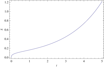
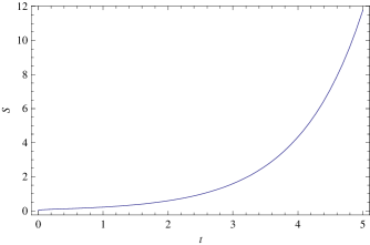
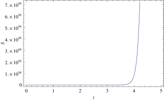
Figure 4: Evolution of scalar factor in the $\epsilon=+1$ case, with different values of $r_{c}=2,1,0.1$ for $\Sigma=0.001$. The figure shows that scale factor grows faster for small values of $r_{c}$, compaired to higher values.

$$\dot{H}+H^{2}\simeq-\mu^{2}(\rho+p)+\frac{1}{r_{c}^{2}}+\frac{2}{3}\mu^{2}\rho-2\frac{\Sigma^{2}}{S^{6}}>0,$$ (38)

and this gives,

$$p<-\frac{\rho}{3}+\frac{1}{\mu^{2}r_{c}^{2}}-\frac{2\Sigma^{2}}{\mu^{2}S^{6}}.$$ (39)

Similarly for the $\epsilon=-1$ case, expanding (32) and considering the next order, the Friedmann equation is,

$$H^{2}=\frac{\mu^{4}r_{c}^{2}}{9}\rho^{2}+\frac{\Sigma^{2}}{S^{6}}.$$ (40)

Notice that the relation between the Hubble radius and energy density is linear, a feature of brane sas ; lang , which is referred to as the fully 5D regime. The acceleration condition,

$$\dot{H}+H^{2}\simeq-\frac{\mu^{4}r_{c}^{2}}{3}\rho(\rho+p)+\frac{\mu^{4}r_{c}^{2}}{9}\rho^{2}-2\frac{\Sigma^{2}}{S^{6}}>0,$$ (41)

implies

$$p<-\frac{2\rho}{3}-\frac{6\Sigma^{2}}{S^{6}\mu^{4}r_{c}^{2}\rho}.$$ (42)

Therefore, one can see that the condition is modified compared to the standard cosmology and our results reduce to gumj in the absence of anisotropy.

Next we consider the inflationary phase driven by a scalar field, with energy density and pressure given by $\rho=\frac{1}{2}\dot{\phi}^{2}+V(\phi)$ and $p=\frac{1}{2}\dot{\phi}^{2}-V(\phi)$, respectively. The Klein-Gordon equation for a scalar field is ${\ddot{\phi}}+3H{\dot{\phi}}+V^{\prime}(\phi)=0$. Using Eq. (39) the slow-roll condition for inflation can be obtained for $\epsilon=1$ case as,

$$\dot{\phi}^{2}<V+\frac{3}{2\mu^{2}r_{c}^{2}}-\frac{3\Sigma^{2}}{S^{6}}.$$ (43)

It can be seen that the condition depends on the anisotropy and in the ordinary DGP conditon is recovered in absence of $\Sigma$ . Similarly for $\epsilon=-1$, using eqn (42) the slow roll condition is obtained as,

$$\dot{\phi}^{2}<-4V+2\sqrt{3V^{2}+\frac{18\Sigma^{2}}{S^{6}\mu^{4}r_{c}^{2}}}.$$ (44)

IV Conclusions

To summarize, we considered anisotropic effects in the DGP cosmological scenario and found a solution to the corresponding field equation. We obtained the Friedmann equations with the Bianchi-I brane and two branches of solutions in the DGP model are considered. The evolution of a scale factor in the case of the late universe is studied and an acceleration condition for inflation is derived.

It is observed that, for the $\epsilon=+1$ case, there exists a self-inflationary solution which leads to accelerated expansion in the late universe, even in the presence of anisotropy. The evolution of a scale factor is given in Fig. 1, which shows that the presence of shear does not stop the universe from entering a self-accelerated phase, but slows it down. The evolution scale factor in the anisotropic DGP model depends on the cross-overscale and the shear. It is noted that, when shear is unity($\Sigma=1$), the evolution of a scale factor coincides with the isotropic DGP model. Fig.2 shows dependence of a scale factor on the shear and the higher the value of $\Sigma$ the faster the universe enters into a self-accelerated phase. Fig.4 shows the behavior of a scale factor with typical values of a crossover scale $r_{c}$ and shows that the higher the $r_{c}$ the slower the acceleration. Hence, in the DGP model shear and $r_{c}$ behave oppositely to each other. The behavior $S$ for the $\epsilon=-1$ branch of the solution of the Friedmann equation is shown in Fig.3 and a scale factor grows faster for higher values of anisotropy. The scale factor grows as $S\propto t^{1/3}$ which implies slower expansion than the standard cosmology and is similar to expansion rate that of Randall-Sundrum case. The Friedmann equation in this case is similar to the RS Friedmann equation with quadratic energy density. The acceleration conditions and slow-roll conditions for inflation are obtained and they depend on the shear.

Finally, our results coincide with those of Deffayet def whenever $\Sigma$ is absent and reduce to the Bianchi-I of the general relativity under condition (30). Hence, the presence of initial anisotropy does not adversely affect the features of the DGP model. It is possible to have an anisotropic brane in the DGP model and still get a self-accelerating universe in the late time, as the anisotropic term appearing in (33) is not like energy density. Also, for a large value of $S$ ($S\rightarrow\infty$), the anisotropic term tends towards zero and we recover the isotropic case.

It can be noticed that in the present work, ghost like instabilities in the self-acclerated branch, as pointed out by ant , do not appear. This may be due to the fact that we are using special boundary conditions. So, it is interesting to study the self-accelerated branch with a ghost term, by solving the full brane-bulk system and considering more realistic boundary conditions, which is beyond the scope of the present paper.

References

- (1) P. Brax and C Bruck, Class. Quantum Grav 20 R201 (2003).
- (2) L. Rndall and R. Sundrum, Phys. Rev. Lett. 83, 3370(1999), 83 4690, (1999).
- (3) G.Dvali, M.Gabadadze and M.Porrati, PL B 485 , 208(2000).
- (4) Misner C W, ApJ 151, 431 (1968), Hu B L and Parker L, Phys. Rev.D 17, 933 (1978), Jacob K C, ApJ 153, 661 (1968), MacCallum M A H, , edited by Hawking S W and Israel W ( Cambridge University Press, 1979).
- (5) R Maartens, V Sahni and Tarun Deep Saini. Phys. Rev. D 63, 063509 (2001).
- (6) A.Campos and C. F. Sopuerta, Phys. Rev. D 63, 104012 (2001).
- (7) A. Toperensky, Class. Quantum Grav. 18, 2311 (2001).
- (8) B C. Paul, Phys. Rev. D 64, 124001 (2001).
- (9) G.Niz, A. Padilla and Hari.K. Kunduri, JCAP 0804,12 (2008).
- (10) A. Coley Phys. Rev. D 66, 023512 (2002) ,A .V. Frolov, PL B 514 ,213 (2001). M Santos, F. Vernizzi and P Ferriera, Phys. Rev. D 64, 063506 (2001), S. Hervik, Astrophys. Space Sci. 283, 673 (2003).
- (11) R. Gregory, N. Kaloper, R. C. Myers and A. Padilla, JHEP 0710, 069,(2007), A. Padilla J.Phys.A40, 6827-6834,(2007), C Charmousis, R Gregory, N. Kaloper and A. Padilla, JHEP 0610, 066,(2006), D. Gorbunov, K. Koyama and S. Sibiryakov, Phys.Rev.D 73, 044016,(2006),K. Koyama, Phys.Rev.D 72,123511,2005.
- (12) Rizwan ul Haq Ansari and P. K. Suresh, JCAP 09,21 (2007).
- (13) T. Shiromizu, K. Maeda and M. Sasaki, Phys. Rev. D 62, 024012 (2000).
- (14) S. Hawking and G. Ellis, The large scale structure of the Universe Cambrdge University Press, Cambridge (1973).
- (15) R. Maartens, Phys. Rev. D 62, 084023 (2000).
- (16) C. Deffayet Phys.Lett.B502:199-208 (2001).
- (17) B.Gumjudpai, Gen Rel and Grav 36, 747(2004).
- (18) P. Binetury, C. Deffayet and D. Langlois Nucl. Phys B 565 269 (2000).