Static and Impulsive Models of Solar Active Regions

Abstract

The physical modeling of active regions (ARs) and of the global coronal is receiving increasing interest lately. Recent attempts to model ARs using static equilibrium models were quite successful in reproducing AR images of hot soft X-ray (SXR) loops. They however failed to predict the bright EUV warm loops permeating ARs: the synthetic images were dominated by intense footpoint emission. We demonstrate that this failure is due to the very weak dependence of loop temperature on loop length which cannot simultaneously account for both hot and warm loops in the same AR. We then consider time-dependent AR models based on nanoflare heating. We demonstrate that such models can simultaneously reproduce EUV and SXR loops in ARs. Moreover, they predict radial intensity variations consistent with the localized core and extended emissions in SXR and EUV AR observations respectively. We finally show how the AR morphology can be used as a gauge of the properties (duration, energy, spatial dependence, repetition time) of the impulsive heating.

1 Introduction

Modeling ensembles of coronal loops in active regions or over the full Sun is a rapidly emerging new field in the study of the solar corona. Such studies attempt to reproduce generic properties of ARs and of the global corona such as space integrated intensities and overall morphology. This allows for the determination various properties of coronal heating such as its dependence on loop length and magnetic field thereby testing coronal heating mechanisms. Moreover such studies eliminate potential selection effects which may enter into studies of individual loops. Finally, AR and global coronal models pave the way for the construction of physics-based models of the EUV and SXR irradiance, an important contributor to Space Weather conditions.

The majority of the attempted AR and global coronal models were based on static equilibrium coronal loop models produced with steady heating (Schrijver et al. 2004; Mok et al. 2005; Warren $\&$ Winebarger 2006; Lundquist, Fisher $\&$ McTiernan 2007). They were quite successful at reproducing the general appearance of the corona in hot emissions ($>$ 3 MK) observed in the SXR by the Soft X-ray Telescope (SXT) on Yohkoh. However, synthetic EUV images from the static models did not show evidence of the warm loops seen in the real observations, but instead were dominated by intense footpoint (moss) emission. Steady heating that is highly concentrated near the coronal base can produce time dependent behavior called thermal non-equilibrium. This gives rise to transient EUV loops (Mok et al. 2008; Klimchuk, Karpen, & Patsourakos 2007), but whether their properties are fully consistent with observations has yet to be determined.

Most theories of coronal heating predict that energy is released impulsively on individual flux strands (Klimchuk 2006). This includes both AC (wave) and DC (reconnection-type) heating. Following this paradigm coronal loops are viewed as ensembles of unresolved, impulsively heated strands. A very promising idea first proposed by Parker (1988) is that the coronal field becomes tangled on small scales due to the random footpoint motions associated with turbulent photospheric convection. Current sheets develop at the interfaces between individual misaligned strands, and it has recently been shown that an explosive instability called the secondary instability occurs when the misalignment angle reaches a critical value (Dahlburg, Klimchuk $\&$ Antiochos 2005). This may be the physical nature of the nanoflares postulated by Parker. The heating function we have used in our simulations is appropriate to nanoflares that are initiated at a critical angle. We note that the upward Poynting flux associated with observed photospheric field strengths and observed photospheric velocities is consistent with coronal heating requirements (e.g. Abramenko, Pevtsov $\&$ Romano 2006), but the efficiency of field line tangling is only now being addressed quantitatively with high resolution magnetogram movies from Hinode. We also note that direct observations of the kinds of nanoflares we are discussing are scarce (Katsukawa $\&$ Tsuneta 2001). The small distinct brightenings that are sometimes called nanoflares are much different from the unresolved energy releases on long field lines that we consider here.

But why do static equilibrium models fail to reproduce the coronal emission patterns in the EUV? Can impulsive heating models do any better? And how can AR morphology be used to infer the properties of impulsive heating? With this paper we address these important questions.

2 AR Simulations

For the calculations reported in this paper we use the 0D hydrodynamic loop model we call enthalpy-based thermal evolution of loops (EBTEL), described in Klimchuk, Patsourakos $\&$ Cargill (2008). For a given temporal profile of the heating EBTEL calculates the temporal evolution of the spatially averaged temperature, density, and pressure along the loop. It also provides the Differential Emission Measure distribution (DEM(T)) for both the coronal and footpoint (i.e., transition region) sections of the loop. For steady heating, static equilibrium solutions are calculated. EBTEL is capable of relatively accurately mimicking complex 1D hydrodynamic simulations, with however much less demands in terms of CPU time, which makes it particularly useful for parametric investigations of multitudes of loops. We calculated hydrodynamic models for 26 loops with lengths in the range 50-150 Mm, typical of observed AR loops. For the construction of the AR images we assumed that the loops have semi-circular shapes and are nested the one on top of the other, forming an arcade which emulates the simplest form of AR topology.

2.1 Static Models

We first calculated a static equilibrium AR model. The steady volumetric heating $H$ supplied to a loop with length $L$ was :

$$H=H_{0}{(L/L_{0})}^{\alpha},$$ (1)

with $H_{0}$ the heating magnitude, $L_{0}$ the length of the shortest loop and $\alpha$ a scaling-law index which depends on the details of the specific coronal heating mechanism (e.g., Mandrini et al. 2000). We chose $L_{0}=50$ Mm, $H_{0}$=0.01   $\mathrm{erg\,{cm}^{-3}{s}^{-1}}$, and $\alpha=-2.8$. This particular $\alpha$ corresponds to heating associated with the tangling of the magnetic field by photospheric convection. A nanoflare occurs when the misalignment between adjacent flux strands reaches a critical angle. Similar $\alpha$ values were found to provide the best match between static models and AR and full Sun SXR images (Schrijver et al. 2002; Warren $\&$ Winebarger 2006; Lundquist, Fisher $\&$ McTiernan 2008). In concert with these studies, $H_{0}$ was chosen so that the temperature of the shortest and consequently hottest (according to Equation 1) loop of the arcade was $\approx$ 4 MK, consistent with the temperature of bright SXR loops in AR cores. The $DEM$ distributions for the coronal and footpoint sections of each simulated loop were folded with the temperature response functions of the 171 Å  and AlMg channels of TRACE and SXT respectively to determine the corresponding intensities. For the calculation of the intensities we assumed that simulated loops had a diameter of 3 Mm, consistent with typical widths of observed loops.

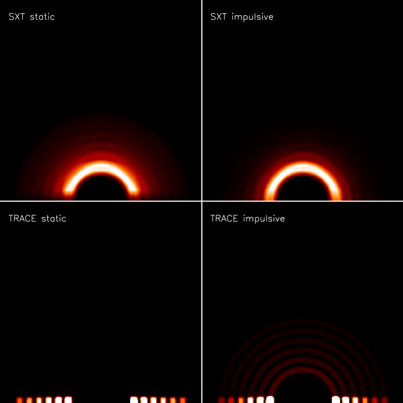
Figure 2: SXT and TRACE images of the simulated AR loop arcade for static equilibrium (left column) and impulsive heating (right column). The images for the impulsive heating correspond to a time-average over the corresponding simulations. It is assumed that the AR is observed face-on. The images are smoothed with boxcars consistent with the instrument resolution. The AR baseline has a length of $\approx$ 100 Mm. Intensity represented with color increasing from black to red to white. Each image is normalized individually.

In Figure 1 (left column) we plot the variation of intensity across the loop arcade while in Figure 2 (left column) we display the corresponding synthetic images. For building the images we assume that the AR is viewed face-on and for clarity reasons we display every fourth loop of our arcade. We applied convenient box-cars to the images to emulate the different spatial resolution of SXT ($\approx$ 5 arcsec) and TRACE ($\approx$ 1 arcsec). We assumed that the coronal emission is distributed uniformly along the loop. This is reasonable because our loops are shorter than a gravitational scale height, so there will be minimal gravitational stratification. Furthermore, the coronal temperature varies by only about $50\%$ along most of the length of equilibrium loops (Klimchuk et al. 2008). Temperature and density of course vary dramatically in the transition region, but the thickness of transition region is generally unresolvable, so we spread the emission over 2 Mm for convenience and clarity. The magnitude of the integrated transition region emission is correct.

From Figure 1 we note that the SXT emission is considerably weaker at the footpoints than in the corona. This is because the footpoint temperatures are generally below 2 MK, where SXT has greatly reduced sensitivity. Furthermore, from Figure 2 the synthetic TRACE image is completely dominated by the footoints. There is little evidence of EUV loops, which is at odds with the multitudes of EUV loops seen in the majority of observed ARs. Our results are broadly consistent with previous studies employing static heating.

Why is it that static equilibrium models fail to predict bright EUV loops together with bright SXR loops? This ”pathology” is related to the fact that under static equilibrium conditions the loop temperature has a very weak dependence on the loop length. For instance, the Rosner et al. (1978) scaling law predicts that the apex temperature is related to the heating rate and length according to $T_{a}\propto{H}^{2/7}L^{4/7}$. Therefore, for the employed value $\alpha=-2.8$ we have from Equation 1 that $T_{a}\propto L^{-0.22}$. This means that the temperature is reduced by a factor of only $3^{-0.22}=0.8$ in going from the shortest loop (4 MK) to the longest loop (3.1 MK) in the arcade. As shown Figure 3, our simulations closely follow the above scaling law. Therefore, none of the loops has 1-2 MK plasma in the coronal section, which is necessary to produce significant EUV emission. All of this plasma resides at the footpoints, which is where the strong TRACE emission originates. Obviously, we could decrease $H_{0}$ to produce strong TRACE emission in the corona, but then the SXT emission would be dramatically reduced. The only way to have both bright TRACE loops and bright SXT loops in the same arcade is for the heating rate to have a much stronger dependence on loop length. Our example arcade requires $\alpha\simeq-6$. We are not aware of any coronal heating mechanism with such an extreme dependence on $L$ (e.g. Mandrini et al. (2001)).

2.2 Impulsive Models

We then considered models with impulsive heating, using the same loop arcade of the previous section. We started with static equilibria having an average coronal temperature near 0.5 MK. We heated the loops with a triangular pulse lasting 50 s and let the loops cool for 8500 s, by which time the temperature had cooled below 1 MK. The amplitude of the heat pulses varied from loop to loop according to Equation 1, with $\alpha=-2.8$, as before, and $H_{0}=2.5\,\mathrm{erg\,{cm}^{-3}\,{s}^{-1}}$. This produced an average $DEM$ for the arcade that peaks near 2.0 MK, similar to that of observed active regions (e.g., Brosius et al. 1996). Each loop reaches a maximum temperature exceeding 30 MK (Figure 3), but this happens very early in the heating event, when the density is very low. The $DEM$-weighted mean temperature $T_{DEM}$ is only 1-2 MK.

We determined temporally averaged TRACE and SXT intensities for each loop simulation. Time averaging over the duration of a loop simulation is equivalent to taking a snapshot of a loop containing a large number of impulsively heated unresolved strands at different stages of heating and cooling. As before, we produced synthetic images of the arcade by assuming that the time-averaged intensities are uniform along each the loop. Our 1D hydro simulations indicate that this is a reasonable approximation (e.g., Klimchuk et al. 2006). The right columns of Figures 1 and 2 show the intensity variation across the arcade and the synthetic image, respectively.

We note in Figure 1 that the TRACE emission from the footpoints is a factor of $\approx$ 3-100 smaller for impulsive heating than for static heating, wheres the coronal emission is about the same in the two cases. The brightness contrast between the footpoints and corona is therefore significantly reduced for impulsive heating. This leads to a TRACE image in which both the coronal and footpoint emissions can be readily discerned (Figure 2 right panel). This is not true for the static model (left panel), where the coronal emission is overwhelmed by the footpoint emission. The footpoint to corona intensity ratios $I_{foot}/I_{corona}$ are of order 10 in the impulsive model and 1000 in the static model. Observed values are in the range $\approx$ 2-20. The smaller observed ratios could be due to spicular absorption of the footpoint emission (e.g., Daw, Deluca $\&$ Golub 1995; De Pontieu et al. 1999). Using the analytical expressions of Anzer $\&$ Heinzel (2005) for absorption at TRACE wavelengths and typical physical parameters of spicules given in Table-1 of Tsiropoula $\&$ Schmieder (1993) we found that attenuation factors of the 171 TRACE emission of about 10 can be achieved. As a matter of fact a recent SUMER/EIS study of moss intensities formed above and below the head of the hydrogen Lyman continuum at 912 Å  demonstrated that indeed sizeble absorption occurs over moss regions (De Pontieu et al. 2008). Future AR models would probably need to incorporate absorption effects. Warren and Winebarger (2007) modeled an observed AR using 1D simulations and also found that impulsive heating increases the visibility of EUV loops compared to static equilibrium.

It can also be seen in Figure 1 that brightness of the corona in TRACE relative to SXT is roughly two orders of magnitude larger in the impulsive model than in the static model. This suggest that bright TRACE loops are much more likely to be seen together with bright SXT loops in the same active region if the heating is impulsive.

The increased TRACE-to-SXT coronal intensity ratio and the reduced footpoint-to-corona TRACE contrast can both be understood as follows. In static equilibrium, the optimum temperature for a particular waveband occurs either in the corona or at the footpoints, but not at both locations. For apex temperatures $>$ 2 MK, the coronal plasma is too hot to emit appreciable TRACE emission, and only the footpoints are bright. This is the case for all of the loops in the static arcade. Impulsively heated loops are fundamentally different in that they experience a wide range of coronal and footpoint temperatures over the course of their evolution. When an impulsively heated loop starts to cool, TRACE emission occurs first at the footpoints and then over the full length of the loop when the coronal temperature drops below 2 MK. A bundle of impulsively heated strands will therefore have significant TRACE emission both in the corona and at the footpoints.

A final interesting property revealed in Figure 1 is the distribution of coronal emission across the arcade. SXT intensities decrease rapidly with loop length, especially in the impulsive model, while TRACE intensities decrease much more slowly. As a consequence, the SXT emission is concentrated in the core of the arcade, and the TRACE emission is much more extended (Figure 2). This agrees well with AR observations. The strong decrease in the SXR emission with increasing $L$ is because $T_{DEM}$, the dominant temperature of the plasma, drops below 2 MK for the longer loops (Figure 3). The sensitivity of SXT is a rapidly decreasing function of temperature in this range. On the other hand, the $T_{DEM}$ values are in the range where TRACE has good sensitivity, so the TRACE intensity gradient across the arcade is more shallow.

We then examined how the AR morphology depends on the properties of the impulsive heating. We first considered the effect of varying the index $\alpha$ of Equation 1 by taking the following values: -4, -3, -2, -1. All other aspects of the simulation were the same as for the $\alpha=-2.8$ base simulation discussed above. The resulting intensity variations across the loop arcade for TRACE and SXT are given in Figure 4. Not surprisingly, we found that a stronger dependence of impulsive heating on $L$ (i.e. a more negative $\alpha$) produces a steeper intensity drop-off across the arcade. Note that that if we were to observe our arcade off-limb, the model with $\alpha$=-1 would yield an intensity scale-height consistent with off-limb observations of the unresolved EUV corona (Cirtain et al. 2005).

The impact of the time-interval between successive nanoflares, ${\Delta\tau}_{nano}$, assuming the dependence ${\Delta\tau}_{nano}={\Delta\tau}_{0}{(L/L_{0})}^{\gamma}$ was then examined. We consider two cases: (1) $\gamma=-2$ and ${\Delta\tau}_{0}=8500$ s; (2) $\gamma=2$ and ${\Delta\tau}_{0}=250$ s. For each loop we considered 3 consecutive nanoflares separated by ${\Delta\tau}_{nano}$. The nanoflare heating rate and duration were the same as in the base simulation which implies the same averaged energy per nanoflare. When ${\Delta\tau}_{nano}$ decreases with $L$ (case 1) the resulting images (left column of Figure 5) are characterized by TRACE emission concentrated around the AR core while the SXT emission is extended. This is because the longest loops in the arcade have ${\Delta\tau}_{nano}$ of about 850 s which is not sufficient to let them cool down to TRACE temperatures. On the other hand, when ${\Delta\tau}_{nano}$ increases with $L$ (case 2), the resulting AR images are characterized by bright core emission in SXT and lack of TRACE loops (right column of Figure 5). This is because shorter loops do not have the time to cool down to TRACE temperatures and they remain in quasi-steady state conditions in SXT temperatures, as also shown in Section 2.1. This model can explain observations of an AR with SXT loops but no TRACE loops (Antiochos et al. 2003).

We then investigated the effect of the magnitude of the nanoflare energy on the SXT and TRACE coronal and moss intensities respectively. These intensities are particularly useful when studying the cores of active regions and can constrain the properties of the heating (e.g. Winebarger, Warren $\&$ Falconer 2007). On top of the base model described in the first paragraph of this section, we considered 3 additional AR models employing nanoflare heating magnitudes 2,6 and 10 times the one used in the base simulation (see also Equation 1). All other aspects of these simulations were the same as for the base simulation. The variation of the temporally averaged intensities across the loop arcade for the 4 models is shown in Figure 6. What can be seen in this Figure is that increasing nanoflare energy leads to higher SXT coronal to TRACE moss intensity ratio $I_{SXR}/I_{EUV-moss}$. For instance, for the inner loops in the modeled AR (i.e. its core) $I_{SXR}/I_{EUV-moss}$ increases from $\approx$ 1.3 to 4.4 with a 10-fold increase in the nanoflare energy. This means that $I_{SXR}/I_{EUV-moss}$ tracks in a rather sensitive way the nanoflare energy and can be used as its diagnostic. Is it worth mentioning that the determined trend goes in the direction of decreasing the discrepancy with observations that can cause problems with static models. Possibly the spicular absorption discussed in the previous paragraphs could bring $I_{SXR}/I_{EUV-moss}$ even to a better agreement with the observations

We finally found that the nanoflare duration does not alter the AR morphology for both SXT and TRACE. This comes to no surprise given both instruments are mostly sensitive to the late cooling of the impulsively heated loops, when any differences in the loop response for different nanoflare durations, had been long ago smeared out (e.g. Patsourakos $\&$ Klimchuk 2005).

3 Conclusion

With this work we considered static and impulsive heating models of active region arcades. In concert with previous investigations, we found that static models cannot simultaneously reproduce bright EUV and SXR loops withing the same AR. We showed that this is due to the shallow dependence of loop temperature on loop length implied by all reasonable coronal heating scenarios. We found that impulsive heating models agree much better with observations than do static models. In particular, impulsive heating produces (1) a reduced brightness contrast between the corona and footpoints in TRACE observations, (2) an increased TRACE-to-SXT coronal intensity ratio, and (3) enhanced SXT emission in the core of the active region and extended TRACE emission. We finally showed that the AR morphology depends rather sensitively on the properties of impulsive heating, like its spatial dependence and the time interval between successive nanoflares, and can therefore be used to determine the properties of the heating. Our study paves the way for detailed comparisons between multi-temperature observations of ARs and models based on impulsive heating and detailed reconstructions of the coronal magnetic field from extrapolations.

Research supported by NASA and ONR. We acknowledge useful discussions with the members of the ISSI team ”The role of Spectroscopic and Imaging Data in Understanding Coronal Heating” (team Parenti).

Figure 1: Variation of the intensity across the loop arcade for static equilibrium (left column) and for impulsive heating (right column) for SXT and TRACE. We plot the intensities for both the coronal (solid line) and transition region section (dashed line) of the loops. For impulsive heating the time-averaged intensities are plotted. Intensities are in units of DN/pix/s.

Figure 3: Variation of the temperature across the loop arcade. Static equilibrium model (solid line) and fit $\propto$ $L^{-0.22}$ (dash-triple dot). Impulsively heated model: maximum temperature divided by 10 (dashed line); $DEM$-weighted mean temperature (dashed-dotted line).

Figure 4: Variation of the normalized coronal intensity across the loop arcade for different values of the power-law index $\alpha$, determining how the nanoflare energy is distributed across loops with different $L$, for TRACE (left panel) and SXT (right panel).

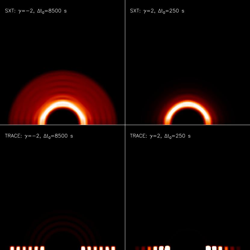
Figure 5: Investigating the effect of the time-interval ${\Delta\tau}_{nano}$ between successive nanoflares. Synthetic TRACE and SXT images for ${\Delta\tau}_{nano}$ which decreases (increases) with loop length left (right) column. The AR baseline has a length of $\approx$ 100 Mm. Intensity represented with color increasing from black to red to white. Each image is normalized individually.

Figure 6: Variation of the coronal and footpoint intensity across the loop arcade for SXT (left panel) and TRACE (right panel) respectively for impulsively heated AR models with different nanoflare energies. The nanoflare magnitude for each AR model are 4 (dots), 6 (long dashes), 10 (dash-dot) times that of the base model (solid). The time-averaged intensities are plotted. Intensities are in units of DN/pix/s.

References

- (1) Abramenko, V. I., Pevtsov, A. A., Romano, P. 2006, ApJ, 646, L81
- (2) Anzer, U. Heinzel, P. ApJ, 2005, 622, 714
- (3) Brosius, J. W., Davila, J. M., Thomas, R. J. Monsignori-Fossi, B. C. 1996, ApJS, 106, 143
- (4) Cirtain, J., Martens, P. C. H., Acton, L. W. Weber, M. 2006, Sol Phys, 235, 295
- (5) Dahlburg, R. B., Klimchuk, J. A., Antiochos, S. K. 2005, ApJ, 622, 1191
- (6) Daw, A., Deluca, E. E. Golub, L. 1005, ApJ, 453, 929
- (7) De Pontieu, B., Berger, T. E., Schrijver, C. J., Title, A. M. 1999, Sol. Phys., 190, 419
- (8) De Pontieu, B. et al. 2008, ApJ, in preparation
- (9) Katsukawa, Y., Tsuneta, S. 2001, ApJ, 557, 34
- (10) Klimchuk, J. A. 2006, Solar Phys., 234, 41
- (11) Klimchuk, J. A., Karpen, J. T., Patsourakos, S. 2007, Eos Trans. AGU, 88(52), Fall Meet. Suppl., Abstract SH51C-05
- (12) Klimchuk, J. A., Lopez Fuentes, M. C., DeVore, C. R. 2006, in Proceedings of SOHO-17: Ten Years of SOHO and Beyond (ESA SP-617), ed. H. Lacoste (Noordwijk: ESA)
- (13) Klimchuk, J. A., Patsourakos, S. Cargill, P. J. 2008, ApJ, in press
- (14) Klimchuk, J. A., Cargill, P. J. 2001, ApJ, 553, 440
- (15) Lundquist, L. L., Fisher, G. H., McTiernan, J. M., 2008, ApJ, in press
- (16) Mandrini, C. H., Dèmoulin, P., Klimchuk, J. A. 2000, ApJ, 530, 999
- (17) Mok, Y., Mikic, Z., Lionello, R. Linker, J. A. 2005, ApJ, 621, 1098
- (18) Mok, Y., Mikic, Z., Lionello, R. Linker, J. A. 2008, ApJ, 679, L161
- (19) Parker, E. N. 1988, ApJ, 330, 474
- (20) Patsourakos, S., Klimchuk, J. A. 2005, ApJ, 628, 1023
- (21) Porter, L. J., & Klimchuk, J. A. 1995, ApJ, 454, 499
- (22) Rosner, R., Tucker, W. H., Vaiana, G. S. 1978, ApJ, 220, 643
- (23) Schrijver, C. J., Sandman, A. W., Aschwanden, M. J., DeRosa, M. L. 2004, ApJ, 615, 512
- (24) Tsiropoula, G. Schmieder, B. 1997, A, 324, 1183
- (25) Warren, H. P. Winebarger, A. R. 2006, ApJ, 645, 711
- (26) Warren, H. P. Winebarger, A. R. 2007, ApJ, 666, 1245
- (27) Winebarger, A. R., Warren, H. P. Mariska J. T. 2003, ApJ, 587, 439
- (28) Winebarger, A. R., Warren, H. P., Falconer, D. A. 2008, ApJ, 676, 672