Ionization front-driven turbulence in the clumpy interstellar medium

Abstract

We present 3D radiation-gasdynamical simulations of an ionization front running into a dense clump. In our setup, a B0 star irradiates an overdensity which is at a distance of $10\,\mathrm{pc}$ and modelled as a supercritical $100\,M_{\astrosun}$ Bonnor-Ebert sphere. The radiation from the star heats up the gas and creates a shock front that expands into the interstellar medium. The shock compresses the clump material while the ionizing radiation heats it up. The outcome of this “cloud-crushing” process is a fully turbulent gas in the wake of the clump. In the end, the clump entirely dissolves. We propose that this mechanism is very efficient in creating short-living supersonic turbulence in the vicinity of massive stars.

I Introduction

Massive stars strongly influence the environment in which they have formed by stellar winds, ionizing radiation and supernova explosions. An ionization front which expands into the ambient interstellar medium (ISM) and hits a dense clump may compress it so heavily that gravitational collapse might be triggered. On the other hand, ionization heats up the material and can photoevaporate the clump. The remaining material of this competition may form low-mass stars hest05 or brown dwarfs whit04 .

The interaction of a shock with a dense clump is called “cloud-crushing”. The cloud-crushing scenario has been studied numerically both for supernova shocks and ionization fronts. The first extensive studies of the fate of the shocked cloud already showed that strong vortex rings can be produced klein94 . The mixing properties of the cloud depend sensitively on the initial density distribution naka06 . Furthermore, simulations of dense clumps exposed to an ionizing flux but without strong shocks show the generation of kinetic energy kessel03 and fragmentation of the clump esquivel07 . Radiation-gasdynamical simulations have also been used to match observations in H II regions, especially the Eagle Nebula williams01 ; miao06 .

Although ionizing radiation injects a significant amount of energy into the ISM, it does not seem to be an important driving mechanism of interstellar turbulence on a global scale maclow04 . However, the cloud-crushing process generates a considerable amount of turbulence locally in the wake of the cloud. We find that the motion of the cloud material is mostly supersonic while the ambient gas behind the front moves only subsonically. The continuous heating limits the lifetime of the dense material, but the supersonic motions are maintained until the cloud disperses. This is contrary to the situation in jet-clump interactions, where the situation is less clear with some studies showing mostly subsonic motions baner07 while others claim supersonic velocity fields li07 .

II Numerical methods

We perform 3D radiation-gasdynamical adaptive mesh simulations with the FLASH code fryxell00 , which is based on the PARAMESH library macneice00 . In addition to the refinement with respect to shocks we also make sure that we resolve the Jeans length with a sufficient number of cells to avoid artificial fragmentation truelove97 ; baner04 . The Jeans length is the critical scale for self-gravitating objects, and a dynamical increase of resolution would indicate a runaway collapse. However, the run discussed in this paper show collapse only temporarily.

Additionally to the standard hydrodynamics and self-gravity, we include the ionization feedback from a massive star. The radiation feedback is included via a raytracing approach rijk06 . There are no radiation pressure terms in the Euler equations; in this module coupling between hydrodynamics and radiation takes place only through thermodynamics. We solve a rate equation for the ionization fraction including collisional ionization and photoionization as well as radiative recombination. The energy equation contains a photoionization heating rate; the equation of state is isothermal.

III Setup

The computational domain has dimensions $(6.0\times 2.4\times 2.4)\cdot 10^{19}\,\mathrm{cm}$ with an effective resolution of $512\times 256\times 256$ cells. We place a self-gravitating supercritical gas sphere with Bonnor-Ebert density profile bonnor56 ; ebert55 , with mass $M=100\,M_{\astrosun}$ in the centre of the domain. It slowly rotates with an angular velocity of $\Omega=7.83\cdot 10^{-15}\,\mathrm{rad}/\mathrm{s}$ around the $z$-axis corresponding to a ratio of rotational to gravitational energy of $\beta=0.02$. Additionally to the rotational velocity, a turbulent velocity field with a magnitude of at most 50% of the sound speed is added. The temperature of the Bonnor-Ebert sphere is $T=20\,\mathrm{K}$, while the ambient gas has $T=90\,\mathrm{K}$.

The ionizing source is located at the left hand side of the computational domain at $(0.0,1.2,1.2)\cdot 10^{19}\,\mathrm{cm}$. It has a temperature of $T_{\mathrm{s}}=29,200\,\mathrm{K}$ and a luminosity of $L_{\mathrm{s}}=24,000\,L_{\astrosun}$, representing a B0 star. The radiation heats the interstellar gas to $T\approx 6\cdot 10^{4}\,\mathrm{K}$.

IV Results

When the simulation starts, the gas next to the source becomes ionized and heated. An ionization front accompanied by a shock expands into the ISM. When the shock hits the clump, the clump material is swept away and thereby compressed heavily. The shock leaves behind a fully turbulent gas. The hot ionized gas is being mixed with the cold clump material while the radiation heats it up continuously. After the shock front passes the clump, the former clump disperses completely.

The time sequence of this process is as following. The shock touches the outer edge of the clump at $t=0.40\,\mathrm{Myr}$. At $t=0.53\,\mathrm{Myr}$, it reaches the clump centre at $x=3\cdot 10^{19}\,\mathrm{cm}$, and at $t=0.76\,\mathrm{Myr}$, the front has totally enclosed the clump. Of course, the dense material delays the shock, so that the wings of the front can propagate faster. They enter the shadow zone and meet in the middle at $t=0.77\,\mathrm{Myr}$. The clash of these wings is an important driving mechanism of the turbulence seen in these simulations. It builds up an extended turbulent wake while the ionization front propagates further into the ISM. At $t=1.09\,\mathrm{Myr}$, the shock reaches the boundary of the computational domain at $x=6\cdot 10^{19}\,\mathrm{cm}$. The simulation stops at $t=1.49\,\mathrm{Myr}$ when the cloud has dissolved. Some of the stages of this time evolution are depicted in figure 1.

V Discussion

V.1 Energy balance

We start our analysis with a brief look at the energy balance in the flow (see figure 2). The plot shows the total energy $E$, internal energy $E_{\mathrm{int}}$ and kinetic energy $E_{\mathrm{kin}}$ in $\mathrm{erg}$ as a function of time $t$. The B star provides energy to the system by ionising material. This contribution is predominantly transferred into internal energy by the photoionization heating, only a small fraction is converted into kinetic energy. For example, at $t=0.5\,\mathrm{Myr}$, the ratio of internal over kinetic energy is $E_{\mathrm{int}}/E_{\mathrm{kin}}\approx 57$.

Since the luminosity of the star is constant in time, the energy transferred from the star to the gas in the computational domain grows linearly. This explains qualitatively the form of $E(t)$ in figure 2. A quantitative analysis is difficult however, since geometric effects have to be taken into account appropriately. One would have to account for the fact that the star emits its radiation isotropically, while it is not at the centre of a spherically symmetric computational domain, but on one face of a Cartesian box.

V.2 Mach numbers

The simulation shows that the cloud-crushing flow is largely dominated by supersonic motion. This is because the cloud material is cold, so that the sound speed is much lower than in the hot gas behind the ionization front, where a wind with $\mathcal{M}\approx 0.2$–$0.4$ is observed. The cause of the wind is that the photoionization heating is stronger close the source, which leads to a pressure gradient and a corresponding flow. Since the wind prevails in the largest part of the domain, namely the hot postshock gas, the mean Mach number $\mathcal{M}_{\mathrm{mean}}$ is always below unity, while the maximum Mach number $\mathcal{M}_{\mathrm{max}}$, which is reached at crushing, can be greater than $6$.

Figure 3 depicts $\mathcal{M}_{\mathrm{max}}$ and $\mathcal{M}_{\mathrm{mean}}$ as a function of time. The maximum Mach number traces the shock ahead of the ionization front. Within a time of $0.15\,\mathrm{Myr}$, the shock accelerates up to a constant velocity of $\mathcal{M}=4$. For a short time of another $0.15\mathrm{Myr}$ the velocity seems to saturate, but the continuous photoionization heating accelerates the shock again up to $\mathcal{M}=6.5$. At this point, when $\mathcal{M}_{\mathrm{max}}$ is maximal, the shock collides with the dense clump. As it hits the high-density gas, the shock front moves more slowly. The gas decelerates, so that $\mathcal{M}_{\mathrm{max}}$ decreases again. However, the wings of the shock that were not affected by the clump can enter the shadow zone, which leads to a peak in $\mathcal{M}_{\mathrm{max}}$ after $0.7\,\mathrm{Myr}$. Then these wings collide, which stops the motion in $y$-direction, so that the Mach number decreases further. But the collision of the wings also leads to an acceleration in positive $x$-direction, which can be seen in a series of peaks from $0.8\,\mathrm{Myr}$ to $1.1\,\mathrm{Myr}$. After $1.1\,\mathrm{Myr}$, the shock leaves the computational domain, resulting in a sharp drop in $\mathcal{M}_{\mathrm{max}}$. This demonstrates that the highest Mach numbers are only reached in the shock front itself, not in the shock-generated turbulence behind the front. The motion in the turbulent wake is mostly supersonic with $\mathcal{M}$ below $3$. The mean Mach number grows continuously until the shock leaves the domain, whereafter $\mathcal{M}_{\mathrm{mean}}$ declines slowly. The heating of the gas does not change $\mathcal{M}_{\mathrm{mean}}$.

The different stages of the simulation can also be recognized in the probability density functions (PDFs) of the Mach number $\mathcal{M}$. Figure 4 shows mass-weighted PDFs at the moment of cloud-crushing ($t=0.49\,\mathrm{Myr}$) and after the shock has left the domain ($t=1.16\,\mathrm{Myr}$ to $t=1.45\,\mathrm{Myr}$). At the crushing time, the high $\mathcal{M}$ above $2$ all belong to the shock. The shock then excites supersonic turbulence in the wake, but away from the shock $\mathcal{M}$ above $3$ is very rare. While most of the dense gas is supersonic, most of the domain is dominated by low Mach number flows, both at crushing time and afterwards.

The PDFs of the total Mach number $\mathcal{M}$ should be compared with the Mach number given only by the turbulent velocity fluctuations, $v_{\mathrm{turb}}=\sqrt{v_{y}^{2}+v_{z}^{2}}$, which is $v_{\mathrm{turb}}/c_{\mathrm{s}}$, where $c_{\mathrm{s}}$ is the local speed of sound. These plots are shown in figure 5. Since the bulk motion in $x$-direction is no longer taken into account, the Mach numbers are significantly lower. At the moment of cloud-crushing, the turbulent Mach number is only slightly supersonic, while it is totally subsonic afterwards. Hence, the bulk motion of the shock (and also the transport of momentum by the wind) is important to reach the high Mach numbers observed above.

We are also interested in the fraction of mass which moves supersonically. In figure 6 we plot the ratio of the mass of supersonic gas $M_{\mathrm{sup}}$ and the total gas mass in the computational domain $M_{\mathrm{tot}}$. Despite of the complicated mixing processes, $M_{\mathrm{sup}}/M_{\mathrm{tot}}$ grows roughly linearly until the shock leaves the domain. It is surprising that a significant part of the gas moves supersonically, altough most of the energy input is converted into internal energy (see figure 2). When the shock front leaves the domain, more than $60\%$ of the gas in our domain is in supersonic motion.

V.3 Clump structure after crushing

In figure 7, we enlarge a part of figure 1 belonging to the snapshot at $t=1.27\,\mathrm{Myr}$ and show additionally to the mass density also the temperature and the velocity components $v_{x}$ and $v_{y}$. The remains of the dense core have a temperature around $T\approx 300\,\mathrm{K}$, while the ambient ionized medium is at $T\approx 3.5\cdot 10^{4}\,\mathrm{K}$. The high temperatures in the environment give rise to the “rocket effect”, which accelerates the gas in positive $x$-direction oort55 . This is because the cold gas at the surface of the clump facing the star becomes heated. Thus, it expands into the postshock medium, carrying momentum with it, and consequently the clump accelerates.

The cloud-crushing leads to vortical structures in the wake as can be seen from the lower plots in figure 7. The two largest structures around $x\approx 4.2\cdot 10^{19}\,\mathrm{cm}$ and $y\approx 0.7\cdot 10^{19}\,\mathrm{cm}$ or $y\approx 1.7\cdot 10^{19}\,\mathrm{cm}$, respectively, even have slightly negative $v_{x}$ and so does a region around the tip of the former core at $x=3.3\cdot 10^{19}\,\mathrm{cm}$ and $y=1.2\cdot 10^{19}\,\mathrm{cm}$. Averaged over the whole volume, however, the wind, wich moves with $v_{x}\approx 1.5\cdot 10^{6}\,\mathrm{cm}/\mathrm{s}$, causes a bulk motion of the gas in positive $x$-direction. In order to measure the turbulent components of the velocity field, it is better to focus on the transversal directions. The peak amplitude of the velocity component in $y$-direction, for example, is about half of the maximum velocity in $x$-direction. The large vortical structures discussed above have total velocities around $10^{6}\,\mathrm{cm}/\mathrm{s}$. The upper vortex rotates clockwise, while the lower vortex rotates counter-clockwise.

V.4 Line-of-sight velocity profiles

A connection to observations of molecular clouds can be made by looking at velocity profiles along a certain line-of-sight ossen02 . Examplary, we show in figure 8 a profile for $v_{y}$ of the dense core after crushing at time $t=1.27\,\mathrm{Myr}$ (compare also figure 7). The width of the beam is $3.0\cdot 10^{19}\,\mathrm{cm}\leq x\leq 4.0\cdot 10^{19}\,\mathrm{cm}$ and $0.7\cdot 10^{19}\,\mathrm{cm}\leq z\leq 1.7\cdot 10^{19}\,\mathrm{cm}$, while $y$ ranges over the whole box width. Note that the profile is a mass-weighted histogram, not a normalized PDF. We do the same calculation again, but this time only considering gas that has $T\leq 10^{3}\,\mathrm{K}$ (low $T$ case) or $T\geq 10^{4}\,\mathrm{K}$ (high $T$ case). From the figure we see that the high velocity tails are exclusively related to the high temperature gas. The peak at low velocities comes mainly from both the low temperature medium as well as a warm envelope with temperatures between the cuts $10^{3}\,\mathrm{K}\leq T\leq 10^{4}\,\mathrm{K}$. Additionally to the histograms, we have fitted Gaussians to the low and high $T$ data. Their variance gives a measure for the turbulent velocity and can be related to the width of spectral lines that are being oberserved.

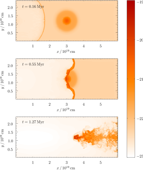
Figure 1: The main stages of the simulation are shown as 2D cuts of the logarithmic mass density $\log(\rho\,/\,\mathrm{g}\,\mathrm{cm}^{-3})$ in the midplane. The different snapshots are taken at times $t=0.16\,\mathrm{Myr}$, $t=0.55\,\mathrm{Myr}$ and $t=1.27\,\mathrm{Myr}$, respectively. The turbulent wake behind the former clump at the last stage is clearly visible.

Figure 2: The total energy $E$, internal energy $E_{\mathrm{int}}$ and kinetic energy $E_{\mathrm{kin}}$ are shown as function of time $t$. The major contribution to $E$ comes evidently from $E_{\mathrm{int}}$, while $E_{\mathrm{kin}}$ is between one and two orders of magnitude smaller. The point in time where the shock, which carries most of the kinetic energy, leaves the computational domain can be distinguished easily.

Figure 3: The average and maximum Mach numbers in the flow provide information on the dominance of shocks in the flow. To compare these two numbers, the mean Mach number $\mathcal{M}_{\mathrm{mean}}$ is displayed amplified by a factor of $5$. The peaks in $\mathcal{M}_{\mathrm{max}}$ can be associated with events in the cloud-crushing scenario.

Figure 4: The mass-weighted PDFs of the Mach number $\mathcal{M}$ between times $t=0.49\,\mathrm{Myr}$ and $t=1.45\,\mathrm{Myr}$. The shock front shows up as a peak in the regime of high Mach numbers for the first point in time. At $t=1.16\,\mathrm{Myr}$, the shock has left the computational domain, and the turbulence with its supersonic Mach numbers decays.

Figure 5: The mass-weighted PDFs of the “turbulent Mach number” $v_{\mathrm{turb}}/c_{\mathrm{s}}$ with $v_{\mathrm{turb}}=\sqrt{v_{y}^{2}+v_{z}^{2}}$ for the same points in time as in figure 4. At cloud-crushing, the turbulent field $v_{\mathrm{turb}}$ is slightly supersonic, while the flow in the wake is only subsonic. This shows that the bulk motion contributes significantly to the high total Mach numbers.

Figure 6: The fraction of gas in supersonic motion $M_{\mathrm{sup}}/M_{\mathrm{tot}}$ as a function of time $t$. Although most of the energy input goes into internal energy, more than half of the gas moves supersonically when the shock leaves the domain.

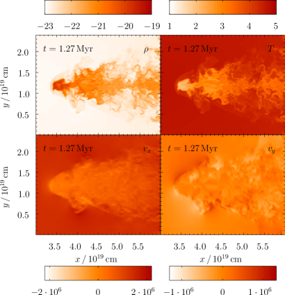
Figure 7: The midplane cuts at $t=1.27\,\mathrm{Myr}$ of the density $\log(\rho\,/\,\mathrm{g}\,\mathrm{cm}^{-3})$, the temperature $\log(T\,/\,\mathrm{K})$, the velocity in $x$-direction $v_{x}\,/\,\mathrm{cm}\,\mathrm{s}^{-1}$ and the velocity in $y$-direction $v_{y}\,/\,\mathrm{cm}\,\mathrm{s}^{-1}$ are compared with each other. The remains of the dense clump are still cold, while the material in the wake is already heating up. While $v_{y}$ is a measure for the turbulent velocity fluctuations, $v_{x}$ shows the bulk motion of the gas.

Figure 8: Line-of-sight mass-weighted histograms for $v_{y}$ around the dense core after cloud-crushing at time $t=1.27\,\mathrm{Myr}$ (in arbitrary units). The figure shows both the total data and the low temperature $T\leq 10^{3}\,\mathrm{K}$ and high temperature $T\geq 10^{4}\,\mathrm{K}$ cuts. Clearly, the high velocity contributions stem from the high $T$ gas, whereas the peak around zero relates mainly to the low $T$ gas and a warm envelope with $T$ between the two cuts. Also shown are Gaussian fits to the low and high $T$ cuts that give insight into the strength of the turbulent velocity fluctuations and can be compared with observed spectral line widths.

VI Conclusion

We have seen that cloud-crushing by ionization fronts can lead to short-living supersonic turbulence. Altough only a minute fraction of the energy input is converted into kinetic energy, up to $60\%$ of the affected gas is supersonic. While it is mainly the cold gas that is highly supersonic, it is the hot gas that moves the fastest. The bulk motion of the shock is an important contribution to the supersonic flow, since the transversal fluctuations are at best slightly supersonic.

References

References

- (1) Hester J J and Desch S J 2005 Understanding Our Origins: Star Formation in H II Region Environments Chondrites and the Protoplanetary Disk, Astron. Soc. Pac. Conf. Ser. 341 Edited by Krot A N, Scott E R D and Reipurth B (San Francisco: Astronomical Society of the Pacific) 107–130
- (2) Whitworth A P and Zinnecker H 2004 The formation of free-floating brown dwarves and planetary-mass objects by photo-erosion of prestellar cores Astr. Astrophys. 427 299–306
- (3) Klein R I, McKee C F and Colella P 1994 On the Hydrodynamic Interaction of Shock Waves with Interstellar Clouds. I. Nonradiative Shocks in Small Clouds Astrophys. J. 420 213–36
- (4) Nakamura F, McKee C F, Klein R I and Fisher R T 2006 On the Hydrodynamic Interaction of Shock Waves with Interstellar Clouds. II. The Effect of Smooth Cloud Boundaries on Cloud Destruction and Cloud Turbulence Astrophys. Jour. Suppl. Ser. 164 477–505
- (5) Kessel-Deynet O and Burkert A 2003 Radiation-driven implosion of molecular cloud cores Month. Not. Roy. Astron. Soc. 338 545–54
- (6) Esquivel A and Raga A C 2007 Radiation-driven collapse of autogravitating neutral clumps Month. Not. Roy. Astron. Soc. 377 383–90
- (7) Williams R J R, Ward-Thompson D and Whitworth A P 2001 Hydrodynamics of photoionized columns in the Eagle Nebula, M 16 Month. Not. Roy. Astron. Soc. 327 788–98
- (8) Miao J, White G J, Thompson M and Morgan L 2006 Triggered star formation in bright-rimmed clouds: the Eagle nebula revisited Month. Not. Roy. Astron. Soc. 369 143–55
- (9) Mac Low M-M and Klessen R S 2004 Control of star formation by supersonic turbulence Rev. Mod. Phys. 76 125–94
- (10) Banerjee R, Klessen R S and Fendt C 2007 Can Protostellar Jets Drive Supersonic Turbulence in Molecular Clouds? Astrophys. J. 668 1028–1041
- (11) Nakamura F and Li Z-Y 2007 Protostellar Turbulence Driven by Collimated Outflows Astrophys. J. 662 395–412
- (12) Fryxell B, Olson K, Ricker P, Timmes F X, Zingale M, Lamb D Q, MacNeice P, Rosner R, Truran J W and Tufo H 2000 FLASH: An Adaptive Mesh Hydrodynamics Code for Modeling Astrophysical Thermonuclear Flashes Astrophys. Jour. Suppl. Ser. 131 273–334
- (13) MacNeice P, Olson K M, Mobarry C, de Fainchtein R and Packer C 2000 PARAMESH: A parallel adaptive mesh refinement community toolkit Comp. Phys. Comm. 126 330–54
- (14) Truelove J K, Klein R I, McKee C F, Hollman II J H, Howell L H and Greenough J A 1997 The Jeans Condition: A New Constraint on Spatial Resolution in Simulations of Isothermal Self-gravitational Hydrodynamics Astrophys. Jour. Lett. 489 L179–83
- (15) Banerjee R, Pudritz R E and Holmes L 2004 The formation and evolution of protostellar discs; three-dimensional adaptive mesh refinement hydrosimulations of collapsing, rotating Bonnor-Ebert spheres Month. Not. Roy. Astron. Soc. 355 248–72
- (16) Rijkhorst E-J, Plewa T, Dubey A and Mellema G 2006 Hybrid characteristics: 3D radiative transfer for parallel adaptive mesh refinement hydrodynamics Astr. Astrophys. 452 907–20
- (17) Bonnor W B 1956 Boyle’s Law and gravitational instability Month. Not. Roy. Astron. Soc. 116 351–59
- (18) Ebert R 1955 Über die Verdichtung von H I-Gebieten Zeitschr. f. Astroph. 37 217–32
- (19) Oort J H and Spitzer Jr L 1955 Acceleration of Interstellar Clouds by O-Type Stars Astrophys. J. 121 6–23
- (20) Ossenkopf V and Mac Low M-M 2002 Turbulent velocity structure in molecular clouds Astr. Astrophys. 390, 307–26