Evolution of Metric Perturbations in Quintom Bounce model
Abstract
We in the paper study the metric perturbations generated in a bouncing universe driven by the Quintom matter. Firstly, we review the background evolution of Quintom Bounce and the power spectrum of scalar perturbations. Secondly, we study the non-Gaussianity of curvature perturbations and then calculate the tensor perturbations of the model.
pacs:
98.80.CqI Introduction
Inflation was invented to resolve problems existing in hot Big Bang cosmology, such as flatness, horizon, primordial monopole problemGuth:1980zm (for some early attempts see Refs. Starob ). After more than twenty years’ development, one has obtained a deep sight at this theory. However, it is still puzzled by an initial singularity which exists in usual inflationary modelsBorde .
It has been suggested that, bouncing cosmology, which requires our universe initially experience a contracting phase before the hot Big Bang expansion, could provide a solution to the problem of the initial singularity. For years, models of a bouncing universe have received a lot of attentions and there have been a number of works on constructing this scenario. For example, there are models with singular bounce such as the Pre-Big-Bang PBB and cyclic/Ekpyrotic Ekp ; also in Refs. Bojowald:2001xe ; Brustein:1997cv ; Biswas:2005qr some non-singular bounce models were considered where the gravitation action was modified by higher order corrections; and, see Ref. Novello:2008ra for a recent review on various models of bouncing cosmology.
Recently, a new bounce model has been proposed Cai:2007qw , dubbed Quintom Bounce. In this model, a bouncing universe was obtained within the standard 4-dimensional Friedmann-Robertson-Walker (FRW) framework by making use of Quintom matterFeng:2004ad . The key feature of this model is that, the null energy condition (NEC) has to be violated for a short while around the bounce point and after that the equation-of-state (EoS) of our model is able to transit from below to above which makes the universe enter into normal expanding history.
The model of Quintom Bounce has presented a very interesting picture of the early universe. Firstly, the investigation of the cosmological perturbations in this model Cai:2007zv has shown a combination of some aspects found in some recently studied non-singular bounce models Abramo ; Brandenberger:2007by and some others in singular bounce models BGGMV ; Lyth ; Hwang2 ; Fabio . Secondly, in a recent study on Quintom Bounce, the authors of Ref. Cai:2008qb have found that a concrete model of Quintom Bounce are able to provide a scale-invariant spectrum in ultra-violet regime, and also give rise to an oscillation signature which could be verified in the forthcoming astronomical observations.
One important lesson of studying the primordial curvature perturbations is to investigate its bispectrum which describes the non-Gaussianity of the power spectrumBartolo:2004if . There is a number of information coded in this bispectrum, such as magnitude, shape, sign, and even running. To probe these signatures, we expect to distinguish various models of the very early universe. For example, in the usual slow-roll inflationary model, it is pointed out that non-Gaussianity is negligible due to the suppression of slow-roll parametersMaldacena:2002vr ; Acquaviva:2002ud ; however, in the models of Ekyrotic/cyclic Koyama:2007if ; Buchbinder:2007at ; Lehners:2007wc or island universePiao:2007cj , a large non-Gaussianity is predicted. Observationally, current cosmological dataYadav:2007yy ; Komatsu:2008hk is consistent with Gaussian distribution, however, the forthcoming observations will be sensitive to the non-Gaussianity with much higher precision, such as Planck satellite Planck . Given the considerations above, we in this paper calculate the bispectrum of a Quintom Bounce model. Our results show that non-Gaussianity in this model is still suppressed by slow-roll parameters, but there is an interesting oscillation signal on the non-linear parameter and its maximal value is mildly bigger than that in the usual scenario of slow-roll inflationary models.
Another important clue to discover the information of the very early universe is to study the relic gravitational wave background (GWB) formed by primordial tensor fluctuations. There have been a number of detectors operating for the signals of primordial GWB, e.g. Planck Planck , Big Bang Observer (BBO) BBO , LIGO Abbott:2004ig . Moreover, the indirect detection of GWB attracts a lot of interests of the next generation of CMB observations, see related analyses Verde:2005ff ; Smith:2005mm ; Boyle:2005ug ; TFCR . The basic mechanism for the generation of primordial GWB in cosmology has been discussed in Refs. Grishchuk:1974ny ; Allen:1987bk . Usually, inflation theory predicts that the power spectrum of primordial tensor fluctuations is scale-invariant and its value is roughly equal to scalar spectrum times a slow-roll parameter defined as Starobinsky:1979ty ; Stewart:1993bc . However, this so-called consistency relation is not necessary to be valid in a bounce scenario. For example, Ref. Boyle:2003km has investigated the primordial gravitational waves in singular bounce models and predicted an undetectable GWB. We in this paper study the relic gravitational waves in Quintom Bounce with Coleman-Weinberg potential. Interestingly, we find that the power spectrum of primordial gravitational waves is scale-invariant both in ultra-violet and infrared regimes but strongly oscillate in the middle band which is related to the bounce, and also find a sunken signature on the energy spectrum. These results on one side support the conclusions of Ref. Cai:2008qb in which the scalar perturbations were discussed, and on the other side provide another approaches to searching the signals of a bounce.
The outline of this paper is as follows. In Section II, we briefly review the basic scenario of a Quintom Bounce model with a the Coleman-Weinberg potential, and the curvature perturbation. In Section III, we make the calculation of non-Gaussianity in the model of Quintom Bounce, and find that the non-linear parameter is oscillating around a small value which coincide with that in usual inflation model. In Section IV, we investigate the tensor part of gravitational perturbations in this model, and then give the power spectrum and spectral index correspondingly. Considering the influences of possible factors during the late time evolution, we discuss the transfer function for the gravitational waves and finally obtain the energy spectrum of GWB we may probe in future observations. Section V contains discussion and conclusions.
II A review: background and linear perturbations
As proposed in Ref. Cai:2007qw , a model of Quintom Bounce can be described in terms of scalar fields which minimally couple to the four dimensional Einstein’s gravity. The simplest model is realized by two scalar fields, with its Lagrangian given by
| (1) |
in a spatially flat Friedmann-Robertson-Walker (FRW) universe where the signature of the metric is taken to be . Here the essential component is the scalar field . It plays a crucial role in giving a bouncing solution smoothly. Without it, the model in (1) will be similar to the traditional inflation with a single scalar field, which as we know suffers from the problem of the initial singularity.
In collaboration with Qiu, Xia and LiCai:2008qb , we take the potential to be only the function of the field , and specifically of Coleman-Weinberg form Coleman:1973jx :
| (2) |
which takes its maximum value at and vanishes at the minima when . Therefore, the scalar field merely affects the evolution around the bounce but decays out quickly when away from the bouncing point.
This model performs an interesting evolution for the background universe Cai:2008qb . Initially, stays at its left vacuum and the kinetic term of is sufficiently small. This looks very natural and there is no argument for any fields being outside the Planck scale, so it does not suffer the initial condition problem which appears in the usual inflationary model Brandenberger:1999sw ; Linde:2005ht . At the beginning of the evolution, the field oscillates around the vacuum point , so the EoS of the universe oscillates about and averagely the state looks similar to a matter dominated one. Since the universe is contracting, the amplitude of the canonical field oscillation becomes larger and larger, in the meanwhile the contribution of also becomes important. When the field reaches the plateau, the energy density of would be cancelled by that of and so the bounce happens. After the bounce, as the field moves forward slowly along the plateau, the universe enters into a slow-roll phase and the EoS of the universe is approximately , very much alike inflation. The process to link the contraction and expansion is a smooth bounce, during which the evolution of the hubble parameter can be treated as a linear function of the cosmic time approximately. Finally, when the field “drops” into the right vacuum , it will oscillate again and reheat the universe. To present the above analysis clearly, we give the numerical calculation of background evolution in Fig. 1. From this figure, we can see that, although the potential is symmetric w.r.t. the field , the background evolution is asymmetric w.r.t. the cosmic time.
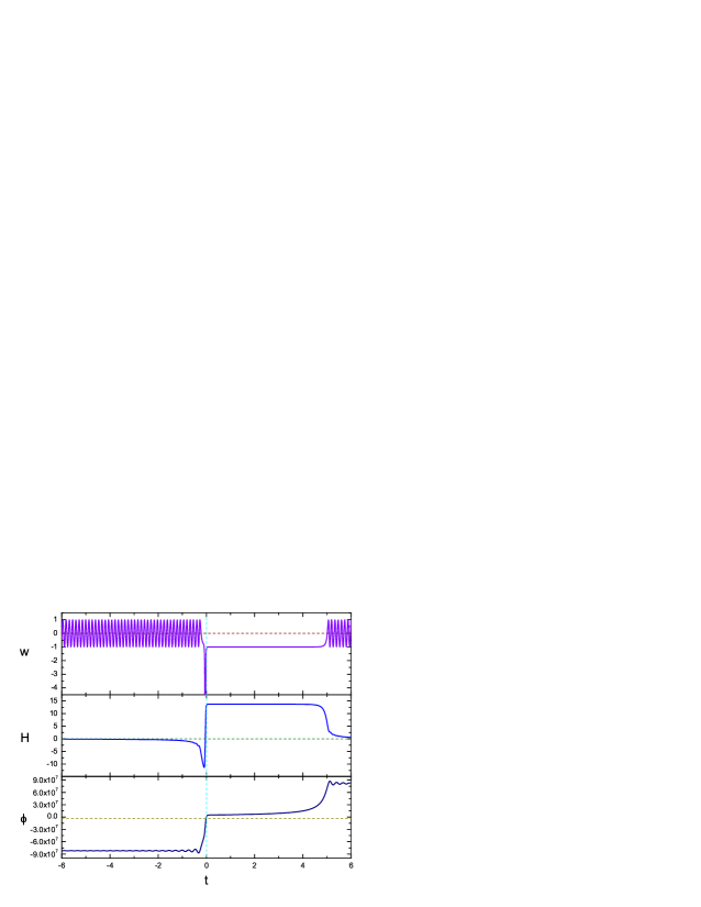
Note that, the asymmetry of the evolution is a significant character since we are able to obtain a scale-invariant spectrum in virtue of this asymmetry. The reason is as follows. Since the evolution of the universe is asymmetric w.r.t. the bounce point, it is possible for the primordial fluctuations keeping inside the horizon when the universe is contracting. And if so, while these perturbations are able to escape to the super-hubble region during the inflationary period, the initial Bunch-Davies condition for them can be basically saved and transferred through the bounce. Therefore, this scenario provides a possible approach to obtaining a scale-invariant spectrum. However, as will be shown in the following, we find that the sub-hubble perturbations still deviate a little from the pure incoming plane wave on the matching surface between the bouncing phase and the expanding phase. This deviation would bring some wiggles on the corresponding scale of the primordial power spectrum, which has been shown in Ref. Cai:2008qb can be detected by the future observations.
Now we take a brief review of the linear curvature perturbation (for details we refer to Ref. Cai:2008qb , and see Ref. MFB for a comprehensive review), then study its evolution in the model of Quintom Bounce and obtain the expression for the primordial power spectrum. Under the longitudinal (conformal-Newtonian) gauge, the metric perturbations are given by
| (3) |
where we introduce the comoving time defined by . We start with the equation of motion of the gravitational potential
| (4) |
where is the comoving hubble parameter and the prime denotes the derivative with respect to the comoving time. This equation can be derived from the basic perturbation equations directly (we refer the complete derivation to Ref. Cai:2007zv ).
As we have pointed out in describing the background evolution, the energy density of the scalar is usually negligible away from the bouncing point and hence we have . Therefore it is a good approximation to neglect the right hand side of Eq. (II) when the universe is far away from the bounce. Moreover, we find that there is the relation in the bouncing phase and so the perturbation of decouples from Eq. (II), which has been checked in Ref. Cai:2007zv . Thus, in the paper we will neglect the r.h.s. of Eq. (II), and just focus on the adiabatic fluctuations which can be determined by a single physical scalar field degree of freedom .
If the evolution of the background is known, all other perturbation variables can be determined from . A frequently used variable is the curvature perturbation in comoving coordinates which is defined as,
| (5) |
and this variable can be calculated from and the background parameters. For example, when the universe is in a nearly de-Sitter like expansion, there is a simple relation with the slow-roll parameter . In usual case this variable is well known to describe the adiabatic perturbations on large scales since it is a conserved quantity on super-hubble scales according to the equation
| (6) |
and its dynamics can be simply and conveniently described by the equation of motion for Mukhanov-Sasaki variable Mukhanov . However, this equation becomes ill-defined both at the bounce point with a vanishing hubble parameter and the cosmological constant boundary . This point has been remarked in Ref. Cai:2007zv ; Brandenberger:2007by ; Xia:2007km . Consequently, we investigate the evolution of the gravitational potential directly in deriving the curvature perturbation, and then moves to after the universe entering the expanding phase.
As introduced in the above, the universe in this model experiences three phases, a contracting one, a bounce, and finally an inflationary one. We can resolve the perturbation equation in each phase respectively. In the detailed calculation, we take the Bunch-Davies vacuum as the initial condition , and then make those solutions smoothly pass through the linking point applying the matching conditionsHwang:1991an (see also Deruelle:1995kd ; Durrer:2002jn ; Copeland:2006tn for a recent study). The detailed derivation has been presented in Ref. Cai:2008qb , and here we give the dominant part of the final gravitational potential directly:
| (7) | |||||
where and represent the comoving hubble parameter at the beginning and the end of the bouncing phase respectively. By comparing the coefficient (7) and the initial form of , obviously the dominant mode of the gravitational potential deviate from the Bunch-Davies initial condition when the inflationary phase takes place. Moreover, we have the approximate relation . So we eventually have the expression of the primordial power spectrum for the curvature perturbation111This result seems similar to an inflation theory with its initial condition as -vacuumDanielsson:2002kx ; Easther:2002xe . However, these two are different in the detailed characteristics of the perturbations and the basic mechanisms for the generation of those perturbations.
| (8) |
From this result, one obviously find that the first term provides a nearly scale-invariant spectrum which is consistent with current cosmological observations. However, the second term shows that there is a wiggle on the spectrum, due to the modified initial condition by the bounce relative to the standard inflation. Apparently, this oscillation term could affect the CMB temperature power spectrum and LSS matter power spectrumCai:2008qb .
III Bispectrum and the non-linear parameter
In this section we investigate the evolution of the nonlinear part of scalar perturbations in our model. As we have discussed in the last section, the universe experiences a nearly exponential expansion after the bounce, and so we can deal with the curvature perturbation of Quintom Bounce as in inflation theory except for the initial condition being modified. Thus, the slow-roll parameters can be defined in our model, with and .
To expand the action to the third order of and drop the terms suppressed by slow-roll parameters and , we have the final cubic action for the curvature perturbation during the inflationary phaseMaldacena:2002vr ,
| (9) |
where
| (10) |
and .
Note that the last term in the third-order action can be absorbed by field redefinitions of . It is taken as
| (11) |
This field redefinitions do not affect any other of the terms in the third-order action, since the term are quadratic in . Moreover, the last term in the third-order action can be cancelled by one extra quadratic part of this field redefinitions which is proportional to the first-order equations of motion exactly.
After deriving out the third-order action, now we are able to get the three point function for our model. It can be computed using the path integral formalism in the interaction picture as follows
| (12) |
where denotes an initial time for the modes deep inside the horizon, and is the third order perturbative lagrangian.
Recall in Eq. (8) we have obtained the linear curvature perturbation which deviates from that in the standard inflation theory by multiplying an extra factor defined as follows,
| (13) |
Considering this factor in the calculations, the leading order
contributions to the three point correlator in our model are
listed in the following,
(a): contribution from . To
make the expression simplified, we define which is just the
curvature spectrum in inflation models and . So we
have the three point correlator from
:
| (14) |
(b): contribution from the field redefinition.
| (15) |
Moreover, since non-Gaussianity measures the deviation of CMB power spectrum from the Gaussian distribution, we can define a non-linear parameter as follows,
| (16) |
So we eventually have to characterize the size of non-Gaussianity,
| (17) |
There are two limiting cases of non-Gaussianity, which are of particular interests for observations. These are equilateral form () and local form (). To the case of equilateral form, is given by
| (18) |
where we have taken the limit . For the local form, which corresponds to that mode exits horizon much earlier than the other two, we have the non-linear parameter
| (19) |
where the limit is taken as . One may notice that, the above results reduce to the single scalar slow-roll inflationary model when . However, since the factor has modified the initial condition of curvature perturbation when the universe enters inflationary stage, it can bring an oscillation signature on the size of non-Gaussianity as well. In order to compare our result with the non-Gaussianity predicted by usual inflation model, we plot of equilateral and local forms in Fig. 2.
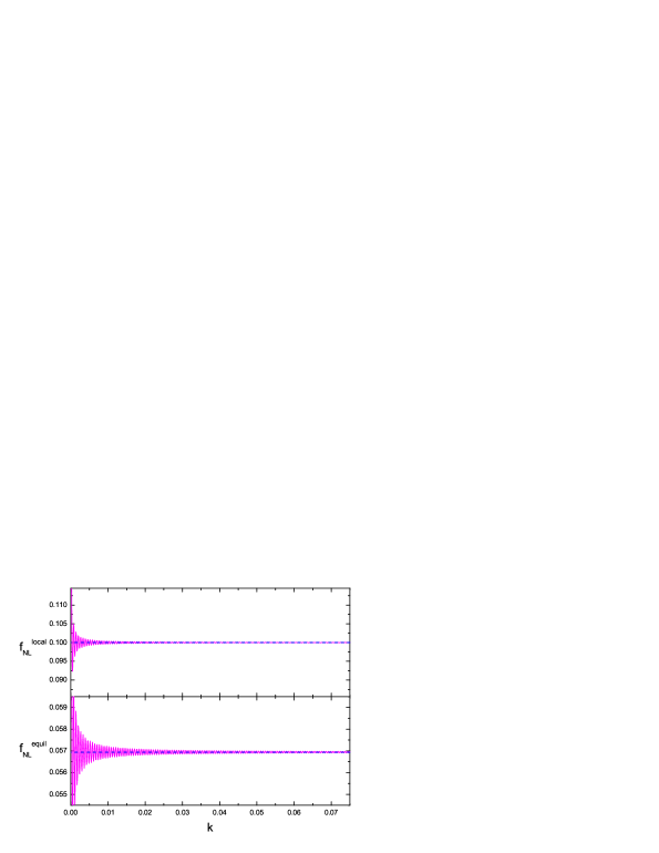
Our results show that the non-Gaussianity in the Quintom Bounce model is still suppressed by the slow-roll parameters. However, there is an oscillation signature on and the maximal value of is bigger than that in single scalar slow-roll inflationary models. The reason for this effect is that the dominant modes of the curvature perturbations have deviated from the Bunch-Davies form when they pass through the bounce and enter the inflationary stage. This is similar to the cases with non-Gaussianity generated from a modified initial condition, for example see Refs. Chen:2006nt ; Holman:2007na ; Chen:2007gd .
IV Gravitational wave background
Now we turn to consider the evolution of gravitational wave background from the tensor part of the primordial metric perturbations. In order to standardize the derivation, we use the same convention as in Ref. Cai:2007xr . To begin with, we give the metric containing the tensor perturbations in the flat FRW background as follows,
| (20) |
where the Latin indexes represent spatial coordinates. Here the tensor perturbation satisfies the following constraints:
| (21) |
Due to these constraints, we only have two degrees of freedom in which correspond to two polarizations of gravitational waves.
By adding the anisotropic part of the stress tensor , we have the equation of motion for tensor perturbations,
| (22) |
The Fourier transformations of the tensor perturbations and anisotropic stress tensor are give by,
| (23) | |||
| (24) |
Note that, what we are usually interested in are the distribution of the spectra of gravitational waves and the corresponding spectral index. Based on the above formalism, the tensor power spectrum can be written as,
| (25) |
and the definition of tensor spectral index is given by
| (26) |
The GWB we observed today is characterized by the energy spectrum,
| (27) |
where is the energy density of gravitational waves, and the parameter is the critical density of the universe. In respect that the GWB we observed has already reentered the horizon, the modes should oscillate in the form of a sinusoidal function. Consequently, we can make use of the Friedmann equation and then deduce the relation between the power spectrum and the energy spectrum as follows,
| (28) |
which will be used in the following calculations.
IV.1 Tensor perturbations
Now we follow one Fourier mode of the tensor perturbations, labelled by its comoving wave number , and find that there are two paths which are different in the times of crossing the hubble radius. The evolution of tensor perturbations is sketched in Fig. 3. Initially all the perturbations stay inside the hubble radius in the far past. Since the hubble radius shrinks in the contracting phase, those modes with small comoving wave number exit the hubble radius while the large scales still keep inside. When the bounce takes place, all the perturbations will keep inside the hubble radius because at that moment the hubble radius diverges. After that the bounce is followed by a slow-roll expanding phase, so these Fourier modes will escape out if the efolds for the post-bounce inflationary period is large enough. After that, these modes will reenter the hubble radius at late times after the slow-roll expanding phase has finished.
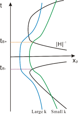
Therefore, we can classify the tensor perturbations with different comoving wave numbers to two categories, as the two lines sketched in Fig. 3. The blue line denotes a mode with a scale which is large enough to keep it inside the hubble radius through the contracting phase and the bounce, and then escape outside during the post-bounce inflationary period; the green line consists of a mode with small so that it exits the hubble radius in the contracting phase, then is pushed inside during the bounce and soon is pulled outside before the slow-roll expanding phase happens.
Due to the symmetry of , we can express the two polarizations as one function . Neglecting the anisotropic stress tensor in the very early universe, we obtain the equation of motion for :
| (29) |
Following the background evolution of the universe, we obtain three solutions of gravitational waves similar to what we did with scalar perturbations. For the universe which is contracting with its EoS oscillating around , we have
| (30) | |||||
where . Here and are the -th Hankel function of the first kind and second kind respectively. Besides, the parameters and can be determined by the initial condition for gravitational waves, which is usually taken as Bunch-Davies vacuum . So we have and . Therefore, the asymptotic forms of the solution to the tensor perturbation in the contracting phase is
| (34) |
When the universe undergoes the bouncing phase, we have the approximate relation that . To solve Eq. (29), we have
| (38) |
where we define . Since the hubble parameter approaches zero when the universe is bouncing from a contraction to an expanding phase, all the modes of the perturbations would return to the sub-hubble region. However, from the above solution we interestingly find that, and are comparable.
After the bounce, the slow-roll expanding phase takes place which drives the universe to inflate like a de-Sitter spacetime. In this case, the solution to the gravitational waves is given by
| (39) | |||||
where . This solution has an asymptotic form,
| (40) |
after the modes exit the horizon.
Having obtained the solutions of the tensor perturbations in different phases, now we need to match these solutions and determine the coefficients , , and respectively. This procedure is much similar to the matching process of scalar perturbations as done in the previous section. For a non-singular bounce scenario such as the Quintom Bounce model, the continuity of background evolution implies that both and are able to pass through the bounce smoothly. So we match and in (34) and (38) on the surface , and those in (38) and (39) on the surface . With these matching conditions, we can determine all the coefficients and finally get .
However, as what we have analyzed at the beginning of this section, there are two paths for the tensor perturbations to evolve from a contracting phase to an expanding phase. So there are two possible results for . For the first case, the comoving wave number is large enough so that the tensor perturbations have never escape outside the hubble radius, thus we have
| (41) |
where , and . For the second case where the modes of gravitational waves are in small region, the expression is given by
| (42) |
Based on the above analysis, now we are able to derive the primordial power spectrum of gravitational waves. From the definition of Eq. (25), the primordial power spectrum is given by
| (43) |
From Eqs. (41) and (42), we can read that the spectrum are scale-invariant both at the large and small region, but oscillate when is near to a critical value . To illustrate the above analysis clearly, we do the numerical calculation and plot the results of primordial tensor power spectrum and the corresponding spectral index in Fig. 4.
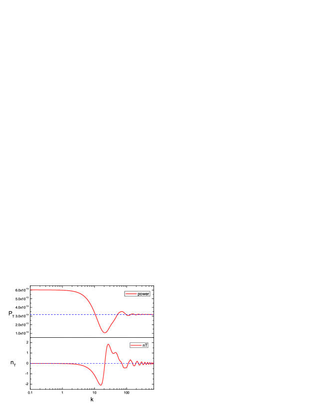
One can see that in Fig. 4, when the value of is large enough, the red solid lines converge at the blue dash lines with an oscillation. The amplitude of the oscillation gets the largest value when approaches the neighborhood of the critical value , and soon drop down to a minimal value when gets smaller. This damping effect is caused by the modified dispersion relation of the tensor perturbations when they pass through the bouncing phase222A similar scenario of the primordial gravitational waves has been considered in Ref. Cai:2007xr , where the authors have considered the damping effects from the spacetime noncommutativity. . However, when the comoving wave number gets even smaller, the power spectrum is able to climb up and finally reaches a certain value with its spectral index returning to zero again.
IV.2 Energy Spectrum of Today’s GWB
In the above section we discussed the behavior of tensor perturbations exhibited in primordial power spectrum and the spectral index. However, we are more interested in how to recognize these perturbations in the GWB nowadays. Since the primordial gravitational waves are distributed in every frequency, once the effective co-moving wave number is less than , the corresponding mode of gravitational waves would escape the horizon and be frozen until it reenters the horizon. The relation between the time when tensor perturbations exit the horizon and the time when they return is . Therefore, we have the conclusion that, the earlier the perturbations escape the horizon, the later they re-enter it. Moreover, once the effective co-moving wave number is larger than , the perturbations begin to oscillate like the plane wave, as shown in Fig. 3.
To relate the power spectrum observed today to the primordial one, one can define a transfer function , given by Refs. Boyle:2005se ; Cai:2007xr :
| (44) |
where is determined by the EoS of the universe, is the redshift at the moment and is the redshift when the mode of gravitational wave reenters the horizon. Here the factor comes from the damping effect of freely streaming neutrinos Weinberg:2003ur . Moreover, the factor describes the redshift-suppressing effect on the primordial gravitational waves. The rest factor shows that, when the gravitational waves reenter the horizon, there is a “wall” lying on the horizon which affects the tensor spectrum.
Considering today our universe is dominated by dark energy of which the EoS is , we are able to obtain today’s transfer function. Then we can get today’s tensor power spectrum
| (45) |
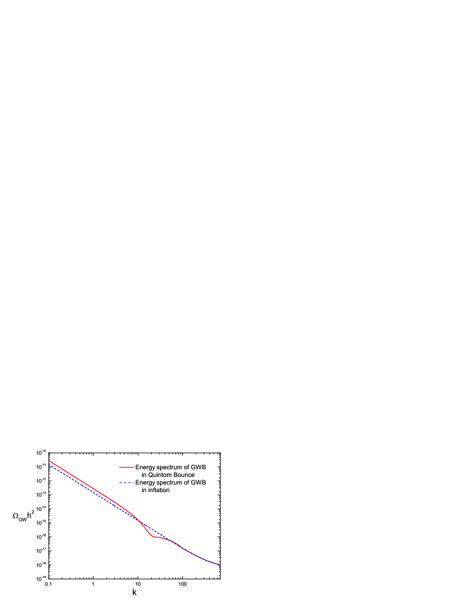
where represents the hubble parameter in the inflationary stage. Eventually, the present energy spectrum of GWB is given by .
In Fig. 5 we plot the numerical results of the energy spectrum in our model. One can see that, when the frequency of GWB is large enough, the tensor energy spectrum of our model would agree with the prediction of the single scalar inflationary model. However, when the frequency becomes smaller, the physics of a bounce begins to affect the behavior of the GWB. Moreover, there is an interesting sunken area in the middle band. This sunken signal is resulted from the modified dispersion relation of the tensor perturbations when they pass through the bouncing phase.
V Discussion and Conclusions
Bouncing cosmology, due to the avoidance of the initial singularity, has attracted a lot of interests in the literature Peter ; Veneziano ; Wands ; Piao:2004me ; Senatore ; Buchbinder:2007ad ; ArmendarizPicon:2003qk (and see Ref. Novello:2008ra for a recent review). However, since it happens in extremely high energy regime, we hardly observe a bounce by experiments directly. So it is a debate whether a bounce has taken place or not. To find the evidences of a bounce, we need to know what can a bounce leave for observations. This question is still discussed drastically in the literature, and one potential clue is to study the primordial gravitational fluctuations. In the context of the Pre-Big-Bang scenario and in the cyclic/Ekpyrotic cosmology, the primordial curvature perturbation strongly depends on the physics at the epoch of thermalization, and thus an uncertainty of a thermalized surface is involved BGGMV ; Lyth ; Hwang2 ; Fabio ; Tolley:2003nx . In the frame of loop quantum cosmology, it is argued that fluctuations before and after the bounce are largely independent Bojowald:2007zza (yet see Ref. Corichi:2007am for some criticisms). We in this paper have studied the perturbation theory of a Quintom Bounce model detailedly and show that there are some imprints of the bounce on CMB observations at large scales. In the main content we have analyzed both the linear and non-linear evolutions of scalar modes, and the tensor perturbations are also considered.
The model we considered is constructed by a double field Quintom model with a Coleman-Weinberg potential. We firstly have reviewed the background dynamics of this model, and obtained a scale-invariant scalar spectrum in virtue of an asymmetry of the background evolution around the bounce point. A similar but more phenomenological scenario has been studied in Refs. Piao:2003zm as a possible solution to the suppressed low multi-poles of the CMB anisotropies. Moreover, since the gravitational perturbations in sub-hubble region would change their propagations when pass through the surface between the contracting phase and the bounce, there would be an oscillation signature generated both on the linear scalar modes and non-linear ones. We have also calculated the non-Gaussianity and shown that the maximal value of non-linear parameter predicted by our model is mildly bigger than the usual one in single scalar slow-roll inflation, but the central value is still suppressed by the slow-roll parameters. So we expect that a large non-Gaussianity might be generated by other mechanismsLi:2008fm in the frame of Quintom Bounce.
We in the last part of this paper focus on the behavior of the gravitational waves in Quintom Bounce. Due to the effects of a bounce, the solution of the tensor perturbation is quite different from the usual one. In our analysis, we find that the physics of a bounce would affect the evolution of primordial tensor perturbations at large scales of the universe, which corresponds to the physics in very early time. The behavior of the energy spectrum of the GWB in our model is similar to that in the single scalar inflationary model in high-frequency regime. However, for low-frequency regime the difference becomes larger. Moreover, there is a sunken area in the middle band which links high-frequency regime and low-frequency regime. If these signals would be detected, these might act as a smoking gun to the bouncing cosmology.
Acknowledgements.
We thank Hong Li, Mingzhe Li, Jie Liu, Yun-Song Piao, Taotao Qiu and Jun-Qing Xia for helpful discussions. This work is supported in part by National Natural Science Foundation of China under Grant Nos. 10533010 and 10675136 and by the Chinese Academy of Science under Grant No. KJCX3-SYW-N2.References
- (1) A. H. Guth, Phys. Rev. D 23, 347 (1981); A. Albrecht and P. J. Steinhardt, Phys. Rev. Lett. 48, 1220 (1982); A. D. Linde, Phys. Lett. B 108, 389 (1982).
- (2) A. A. Starobinsky, Phys. Lett. B 91, 99 (1980); K. Sato, Mon. Not. Roy. Astron. Soc. 195, 467 (1981).
- (3) A. Borde and A. Vilenkin, Phys. Rev. Lett. 72, 3305 (1994).
- (4) G. Veneziano, Phys. Lett. B 265, 287 (1991); M. Gasperini and G. Veneziano, Astropart. Phys. 1, 317 (1993); M. Gasperini and G. Veneziano, Phys. Rept. 373, 1 (2003).
- (5) J. Khoury, B. A. Ovrut, P. J. Steinhardt and N. Turok, Phys. Rev. D 64, 123522 (2001); J. Khoury, B. A. Ovrut, N. Seiberg, P. J. Steinhardt and N. Turok, Phys. Rev. D 65, 086007 (2002); P. J. Steinhardt and N. Turok, Phys. Rev. D 65, 126003 (2002).
- (6) M. Bojowald, Phys. Rev. Lett. 86, 5227 (2001).
- (7) R. Brustein and R. Madden, Phys. Rev. D 57, 712 (1998).
- (8) T. Biswas, A. Mazumdar and W. Siegel, JCAP 0603, 009 (2006); T. Biswas, R. Brandenberger, A. Mazumdar and W. Siegel, JCAP 0712, 011 (2007).
- (9) M. Novello and S. E. P. Bergliaffa, Phys. Rept. 463, 127 (2008).
- (10) Y. F. Cai, T. Qiu, Y. S. Piao, M. Li and X. M. Zhang, JHEP 0710, 071 (2007).
- (11) B. Feng, X. L. Wang and X. M. Zhang, Phys. Lett. B607, 35 (2005).
- (12) Y. F. Cai, T. Qiu, R. Brandenberger, Y. S. Piao and X. Zhang, JCAP 0803, 013 (2008).
- (13) L. R. Abramo and P. Peter, JCAP 0709, 001 (2007).
- (14) R. Brandenberger, H. Firouzjahi and O. Saremi, JCAP 0711, 028 (2007).
- (15) R. Brustein, M. Gasperini, M. Giovannini, V. F. Mukhanov and G. Veneziano, Phys. Rev. D 51, 6744 (1995).
- (16) D. H. Lyth, Phys. Lett. B 524, 1 (2002).
- (17) J. C. Hwang, Phys. Rev. D 65, 063514 (2002).
- (18) F. Finelli and R. Brandenberger, Phys. Rev. D 65, 103522 (2002).
- (19) Y. F. Cai, T. T. Qiu, J. Q. Xia, H. Li and X. M. Zhang, arXiv:0808.0819 [astro-ph].
- (20) N. Bartolo, E. Komatsu, S. Matarrese and A. Riotto, Phys. Rept. 402, 103 (2004).
- (21) J. M. Maldacena, JHEP 0305, 013 (2003).
- (22) V. Acquaviva, N. Bartolo, S. Matarrese and A. Riotto, Nucl. Phys. B 667, 119 (2003).
- (23) K. Koyama, S. Mizuno, F. Vernizzi and D. Wands, JCAP 0711, 024 (2007).
- (24) E. I. Buchbinder, J. Khoury and B. A. Ovrut, Phys. Rev. Lett. 100, 171302 (2008).
- (25) J. L. Lehners and P. J. Steinhardt, Phys. Rev. D 77, 063533 (2008); J. L. Lehners and P. J. Steinhardt, Phys. Rev. D 78, 023506 (2008).
- (26) Y. S. Piao, Nucl. Phys. B 803, 194 (2008); Y. S. Piao, arXiv:0807.3813 [gr-qc].
- (27) A. P. S. Yadav and B. D. Wandelt, Phys. Rev. Lett. 100, 181301 (2008).
- (28) E. Komatsu et al. [WMAP Collaboration], arXiv:0803.0547 [astro-ph].
- (29) PLANCK Collaboration, arXiv:astro-ph/0604069.
- (30) http://universe.nasa.gov/program/vision/bbo.html
- (31) B. Abbott et al. [LIGO Scientific Collaboration], Phys. Rev. Lett. 94, 181103 (2005).
- (32) L. Verde, H. Peiris and R. Jimenez, JCAP 0601, 019 (2006).
- (33) T. L. Smith, M. Kamionkowski and A. Cooray, Phys. Rev. D 73, 023504 (2006).
- (34) L. A. Boyle, P. J. Steinhardt and N. Turok, Phys. Rev. Lett. 96, 111301 (2006).
- (35) R. Weiss et al., Task Force On Cosmic Microwave Research, (www.science.doe.gov/hep/TFCRreport.pdf).
- (36) L. P. Grishchuk, Sov. Phys. JETP 40, 409 (1975) [Zh. Eksp. Teor. Fiz. 67, 825 (1974)].
- (37) B. Allen, Phys. Rev. D 37, 2078 (1988).
- (38) A. A. Starobinsky, JETP Lett. 30, 682 (1979) [Pisma Zh. Eksp. Teor. Fiz. 30, 719 (1979)]; V. A. Rubakov, M. V. Sazhin and A. V. Veryaskin, Phys. Lett. B 115, 189 (1982); R. Fabbri and M. d. Pollock, Phys. Lett. B 125, 445 (1983); L. F. Abbott and M. B. Wise, Nucl. Phys. B 244, 541 (1984).
- (39) E. D. Stewart and D. H. Lyth, Phys. Lett. B 302, 171 (1993).
- (40) L. A. Boyle, P. J. Steinhardt and N. Turok, Phys. Rev. D 69, 127302 (2004).
- (41) S. R. Coleman and E. Weinberg, Phys. Rev. D 7, 1888 (1973).
- (42) R. H. Brandenberger, arXiv:hep-ph/9910410.
- (43) A. D. Linde, arXiv:hep-th/0503203.
- (44) V. F. Mukhanov, H. A. Feldman and R. H. Brandenberger, Phys. Rept. 215, 203 (1992).
- (45) V. F. Mukhanov, Sov. Phys. JETP 67, 1297 (1988) [Zh. Eksp. Teor. Fiz. 94N7, 1 (1988)]; M. Sasaki, Prog. Theor. Phys. 76, 1036 (1986).
- (46) J. Q. Xia, Y. F. Cai, T. T. Qiu, G. B. Zhao and X. Zhang, arXiv:astro-ph/0703202; Y. F. Cai, H. Li, Y. S. Piao and X. M. Zhang, Phys. Lett. B 646, 141 (2007); Y. F. Cai, M. Z. Li, J. X. Lu, Y. S. Piao, T. T. Qiu and X. M. Zhang, Phys. Lett. B 651, 1 (2007).
- (47) J. C. Hwang and E. T. Vishniac, Astrophys. J. 382, 363 (1991).
- (48) N. Deruelle and V. F. Mukhanov, Phys. Rev. D 52, 5549 (1995).
- (49) R. Durrer and F. Vernizzi, Phys. Rev. D 66, 083503 (2002).
- (50) E. J. Copeland and D. Wands, JCAP 0706, 014 (2007).
- (51) U. H. Danielsson, Phys. Rev. D 66, 023511 (2002).
- (52) R. Easther, B. R. Greene, W. H. Kinney and G. Shiu, Phys. Rev. D 66, 023518 (2002).
- (53) X. Chen, M. X. Huang, S. Kachru and G. Shiu, JCAP 0701, 002 (2007).
- (54) R. Holman and A. J. Tolley, JCAP 0805, 001 (2008).
- (55) B. Chen, Y. Wang and W. Xue, JCAP 0805, 014 (2008); W. Xue and B. Chen, arXiv:0806.4109 [hep-th].
- (56) Y. F. Cai and Y. S. Piao, Phys. Lett. B 657, 1 (2007).
- (57) L. A. Boyle and P. J. Steinhardt, Phys. Rev. D 77, 063504 (2008).
- (58) S. Weinberg, Phys. Rev. D 69, 023503 (2004).
- (59) P. Peter and N. Pinto-Neto, Phys. Rev. D 66, 063509 (2002).
- (60) M. Gasperini, M. Giovannini and G. Veneziano, Phys. Lett. B 569, 113 (2003).
- (61) L. E. Allen and D. Wands, Phys. Rev. D 70, 063515 (2004).
- (62) Y. S. Piao, Phys. Rev. D 70, 101302 (2004); Y. S. Piao and Y. Z. Zhang, Nucl. Phys. B 725, 265 (2005).
- (63) P. Creminelli and L. Senatore, JCAP 0711, 010 (2007).
- (64) E. I. Buchbinder, J. Khoury and B. A. Ovrut, Phys. Rev. D 76, 123503 (2007); E. I. Buchbinder, J. Khoury and B. A. Ovrut, JHEP 0711, 076 (2007).
- (65) C. Armendariz-Picon and P. B. Greene, Gen. Rel. Grav. 35, 1637 (2003); Y. F. Cai and J. Wang, Class. Quant. Grav. 25, 165014 (2008); S. Alexander and T. Biswas, arXiv:0807.4468 [hep-th]; M. R. Setare, J. Sadeghi and A. Banijamali, arXiv:0807.0077 [hep-th].
- (66) A. J. Tolley, N. Turok and P. J. Steinhardt, Phys. Rev. D 69, 106005 (2004).
- (67) M. Bojowald, Nature Phys. 3N8 (2007) 523.
- (68) A. Corichi and P. Singh, Phys. Rev. Lett. 100, 161302 (2008).
- (69) Y. S. Piao, B. Feng and X. M. Zhang, Phys. Rev. D 69, 103520 (2004); Y. S. Piao, S. Tsujikawa and X. M. Zhang, Class. Quant. Grav. 21, 4455 (2004); J. Mielczarek, arXiv:0807.0712 [gr-qc].
- (70) S. Li, Y. F. Cai and Y. S. Piao, arXiv:0806.2363 [hep-ph].